International Doctorate School in Information and Communication Technologies
DISI - University of Trento
Human Activity Analytics
Based on Mobility and Social Media Data
Pavlos Paraskevopoulos
Advisor:
Prof. Themis Palpanas
Universit´e Paris-Descartes, France Universit`a degli Studi di Trento, Italy
Thesis Committee:
Prof. Barbara Catania, Universit`a degli Studi di Genova, Italy Prof. Alessandro Moschiti, Universit`a degli Studi di Trento, Italy Prof. Myra Spiliopoulou, Universit¨at Magdeburg, Germany Prof. Athena Vakali, Aristotle University, Greece
The development of social networks such as Twitter, Facebook and Google+ allow users to share their beliefs, feelings, or observations with their circles of friends. Based on these data, a range of applications and techniques has been developed, targeting to provide a better quality of life to the users. Nevertheless, the quality of results of the geolocation-aware applications is significantly restricted due to the tiny percentage of the social media data that is geotagged ( 2% for Twitter). Hence, increasing this percentage is an important and challenging problem. Moreover, information extracted from social media data can be complemented by the analysis of mobile phone usage data, in order to provide further insights on human activity patterns.
In this thesis, we present a novel method for analyzing and geolocalizing non-geotagged Twitter posts. The proposed method is the first to do so at the fine-grain of city neighbor-hoods, while being both effective and time efficient. Our method is based on the extraction of representative keywords for each candidate location,as well as the analysis of the tweet volume time series. We also describe a system built on top of our method, which geolocal-izes tweets and allows users to visually examine the results and their evolution over time. Our system allows the user to get a better idea of how the activity of a particular location changes, which the most important keywords are, as well as to geolocalize individual tweets of interest. Moreover, we study the activity and mobility characteristics of the users that post geotagged tweets and compared the mobility of users who attended the event with a random set of users. Interestingly, the results of this analysis indicate that a very small number of users (i.e., less than 35 users in this study) is able to represent the mobility patterns present in the entire dataset.
Finally, we study the call activity and mobility patterns, clustering the observed behav-iors that exhibited similar characteristics, and characterizing the anomalous behavbehav-iors. We analyzed a Call Detail Record (CDR) dataset, containing (aggregated) information on the calls among mobile phones. Employing density-based algorithms and statistical anal-ysis, we developed a framework that identifies abnormal locations, as well abnormal time intervals. The results of this work can be used for early identification of exceptional situ-ations, monitoring the effects of important events in urban and transportation planning, and others.
Pavlos Paraskevopoulos
1 Introduction 1
1.1 Geolocalized Posts on Social Media . . . 2
1.2 Characterizing User Behavior Patterns Based on The Calling Activity . . . 5
1.3 Summary of Contributions . . . 6
1.3.1 Publications Produced . . . 7
2 Related Work 9 2.1 Geolocalisation of Social Media Posts . . . 9
2.2 Analyzing Mobile Phone Usage Data . . . 12
3 Fine-Grained Geolocalization of Non-Geotagged Tweets 15 3.1 Introduction . . . 15
3.2 Problem Formulation . . . 16
3.3 Proposed Approach . . . 16
3.3.1 Grouping the Posts and Extracting Important Keywords . . . 17
3.3.2 Similarity Calculation and Best Match Extraction . . . 18
3.3.3 Similarity Based on Correlation of Activity Time Series . . . 19
3.3.4 Filtering out Candidate Locations Based on Linear Regression . . . 20
3.3.5 Sliding Windows . . . 21
3.3.6 Dynamic Threshold Extraction . . . 23
3.3.7 Logistic Regression . . . 24
3.4 Experimental Evaluation . . . 24
3.4.1 Evaluating the basic Algorithms . . . 24
3.4.2 Evaluating the Algorithms with Linear Regression . . . 32
3.4.3 Evaluation of SDpL and MDpL . . . 48
3.5 Summary . . . 50
4.2 System Functionality . . . 59
4.3 Summary . . . 60
5 What do Geotagged Tweets Reveal about the Users? 65 5.1 Introduction . . . 65
5.2 Problem Description . . . 65
5.3 Proposed Approach . . . 66
5.3.1 Setting the temporal and spatial parameters . . . 66
5.3.2 Get the Event and CGL users . . . 66
5.3.3 Cleaning the Dataset . . . 67
5.3.4 Activity and Movement Comparison . . . 67
5.4 Experimental Evaluation . . . 68
5.4.1 Datasets . . . 68
5.4.2 Top and Random Users from Italy . . . 74
5.4.3 Cumulative Distribution Function and Movement . . . 88
5.5 Summary . . . 93
6 Identifying Abnormal Spatio-Temporal Patterns in Mobile Phone Usage Data 95 6.1 Introduction . . . 95
6.2 Problem description . . . 95
6.3 Methodology . . . 96
6.3.1 Preprocessing of Datasets . . . 96
6.3.2 Analysis of Anomalous Behavior . . . 98
6.4 Experimental Evaluation . . . 101
6.4.1 Description of Datasets . . . 101
6.4.2 Anomalous behaviors . . . 103
6.5 Summary . . . 105
7 Conclusions and Future Work 107 7.1 Conclusions . . . 107
7.2 Future Work . . . 108
7.2.1 Enhancing the Geolocalization Techniques . . . 108
7.2.2 Extending the Applicability of the proposed Techniques . . . 109
7.2.3 Predict Mobility Based on Social Media Posts . . . 109 7.2.4 Predicting Human Activity Based on Social Media and Forum Posts 110
6.1 List of important regional and national events in Ivory Coast, for the time period between December 2011 and April 2012. . . 102
1.1 Example of Tweet that includes Text Content, an Image, the Username,
and Timestamp . . . 2
1.2 Data generated from different neighborhoods (i.e., squares with side 1000 meters) in Milan (Italy), for time intervals of 4 hours, between June 20 and July 23, 2014. . . 4
3.1 Accuracy for city level when using TG, TG-C, TG-TI, and TG-TI-C (@0-Step). . . 26
3.2 Trade-off Between Execution Time and Accuracy for Neighbourhood Level (@Top1 and @0-Step). . . 28
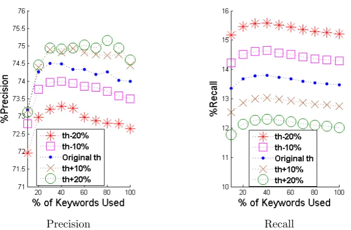
3.3 Precision and recall on Neighbourhood Level for TG when using dynamic thresholds (Th) (@Top1 and @0-Step). . . 29
3.4 Precision and recall on Neighbourhood Level for TG-TI-C when using dy-namic thresholds (Th) (@Top1 and @0-Step). . . 29
3.5 F1 measure for Neighbourhood Level without and with threshold (Th) (@Top1 and @0-Step). . . 30
3.6 Accuracy for Neighbourhood Level for TG, TG-C, TG-TI, and TG-TI-C (@0-Step). . . 31
3.7 Accuracy for Neighbourhood Level (@Top1). . . 31
3.8 TG-CLR for Different LR Parameters (@Top1 and @0-Step). . . 34
3.9 TG-TI-CLR for Different LR Parameters (@Top1 and @0-Step). . . 34
3.10 F1 for TG-CLR and TG-TI-CLR for Different LR Parameters (@Top1 and @0-Step). . . 35
3.11 Trade-off Between Precision and Recall for Neighbourhood Level (Milan, @Top1 and @0-Step). . . 36
3.12 Precision and Recall for the City of Rome (@Top1 and @0-Step). . . 37
3.13 Precision and Recall for the City of Berlin (@Top1 and @0-Step). . . 37
3.14 Precision and Recall for the City of Amsterdam (@Top1 and @0-Step). . . 38
3.16 Precision and Recall on Neighbourhood Level for TG-TI when using
dy-namic thresholds (Th) (@Top1 and @0-Step). . . 39
3.17 Precision and Recall on Neighbourhood Level for TG-TI-CLR1 when using dynamic thresholds (Th) (@Top1 and @0-Step). . . 40
3.18 F1 measure for Neighbourhood Level with threshold (Th) (@Top1 and @0-Step). . . 41
3.19 Precision and Recall for TG-TI (@0-Step). . . 42
3.20 Precision and Recall for TG-TI-CLR1 (@0-Step). . . 42
3.21 F1 Score for TG-TI and TG-TI-CLR1 (@0-Step). . . 43
3.22 Precision for Neighbourhood Level (@Top1). . . 44
3.23 Recall for Neighbourhood Level (@Top1). . . 45
3.24 Precision and Recall for TG-TI-CLR1 for varying similarity threshold, TopK, and @Step. . . 46
3.25 Precision and Recall Comparison for the City of Rome (grids 20x20 and 30x30, @Top1 and @0-Step). . . 46
3.26 (Top) Trade-off Between Precision and Recall for 7 CGLs (Rome, Milan, Venice, Florence, Naples, Bologna, Turin, @Top1). (Bottom) F1 for 1 and 7 CGLs (@Top1). . . 51
3.27 Precision, Recall and F1 Comparison for 7 CGRs (@Top1) . . . 52
3.28 (Top) Vatican (1.3km-side square / @Top1). (Bottom) San Siro (0.8km-side square / @Top1). . . 53
3.29 Trade-off Between Accuracy and the Number of Candidate Locations (MDpL and SDpL ) . . . 54
3.30 Precision and Recall of MDpL . . . 54
3.31 Precision and Recall of SDpL . . . 55
3.32 F1 of MDpL and SDpL . . . 55
4.1 TweeLoc Architecture . . . 58
4.2 Country and City Activity Heatmaps . . . 61
4.3 FGL Activity and Differential Heatmaps . . . 62
4.4 FGL and Activity Tweet Details . . . 63
5.1 Concert1, window of 24 hours (67 users) . . . 75
5.2 Concert1, window of 48 hours (144 users) . . . 76
5.3 Vatican Visitors, window of 24 hours (48 users) . . . 77
5.4 Vatican Visitors, window of 48 hours (91 users) . . . 78
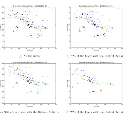
5.7 Parliament Visitors Manually Filtered, window of 24 hours (24 users) . . . 81
5.8 Parliament Visitors Manually Filtered, window of 48 hours (46 users) . . . 82
5.9 Concert1 and Rome Visitors (Random 16 VS Top 16) . . . 84
5.10 Concert1 and Rome Visitors (Random 33 VS Top 33) . . . 85
5.11 Concert1 and Rome Visitors (Random 50 VS Top 50) . . . 86
5.12 Concert1 and Rome Visitors (Random 67 VS Top 67) . . . 87
5.13 Concert1 and Italy Visitors (Random 16 VS Top 16) . . . 89
5.14 Concert1 and Italy Visitors (Random 33 VS Top 33) . . . 90
5.15 Concert1 and Italy Visitors (Random 50 VS Top 50) . . . 91
5.16 Concert1 and Italy Visitors (Random 67 VS Top 67) . . . 92
5.17 CDF: Comparison of Number of Tweets . . . 93
6.1 Daily plot for dpc normalized by day. . . 99
6.2 Cell-Towers Positive Outliers for 9-10 of February 2012 . . . 104
6.3 Cell-Towers Negative Outliers for 3 of February 2012 . . . 104
6.4 Number of calls for each day (normalized by day) . . . 105
6.5 Weights For The Correlation of The Two Types of Normalized Values For The Duration (for each cell-tower) . . . 106
Introduction
It’s the time you spent on your rose that makes your rose so
important...People have forgotten this truth, but you mustn’t forget it. You become responsible forever for what you’ve tamed.
You’re responsible for your rose.
Antoine de Saint-Exupery, The Little Prince
Events that happen around us affect our lives to different degrees. The effects of an event on a community vary depending on the type of the event and its dynamics. For example, traffic jams affect the way we move, football matches and concerts may affect the normal pace of life in the area of the venue for a short period of time, while earthquakes and diseases are unpredicted events, which could cause significant problems that have to be addressed fast. Many entities, public and private, are interested in analyzing the effects of such events, in order to better understand and react to them, and lead to a better quality of life. For example, the identification of lack of clean water at a place would lead the water providers to take special care for resolving the problem. Even though this would be a manual, labour-intensive, and time-consuming process in the past (e.g., consider the 1854 cholera outbreak in London [36]), this is no longer the case.
con-Figure 1.1: Example of Tweet that includes Text Content,
an Image, the Username, and Timestamp
taining the approximate location of the user, which is recorded by the mobile network providers.
1.1
Geolocalized Posts on Social Media
Although all the data generated on social networks are important, the data generated from mobile devices are more valuable due to the fact that they can describe the events in real time, also providing the exact location.
Twitter1 is one of the most famous social networks, counting more than 313M monthly active users, 82% of which are on mobile devices. The posts generated from Twitter are called “tweets” and they contain raw text, hashtags and the time they were posted, while the user has the option to include the location. Also, the sharing of photos and links is possible, while other users can retweet or favorite the post. An example of a tweet is presented in Figure 1.1 which is a tweet posted by Podolski, a player of the German national team, at the matchday of the final of the World Cup 2014.
1
Posts like the one presented in Figure1.1 contain important information that can be used for the better and more detailed understanding of social activities. To that effect, several studies [70], including applications [8; 9; 20; 27; 45; 62; 71; 73; 79] and techniques [30; 43; 55; 69; 72; 74] have been developed that analyze datasets created through the use of social networks, in order to provide benefits to end users, businesses, civil authorities and scientists alike [57].
Several of these applications, depend on the knowledge of the user location at the time of the posting. For example, this knowledge is necessary for applications that target to characterize an urban landscape, or to optimize urban planning [27], to identify and report natural disasters, such as earthquakes [20; 62], and to monitor and track mobility and traffic [9]. Such applications, which represent an increasingly wide range of domains, are restricted to the use of geotagged data2, that is, posts in social networks containing the geographic coordinates of the user at the time of posting.
Evidently, the availability of geotagged data, determines not only the possibility to use such applications, but also their quality-performance characteristics: the more geotagged data posts are available, the better the quality of the results will be (more accurately: the higher the probability for being able to produce better quality results). Nevertheless, the availability of geotagged data is rather limited. In Twitter, which is the focus of our study, the number of geotagged tweets is a mere 1.5-3% of the total number of tweets [31; 39; 49]. As a result, the amount of useful data for these applications to analyze is small, which in turn limits the utility of the applications. Even if we considered this subset of geotagged tweets as representative, “there is a tendency for geotaggers to be slightly older than non-geotaggers” [65], which may lead to non-representative, or skewed results.
In this thesis, we address this problem by describing a method for geolocalising tweets that are non-geotagged. Even though previous works have recognized the importance and have studied this problem [16; 37] (for a comprehensive discussion of this problem refer to [31]), their goal was to produce a coarse-grained estimate of the location of a set of non-geotagged tweets (e.g., those originating from a single user). The algorithms they propose operate at the level of postal zipcodes, cities, and geographical areas larger than cities. In contrast, we study this problem at a much finer granularity, providing location estimates for individual tweets first at the level of cities, and then at the level of city neighborhoods. More precisely, we focused on the identification of the location, where the location belonged to a set of candidate locations. This solution exploits the similarities in the content between an individual tweet and a set of geotagged tweets, as well as their time-evolution characteristics. We first determine the city, and then the neighborhood in the city, by building content-based models and analyzing the volume of posts over time,
2
Number of Tweets Appearances of Words
Figure 1.2: Data generated from different neighborhoods (i.e., squares with side 1000 meters)
in Milan (Italy), for time intervals of 4 hours, between June 20 and July 23, 2014.
independently for each one of these two levels. Using this set up, we are able to effectively predict the location of a post from the Twitter stream, when the only input we have is the actual content of the post and its timestamp.
In addition, we study the specific problem of geolocalising tweets deriving from tar-geted locations of interest, that is, neighborhoods of a particular cultural, social, or touris-tic importance (e.g., the Vatouris-tican in Rome). Our experiments show that we can reuse our technique for this case, as well, by adjusting its operation to this context, where a small number of popular keywords mentioned in the posts characterize the location.
Figure 1.2(a) depicts the number of tweets posted from the neighborhood in which the “SanSiroStadium” is located, and from a neighborhood located in the center of the Milan (Italy), while Figure 1.2(b) shows the number of appearances of the keywords concert(in English and Italian) and stadium/siro in these neighborhoods. As these graphs show, the “San Siro” geolocation exhibits an unusually high activity during the time intervals that coincide with the concerts that took place in this stadium. Furthermore, during these concerts, the words concert(o) and stadium/siro originate from the “San Siro” geolocation much more frequently than a random geolocation in the city.
use of efficient-to-compute information retrieval and statistical measures, namely, Tf-Idf among the tweet contents, and correlation among the time series representing the volume of tweets in different candidate locations. Moreover, we propose an alternative method, based on machine learning, for performing the tweet classification task, namely, Logistic Regression. The advantages of these measures are that they can effectively capture the most significant pieces of information needed to solve the problem, and that they have low time complexity.
Recognizing the need of the supervision by the user in cases of crisis events, a third challenge that emerged was to allow the user to choose whichever tweets fits his case. In order to address this issue, we built an interactive system, which is based on our geolocalization algorithms.
The focus of the system is still on the fine-grained location prediction: we wish to estimate the location of a post at the level of a city neighborhood and operates in both streaming and off-line manner.
Our system, provides interactive visualizations that include heatmaps for the depiction of the volume of (geotagged and geolocalized) tweets, and allows the user to zoom at different levels of granularity, ranging from a country, down to a city neighborhood. At the city neighborhood level, the user can also visualize the keywords that characterize that neighborhood. Finally, TweeLoc provides visualizations that illustrate in a comprehensive manner the changes in the volume of posts over time, for each neighborhood in a city (at a short time scale), as well as for an individual neighborhood (over long time intervals).
1.2
Characterizing User Behavior Patterns Based on
The Calling Activity
Call Detail Records (CDRs) are created by the user of the mobile phone network whenever the user operates a mobile device. CRDs could be call records or SMS records, containing the location that initiated the call or sent the SMS and its destination. For the record of the (approximate) location of the mobile device, the providers use their cell-towers that distribute their signal.
situations we are interested in are national and religious holidays, as well as major events of local interest (e.g., sports events).
In this thesis, we study the call activity, classify the observed behaviors that exhibit similar characteristics, and we analyze and characterize the anomalous behaviors. The results of our work can be used for early identification of exceptional situations, monitoring the effects of important events in large areas, urban and transportation planning, and others.
1.3
Summary of Contributions
In this thesis, we concentrate on the problem on the lack of geotagged information and the information we can get from the usage of geotagged information. Our contributions can be broken down along 3 axes.
Geolocalization of tweets at a fine grain:
1. We describe and define the problem of fine-grained geolocalisation of non-geotagged tweets, which aims to operate on individual tweets, at the level of city-neighborhoods. We argue that the efficient solution of this problem will enable a multitude of appli-cations that require detailed location information.
2. We propose a framework for the solution of the above problem, which is based on the content similarities of tweets, as well as their time-evolution characteristics. The solution we describe is general, and essentially parameter free.
3. We introduce a two-stage process: we first determine the city, and then the neigh-borhood in the city, by building content-based models and analyzing the volume of posts over time, independently for each one of these two levels. Using this set up, we are able to effectively predict the location of a post form the Twitter stream, when the only input we have is the actual content of the post and its timestamp.
4. we study the specific problem of geolocalising tweets deriving from targeted locations of interest, that is, neighborhoods of a particular cultural, social, or touristic im-portance (e.g., the Vatican in Rome). Our experiments show that we can reuse our technique for this case, as well, by adjusting its operation to this context, where a small number of popular keywords mentioned in the posts characterize the location.
6. Finally, we present the visualizations of the prototype dashboard application we have developed, which can help end-users and large-scale event organizers to better plan and manage their activities. These interactive visualizations include heatmaps for the volume of (geotagged and geolocalised) tweets, where the user can zoom at different levels of granularity, ranging from a country, down to a city neighborhood, for which the user can also explore the relevant keywords. Furthermore, we provide visualizations that illustrate in a comprehensive manner the changes in the volume of posts at different locations over time.
Social media activity and mobility analysis based on geotagged tweets: 1. We examine the difference of the activity patterns of people who attend an important
event such as a concert, as opposed to the general user population.
2. We investigate the minimum possible user sample that represents the most important mobility and activity patterns of users.
3. The results indicate that user presence in special events or locations (such as an important touristic attraction, or a major concert) is often related to the activity patterns of the user.
Human behavior characterization based on mobile data:
We study the call activity and mobility patterns, classify the observed behaviors that exhibit similar characteristics, and we analyze and characterize the anomalous behaviors. The results of our work can be used for early identification of exceptional situations, mon-itoring the effects of important events in large areas, urban and transportation planning, and others.
1.3.1 Publications Produced
The work presented in this thesis has appeared in the following papers.
1. Paraskevopoulos P.et al. “Identification and characterization of human behavior patterns from mobile phone data.” Proc. of NetMob (2013).
2. Paraskevopoulos P. and Palpanas T. “Fine-grained geolocalisation of non-geotagged tweets.” Advances in Social Networks Analysis and Mining (ASONAM), 2015.
4. Paraskevopoulos P., Pellegrini G., and Palpanas T. “When a tweet finds its place: fine-grained tweet geolocalisation.” International workshop on data science for social good (SoGood - ECML PKDD), 2016.
5. Paraskevopoulos P., Pellegrini G., and Palpanas T. “TweeLoc: A System for Geolo-calizing Tweets at Fine-Grain” (under submission)
6. Paraskevopoulos P.and Palpanas T.“Logistic Regression and Fine-Grain Geolocal-ization” (under submission)
Related Work
In order to develop our methods, we are going to use CDRs and data deriving from social media, while we combine a variety of different fields such as Statistical Analysis, Time Series Correlation and Analysis and Natural Language Processing.
In this chapter, we initially present studies that use social media posts, either targeting to the development of applications that can offer a better quality of life, or to the increase of the number of the geotagged posts. Afterwards, we present studies that have used CDRs in order to achieve their targets. CDRs can be treated in two ways, either as points or as time-series. We briefly analyze previous studies that have treated CDRs either as points or as time-series, extracting interesting conclusions for people behavior.
2.1
Geolocalisation of Social Media Posts
Several works have been developed for analyzing geotagged datasets created through the use of social networks. Target of these works is to provide benefits to end users, businesses, civil authorities and scientists alike [57].
Crowd mobility: Balduini et al. [9] studied the movement of people by analyzing geo-tagged tweets. The authors analyzed tweets originating from London, and more precisely close to the Olympic stadium during the Olympic games. The results show that they could identify and track the movement of the crowd, especially during the opening ceremony. In [53] the authors target to identify traffic anomalies using data from Weibo (i.e. Chinese social network) which they combine with road network data. The Dub-STAR system presented in [21] achieves a fusion between traditional city data sources and real-time social media updates in order to surface and highlight the underlying causes of current traffic conditions.
media data (including Twitter), in order to better understand and manage city-scale events, part of which involves the extraction of location information for tweets [8].
Abdelhaq et al. [4] use both geotagged and non-geotagged tweets for identifying key-words that best describe events. Then they keep only the geotagged tweets in order to extract the local events. Twitter posts have also been studied in order to identify the location of earthquakes [62], or fine-grained details on user activities (such as drinking alcohol) [33].
The SaferCity system [10] detects and characterizes incidents related to public safety, based on information deriving from social media. This system aims to help law enforce-ment entities have obtain a more detailed picture on activities happening in a city, even those that may not be officially reported.
Points of Interest: The identification of POIs with temporal awareness is the focus of a recent study [40]. The authors are analyzing tweets posted by Singaporean users, while using Foursquare check-ins referred in the tweets. Another study proposed a framework that can automatically recognize POIs by correlating geotagged tweets with geotagged data deriving from Flickr [75]. The goal is to identify places, such as restaurants and hotels, that are not already part of databases such as LinkedGeoData, Geonames, Google Places, or Foursquare.
Human Mobility: Third party information have been combined with social media data in order to identify human mobility. The combination of data from Foursquare and the logs of executed applications on a smart-phone, has been used in order to predict the next location of the users [44]. The authors of [18] examine the movement of the users combining CDRs and social media posts, while in [32] the authors target to understand urban human activity and mobility patterns using large-scale location-based data from online social media.
All the previously described studies achieve their target using tweets that are already geotagged, or tweets that mention the venue and/or event of interest, for a predefined set of venues and events. On the other hand, our thesis present a framework that is able to estimate the location of tweets regardless of the use of hashtags, or any other entity reference in the content, leading to a general solution that is effective even in cases where of tweets referring to an unforeseen event (e.g., an accident), or tweets that do not explicitly mention the venue.
unique phrases mentioned in the tweets of users who have declared those locations as their origins. The similarity between user profiles and location profiles has also been used in [16]. In this approach, they create user profiles for the active users, and extract the keywords that are characteristic of specific locations (i.e., they usually appear in some location, and not in the rest of locations). For the extraction of these keywords they initially assign weights using the Geometric-Localness (GL) method, and then prune them using a predefined keyword-weight threshold. This leads to a set of representative keywords for each location, which allows the algorithm to compute the probability that a given user comes from that location. A recent study evaluates the GL method, and compares it to other methods that solve the same problem. The experimental evaluation shows that the GL method achieves the best results [31].
Two studies that target to geotag tweets are presented in [24] and [54]. These two methods create chains of words that represent a location by using Latent Dirichlet Allo-cation (LDA) [11]. The latter study takes in addition into consideration the loAllo-cation a user has recorded as their home location. A study that predicts both a user’s location and the place a unique tweet was generated from is presented in [37]. In this study, the authors construct language models by using Bayesian inversion, achieving good results for the country and state level identification tasks. Finally, [64] presented a method for identifying the geolocation of photos by using the textual annotations of these photos.
Even though some of these studies are closely related to our work (e.g., [16; 37], which we further discuss in chapter 3), we observe that they operate at a very different time and space scale. The profiles they create involve the tweets generated over a long period of time (up to several months), and the location that has to be estimated is the location of origin of the user, rather than the location from where a particular tweet was posted. Moreover, the space granularity used in these studies ranges from postal zipcodes to areas larger than a city. On the contrary, in our work we predict the location of individual tweets, at the level of city neighborhoods.
Two studies that target to geolocalize unique tweets are presented in [35] and [63]. The first method trains a model using past messages associated to locations, by extracting keywords that are connected to this location. In the later study the authors develop a multi-indicator approach that combines information from the user’s profile and the tweets’s message for estimating both the location of a unique tweet and a user’s residence location. The main difference to our approach is that these methods rely on users that post many tweets in a time intervalt, or on data from the user’s profile. In contrast, we target to geotag tweets even from users that have never posted before, or do not provide any profile data (such as their home location).
With our work, we advance the state-of-the-art with the development of a novel method for analyzing and geolocalizing non-geotagged Twitter posts. The proposed method is the first to do so at the fine-grain of city neighborhoods. The geolocalization of an increased number of posts, could allow us to get a more detailed picture of an event’s impact, while identifying actionable insights hidden in the non-geotagged posts.
2.2
Analyzing Mobile Phone Usage Data
Calls placed from mobile phone devices are traced in logs which can serve as an indica-tion to understand personal and social behaviors. Researchers in the areas of behavioral and social science are interested in examining mobile phone data to characterize and to understand real-life phenomena [6; 19; 26; 38; 66], including individual traits, as well as human mobility patterns [7; 14], communication and interaction patterns[14; 52; 61]. Furthermore, studies that target to predict the semantic of a place [34; 48; 80] have been developed, while others target to predict the next location of a user [25; 29; 76] or to identify the demographics of a location[12; 47; 51].
Dynamics of call activity: Candia et al. [15] proposes an approach to understand the dynamics of individual calling activities, which could carry implications on social networks. The author analyzed calling activities of different groups of users; (some people rarely used a mobile phone, others used it more often). The cumulative distribution of consecutive calls made by each user is measured within each group and the result explains that the subsequent time of consecutive calls is useful to discover some characteristic values for the behaviors. For example, peaks occur near noon and late evening. The fraction of active traveling population and average distance of travel are almost stable during the day. This approach can be applied for detecting anomalous events.
Moreover, a number of interesting approaches propose to analyze mobile phone data to understand personal movement patterns, in particular individual tracking and monitoring [13; 60; 67], and behavioral routines [22].
study in the city of Pisa (Italy). The data consists of around 7.8 million call records during the period of one month. They identified a peak which was caused by the re-porting of an earthquake news. The authors highlighted the necessity to align temporal call distributions with a series of high level observations concerning events and other con-textual information coming from different data-sources, in order to have more specific interpretation of the phenomena.
Phithakkitnukoon et al. [59] analyze the correlation of geographic areas and human activity patterns (i.e., sequence of daily activities). pYsearch (Python APIs for Y! search services) is used in order to extract the Points of Interest (POIs) from a map. The POIs are annotated with activities like eating, recreational, shopping and entertainment. The Bayes theorem is then used to classify the areas into a crisp distribution map of activities. Identifying the work location as a frequent stop during the day from the trajectories of individuals, it derives the mobility choices of users towards daily activity patterns. The stop extractions are done in the same way as in [14]. The study shows that the people who have same work profiles have strongly similar daily activity patterns. But this similarity is reduced when the distance of work profile location of the people are increased. Due to the limitation of heterogeneity of activities in this paper, the result includes some strange behaviors, like shopping during the night in the shopping area, which cannot be explained by the ground truth of activities.
Anomaly detection: Candia et al. [15] propose a simple approach to detect excep-tional situations on the basis of anomalies from the call patterns in a certain region. The approach partitions the area using Voronoi regions centered on the cell-towers, and com-putes the call pattern in the “normal situation”. These patterns are compared with the actual data and anomalies are detected with the use of the percolation method. At the work presented in [50], Naboulsi et al. achieve to successfully identify unexpected traffic profiles by classifying and characterizing the mobile traffic profiles.
Mobility patterns: In [14] the author analyze the mobility traces of groups of users with the objective of extracting standard mobility patterns for people in special events. In par-ticular this work presents an analysis of anonymized traces from the Boston metropolitan area during a number of selected events that happened in the city. They indeed demon-strate that people who live close to an event are preferentially interested in those events.
semantic of a place by using the measurement of the Entropy. On the other hand, studies such as [41] classify trajectories by using Markov Chains. In this study Lima et al. are exploiting the cellular data for monitoring and predicting the spread of epidemics in Ivory Coast. The idea of this study is based on the probability that a user has to follow a predefined path. The main reason that forces the two last studies to use different probabilistic model is the structure of the data that they use. The trajectories that are constructed in [41] are continuous while those in [68] derive from data that are not continuous, having time-gaps and making it impossible to be manipulated as data-series. Social response to events: The social response to events, and behavior changes in par-ticular, have been studied by J.P.Bagrow et al. [7]. The authors explored societal response to external perturbations like bombing, plane crash, earthquake, blackout, concert, and festival, in order to identify real-time changes in communication and mobility patterns. The results show that from a quantitative aspect, behavioral changes under extreme con-ditions are radically increased right after the emergency events occur and they have long term impacts.
Crowd mobility: Calabrese et al. [14] characterize the relationship between events and its attendees, more specifically of their home area. The consecutive calls are measured in the same manner as in [15], in order to determine the stop duration of the trajectories. Given an event, for each cell-tower of the grid, the count of people who are attending that event, and whose home location does not fall inside that cell-tower, describes the attendance of events in geo-space. Most of the people attending one type of event are most probably not attending other types of event and people who live close to an event are preferentially attracted by it. As a consequence, the approach could partly predict starting locations of people who are coming to the future events. This could be useful to determine anomalies and additional travel demands for the capacity planning considering the type of an event. Conversely, knowing event interests of people helps to detect the event. But estimating the actual number of attendees and validating the models is still an open problem due to the presence of noise in the ground truth data. So, it derives to other issues like refining mobility patterns belonging to the events which occurred in the similar region at a closer time, and distinguishing home locations for people who live in the same location where events are organized.
Fine-Grained Geolocalization of
Non-Geotagged Tweets
3.1
Introduction
3.2
Problem Formulation
The problem we want to solve in this work is the estimation of the geographic location of individual, non-geotagged posts in social networks.
Problem 1: Given a set of geotagged posts Pl1
tj, ..., P
li
tj, t1 ≤ tj ≤t2, where li is the location the post was generated from and tj is the time interval during which the post
was generated at, and a non-geotagged post Qtq, t1 ≤ tq ≤ t2, we wish to identify the location l from whichQ was generated.
The timestamps t1 and t2 represent the start and end times, respectively, of the time interval we are interested in.
In the context of this work, we concentrate on fine-grained location predictions: we wish to estimate the location of a post at the level of a city neighborhood (which is usually much smaller than a postal zipcode). Furthermore, we focus on twitter posts, whose particular characteristics are the very small size (i.e., up to 140 characters long), and the heavy use of abbreviations and jargon language.
3.3
Proposed Approach
In this section, we describe our solution to the problem of fine-grained geolocalisation of non-geotagged tweets.
We provide a high level description of our approach in Algorithm 1. Our method is based on the creation of vectors describing the Twitter activity in terms of important keywords for each geolocation we have data from, and for the period of time we are interested in. The geolocations correspond to fine-grained spatial regions (in our study, they are squares with side length of 1000 meters). The time intervals correspond to brief
Algorithm 1 Tweet Geotagging Algorithm
INPUT:A training set of timestamped and geotagged tweets, a timestamped query-tweet (Qt)
that is not geotagged.
OUTPUT: The most eligible candidate location.
1: for alli∈ {candidate geolocations: Geolocs}do .process training dataset, for all locations
2: for allt∈ {time intervals}do .and for all time intervals
3: Docit ←all tweets in locationiat time intervalt
4: kwV ectorit ←create vector ofDocit keywords and their weights
5: kwV ectorQt←create vector ofQtkeywords and their weights .process non-geotagged tweetQt 6: location←argmaxi∈Geolocs{similarity betweenkwV ectorit andkwV ectorQt} . identify location of
tweetQt
time segments, during which posts on the same, or related topics may be observed (in our study, they are 4 hour intervals). The vectors represent the weights of each keyword, and are stored in kwV ector for each geolocation and time interval. There are several ways to compute these weights: we consider the number of appearances of a keyword in a given geolocation, and the significance of a keyword, measured using Tf-Idf, for a given geolocation and the entire dataset.
In order to identify the geolocation for a non-geotagged tweet, Q, we compute the similarity between the vector of Q and the vector of each candidate geolocation. When calculating this similarity, we can additionally take into account the correlation between the local and the global activity time series, i.e., the evolution over time of the number of tweets in a given geolocation and all the geolocations, respectively. Furthermore, the usage of the slope of the time-series, allows us to filter out candidate locations whose activity gets decreased. Finally, the algorithm returns the geolocation with the highest similarity value.
In the following sections, we elaborate on the methods discussed above.
3.3.1 Grouping the Posts and Extracting Important Keywords
We start by processing the training set of geotagged posts. We group these posts according to the geolocation that they were generated from, and the time interval they belong to. After this grouping step, we calculate the concordance of the keywords in each group: the dictionary containing the number of appearances of each keyword in a geolocation. At the end, we have for each geolocation and time interval a vector of the important keywords, along with the corresponding weights. We call the algorithm that uses this method for generating the keyword vectorsTG (Tweet Geotagging).
We observe that concordance is a simple measure that only accounts for the frequencies of keywords, but fails to take into account their relative significance. Therefore, we also employ the Tf-Idf model: dfkeyword = log(nk), where n is the number of documents, k is
the number of documents that keyword appears in, and tf idfi,keyword = countl ∗dfkeyword,
the keyword vectors TG-TI (Tweet Geotagging Tf-Idf ).
In order to create the keyword vector for the non-geotagged tweet,Q, that we wish to geolocalise, we follow the same process as before, using the idf (i.e., the number of the locations the word appears in) as extracted from our training phase.
3.3.2 Similarity Calculation and Best Match Extraction
Our next target is to calculate the similarity between the keyword vector of Q and the keyword vector of each one of the candidate geolocations.
We follow the steps presented in Algorithm 2. The magnitude, mag is the Euclidean Norm, computed over all the keywords that appear in the vector. We calculate the magnitude of the Qvector,magQt, and of each one of the candidate geolocationsi,magit, for a given time interval t. We denote withkwV ector[j] the weight of the j-th term of the vector. The similarity is computed using the formula shown in line 5 (over all the keywords that appear in both the vectorQand the vector of the geolocationi). The algorithm stores in a list the similarity values for each candidate geolocation which afterwards returns. We can then normalize these values over the sum of all similarities, giving us the probability that each candidate geolocation produced Q (Algorithm 3). Transforming these values into a probability distribution gives us more flexibility: for example, as we discuss next, we can readily combine this similarity measure with similarities computed using other methods. Furthermore, we can use the probability values in order to produce geolocation predictions only in the cases where we are confident (i.e., these probabilities are high). At the end, the algorithm returns the geolocation(s) with the highest probability(ies).
In our approach, this similarity calculation can happen in two phases (using for both the same general method presented above), either by examining only the neighborhood level, or combining the city level and the neighborhood level. In case of the combination, we first determine the similarities between the Corse-Grain Locations (CGL) and the Q. Having extracted the similarities with the CGLs, we proceed to the next stage and check all the Fine-Grain Location (F GL, i.e., square with side 1000 meters) within that city
Algorithm 2 Similarity Calculation
1: procedureVectorSim(vectors forQtand candidate geolocations)
2: magQt ←
qP
∀j∈kwV ectorQtkwV ectorQt[j]
2
3: for alli∈Geolocs do
4: magit ←
qP
∀j∈kwV ectoritkwV ectorit[j]
2
5: Simit,Qt ←
P
jkwV ectorit[j]∗kwV ectorQt[j]
that are subsets of an eligibleCGL(once again using theV ectorSim function). We then combine the F GL probability with the CGL probability, multiplying them and getting a unique value for each eligible F GL. At the end, the algorithm returns the geolocation with the highest total probability (refer to Algorithm 4).
3.3.3 Similarity Based on Correlation of Activity Time Series
The similarity measure that we discussed earlier is based entirely on the contents of the relevant posts, but ignores other useful characteristics of the data. In what follows, we describe a method that exploits the time-evolution behavior in order to derive an additional similarity measure.
This method is based on the activity time series, which record the number of posts generated by a given geolocation over time. We call these serieslocal activity time series. We also compute theglobal activity time series, where we record the sum of the number of posts for all geolocations over time. The similarity is then expressed as the correlation value between the local activity of a candidate geolocation with the global activity. The intuition is that posts about an important event will significantly change the local activity and influence in the same way the global activity.
This process is shown in Algorithm 5. Since we are only interested in similar behavior between local and global activity, we only keep the positive correlations. More specifically, we construct the global activity time series, Gtsi, for a CGL (e.g., a city i), as well as
the local activity time series, Ltsj, for all the F GL within the coarse-grain one (e.g.,
the neighborhoods j inside the city i). The correlation we compute between these time series is the Pearson’s correlation. Finally, the algorithm returns the correlation of each candidate geolocation, added 1 in order to be shifted to the range [1,2].
We can then combine this method with the TG algorithm, by multiplying the two similarity measures (based on concordance and correlation), to obtain the TG-C (Tweet Geotagging with activity Correlation) algorithm. When we do the same with the TG-TI algorithm, we get theTG-TI-C (Tweet Geotagging with Tf-Idf and activity Correlation) algorithm.
Algorithm 3 Probability Calculation
1: procedureProbCalc(similarities between Qtand candidate geolocations (Geolocs))
2: for alli∈Geolocs do .Get the probability distribution
3: P robit,Qt ←
Simit,Qt
PSim
3.3.4 Filtering out Candidate Locations Based on Linear Regression
We note that the method described at the previous paragraph can sometimes produce undesirable results. The reason is that this method employs the correlation measure ir-respective of the trend exhibited by the local and global activities. For example, these activities can be positively correlated, but have a negative trend (i.e., activity is dimin-ishing). Evidently, in such cases the correlation does not help, and should not be taken into account.
We now describe a modified technique that addresses this problem. More specifically, we consider a location as a candidate location only if both the local and the global activity increase. As we demonstrate later, this modification on the usage of the correlation measure leads to a significantly better result.
This modified correlation-based technique is shown in Algorithm 6.
Initially, we construct the global activity time series, Gtsi, for a coarse-grain
geoloca-tion (e.g., a city g), as well as the local activity time series, LtsCL, for all the fine-grain
geolocations within the coarse-grain one (e.g., the neighborhoods j inside the city i). Since we are only interested in similar behavior between local and global activities only in the case where we have an increasing trend, we use the linear regression line in order to test this trend. In particular, we use the λ parameter of the equation representing the linear regression line, y =λ∗x+b (refer to line 4). Ifλ is positive, we assume that the time-series has a positive slope (lines 5−6 and 12−13). In this process, we use smaller sliding sub-windows of size n/2 (lines 3 and 10), sliding them across the original window. As a result, we have a sub-window that slides n/2 times on the original n-timeslot
win-Algorithm 4 Two-Step Similarity
1: procedureTwo-Step Similarity(similarityCGL, similarityF GL)
2: for allj∈CandCGLdo
3: for allF GLi∈j do
4: T woLevelSimilarityF GLi←similarityj∗similarityF GLi
5: location←argmaxi∈F GLs{P robCalc(T woLevelSimilarity) . identify location of tweetQt
6: returnlocation
Algorithm 5 Activity Correlation
1: procedureCorrelationSim(globalGtsi and local Ltsj activity time series)
2: for allj∈ido
3: corrit,jt ←
Σ(Gtsit−Gts¯i)(Lts
jt−Lts¯j) √
Σ(Gtsit−Gts¯i)2Σ(Ltsjt−Lts¯j)2 4: if corrit,jt ≥0 then
dow, counting the number of the slides that result into positive linear regressions for both time-series describing the local and the global activity.
After having calculated all theλfor each candidate locations, we calculate the Pearson correlation between the time-series describing the local and the global activity, and add 1 to this value, in order to shift the range of values between [0,2] (line 14). This has the desirable effect that we avoid negative similarities (that would result from negative correlations). Note that candidate locations that correspond to positive correlation receive a bonus (they get multiplied by a number in the range (1,2]), while those that correspond to a negative correlation get penalized (they get multiplied by a number in [0,1)). Finally, we set a threshold thLR, and we check if the number of the sliding windows for each
location that have positive λ is greater than thLR (line 7 and 16).
If the number of the sliding sub-windows that have positive λ exceeds thLR, then
this location is considered as a candidate location, and we assign to the location its correlation and the value T rue for exceeding the threshold (line 17), otherwise we assign to the location its correlation and the valueF alse(line 19). Finally, the algorithm returns the final set of Candidate Locations, CL, which includes for each location its correlation value and the attribute that indicates if the location exceeds thethLR threshold (line 22).
We can then combine this method with the TG algorithm, by multiplying the two sim-ilarity measures (concordance simsim-ilarity and correlation), to obtain theTG-CLR (Tweet Geotagging with activity Correlation with Linear Regression). When we do the same with the TG-TI algorithm, we get the TG-TI-CLR (Tweet Geotagging with Tf-Idf and activ-ity Correlation with Linear regression) algorithm. If the candidate location that has the greatest similarity with the non-geotagged tweet Q does not exceed the thLR threshold
(i.e., it has been assigned the valueF alse), then we do not match Q to any location.
3.3.5 Sliding Windows
We observe that previous methods use all past data in order to build their models. Meth-ods such as [37] and [16] start building their models taking into consideration all available data. However, this may lead to situations where some local events may be mishandled. For example, consider the case, where a concert takes place in a city, followed by a second concert the following day. Then, a model that is based on all the data (and in the absence of specific and detailed keywords) is likely to assign the tweets relevant to the second concert to the location of the first concert, for which more data are available.
Algorithm 6 Activity Correlation with Linear Regression
1: procedureCorrelationSim(globalGtsand localLtsCLactivity time series, thresholdthLR,
Can-didate LocationsCL, Window time intervals [t1, t2])
2: counterg←0
3: for allsubW indowi∈W indowdo .For how many subWindows Global time-series have
positiveλ
4: λg ←Σ(Σ((x−xx¯−)x2¯Σ()(yy−−y¯y¯)))2
5: if λg≥0then
6: counterg ←counterg+ 1
7: if counterg> thLR then .If Global time-series have at leastthLR subWindows with positiveλ
8: for allloc∈CLdo . check Local time-series of all Candidate Locations (loc)
9: counterloc←0
10: for allsubW indowi∈W indowdo
11: λloct ←
Σ((x−¯x)(y−y¯)) Σ(x−x¯)2Σ(y−y¯)2
12: if λloct ≥0then
13: counterloc←counterloc+ 1
14: corrg,loc←
Σt2
t=t1(Gtsgt−
¯
Gtsg)(Ltsloct−Lts¯loc)
q
Σt2
t=t1(Gtsgt−Gts¯g) 2Σt2
t=t1(Ltsloct−Lts¯loc)
2+ 1.Calculate the correlation between
15: . the time-series of theloc and the global time-series
16: if counterloc> thLR then .Check iflocexceeds the thLR
17: Assign toloc its correlation value, andT rue (for exceeding thethLR threshold)
18: else
19: Assign toloc its correlation value, andF alse (for not exceeding thethLR threshold)
20: else
21: Assign to alllocin CLthe values 0(for the correlation) and F alse
22: returnCL
A better idea is to use sliding windows, which we exploit in this work. In this case, a particular timeslot can be part of n-1 windows, wheren is the length of the window. If a timeslot is at the beginning of an event (the latest in the window), the new timeslots to be inserted later are going to be more relevant. As a result, the timeslot is going to be in n-1 windows, the majority of which will be relevant.
Using the sliding window idea, we can now take advantage of the already extracted models of each location and incrementally update them for every slide, reducing dramat-ically the time needed for the contraction of the keyword vectors. In order to achieve this, we do not recalculate the concordance of each word for each location across the window. Instead, we extract the concordance across the window only for the first model created, and for every slide we update the concordances of each word by subtracting the concordance of the words in the data removed and adding those in the data added to our dataset. We can see the steps of the incremental update of the vectors in Algorithm 7.
kwV ectors, we prove that our method can be applied in streaming manner. Unfortu-nately, the incremental update is not straight applicable on the Tf-Idf kwV ectors but still Tf-Idf methods get advantage on the incremental update of the concordances.
3.3.6 Dynamic Threshold Extraction
As we have already mentioned, the set up of this method allows us to identify non-geotagged tweets that are coming from the full stream of a social network. As a result, posts irrelevant to our candidate locations could still share stopwords, leading to a (small) similarity to some location. In order to filter out these cases, we use thresholds on the similarity, both for the CGLs and the F GLs.
The distribution of the keywords among the candidate locations is different depending on the time intervals we check. Therefore, the significant keywords are going to have different weights for each time interval. For example, during the night we have a few posts, leading to the creation of small dictionaries, where matching one of the stopwords in these dictionaries would lead to high similarity between theQ−tweetand the candidate location. In this case, the threshold should be set high. This is not true when we consider the dictionaries created during the day.
In order to automatically set a dynamic threshold, we use a small training dataset (in our case 1 day), keeping the similarities between eachQ−tweetand the location that it corresponds to. We initiate our threshold by setting it to 0. Then, we identify the tweets that are correctly matched to a location, and we record their similarity. At the end, we compute the mean of all the similarities, giving us the threshold extracted from the first day and for the specific time intervals. In order to set up the threshold for these time intervals for the following day, we use the mean of the thresholds used in all previous days. As a result, the threshold for a given day and time interval is computed as the mean of the threshold means of the previous days for the same time interval.
Following the procedure described above, we dynamically update the threshold: the
Algorithm 7 Incremental Update of kwVector
1: procedureUpdate of kwVector(allkwV ectorst,geotagged tweets from locationifor time
inter-valst−1 andt+ 1)
2: for allkwV ectorit ∈ {kwV ectorst}do 3: for allword∈ {kwV ectorit} do 4: concit−1 ←concordance iniatt−1
5: concit+1←concordance iniat t+ 1
6: conci←concit−concit−1+concit+1
thresholds are data driven, and the method is parameter-free.
3.3.7 Logistic Regression
After creating our models that use the Tf-Idf method in order to extract the most repre-sentative keywords of each location, we wanted to examine other types of methods that could probably help us to increase the number of the geolocalized posts. Due to this, we created two models that rely on the logistic regression model.
Although the merging of the geotagged tweets of each location into a single document seemed ideal in the case of the Tf-Idf, this was not the case when using the logistic regression model. This is due to the fact that for logistic regression, each single document (in our case each tweet) is a unique representative of the class (in our case each location). As a result, the number of the representatives is important and embedded in the logic of the algorithm.
Taking into consideration the logic of the method and the logic of our methods previ-ously described, we created two models that are based on logistic regression:
1. the first model shares the logic that our previously described methods follow, merging the tweets of each location, creating a Single big Document per Location (SDpL),
2. the second model considers each tweet as a unique representative of a location (class), resulting into a model with Many Documents per Location (MDpL).
Having set up the documents of each location, we extract the vocabulary of our search space and we create a vector per location, representing the appearance of each word in the location. Finally, we train our model using these vectors and we classify the Q−T weet based on our model.
3.4
Experimental Evaluation
3.4.1 Evaluating the basic Algorithms
At the first part of our evaluation, we experimentally evaluate the four algorithms we described in Sections 3.3.1, 3.3.3, namely, TG, TG-TI, TG-C, and TG-TI-C.
Experimental Setup. We run the experiments at a machine that has OS Ubuntu 14.0.4 LTS, ”4GB RAM” and processor ”Intel Core i3 CPU M370 @2.40GHz x 4”. For the implementation of our methods and the reimplementation of the QL, KL and GL we used Python 2.7.
2014. In particular, we have data from 6 of the largest Italian cities, namely, Rome, Milan, Naples, Bologna, Venice and Turin. The granularity of the neighborhood level we use is a square with side of 1000 meters. The time intervals we use have a duration of 4 hours (which can effectively capture an important event, as well as the start and the aftermath of this event), but we also keep detailed aggregated information for every 15min interval. The total number of tweets is 543.295 (219.681 originated from Rome, 137.622 from Milan, 60.065 from Naples, 49.434 from Bologna, 46.982 from Turin, and 29.511 from Venice).
Algorithms. We experimentally evaluate the four one-level algorithms we described in Section 3.3, namely, TG, TG-TI, TG-C, and TG-TI-C, getting either the city or the neighborhood. As baselines, we implemented the QL and KL methods [37], which aim to solve a similar problem. We experimented with several values for theµ parameters used in these methods, and verified thatµ= 10000 gave the best results in our setting, as well. Furthermore, we implemented the GL method [16], considering each unique tweet as a unique user (which resulted in user profiles with only a few keywords).
Evaluation Measures. We study the time performance, as well as the effectiveness of each approach using the precision and recall measures: P recicion = cgT weetsgT weets and Recall = cgT weetsaT weets, where cT weets is the number of the correctly geolocalised tweets, gT weets is the number of tweets we geolocalised, and aT weets is the number of all tweets in the test set. In the cases where we predict the geolocation for all the tweets in the test set, the above precision and recall measures coincide, and we use the term accuracy instead. We also report the balanced F1 measure, F1 = 2 ∗ P recicion∗Recall
P recicion+Recall.
Following previous work [37], we report the results when we consider the top-1 (@Top1), top-3 (@Top3), and top-5 (@Top5; only for neigborhood level) predicted geolocations, as well as the results when considering as correct the prediction of the exact geolocation (@0-Step), or of any geolocation at distance 1 (@1-Step; exact and its eight immediate neighbors), or 2 (@2-Step; exact and its 24 closest neighbors) from the exact. In all our experiments, we randomly divided the dataset in 80%training and 20% testing, repeated each experiment 30 times, and reported the mean values in the results.
City-Level Results
We start our analysis by running our method on city-level. We extract the English and Italian tweets from the 6 cities, removing the duplicated posts in order to avoid spam. We record the activity every 15 minutes, and we consider time intervals of 4 hour, leading to 181 timeslots (due to technical problems some of the timeslots were empty,and we do not consider those in our analysis).
(a) @Top1 (b) @Top3
Figure 3.1: Accuracy for city level when using TG, TG-C, TG-TI, and TG-TI-C (@0-Step).
we also evaluated our approach using the correlation of the activity time series: we use the Pearson’s correlation between the activity time-series of the 6 cities and the activity time series of Italy. The results (@Top1 and @0-Step) are presented in Figure 3.1a. As we can see in this plot, the accuracy for the city level is increased compared to the accuracy before the correlation. More precisely, we get the maximum number of matches in all four cases when we keep 100% of the keywords. The accuracy of TG and TG-C is almost identical, at 45%. For TG-TI we get 58% accuracy, while when using TG-TI-C we get 59% (though, our t-test analysis revealed that this difference is not statistically significant). After further analyzing the results of those two algorithms, we found that for 134 timeslots TG-TI-C has better accuracy, for 4 timeslots TG-TI and TG-TI-C have the same accuracy, and for the rest 43 timeslots TG-TI has better results. We note that the accuracy of an algorithm based on random choice was 17%.
After evaluating the algorithms using the most similar candidate geolocation (@Top1), we also evaluated them using the 3 most similar candidates (@Top3). As we can see in Figure 3.1b, when using only a small percentage of the keywords we get better results with the TG and TG-C algorithms. In contrast, when we use more than 70% of the keywords, the Tf-Idf based algorithms, TG-TI and TG-TI-C, result in better accuracy. The accuracy is increasing when the percentage of the keywords used increases.
Neighbourhood-Level Results
tweets from every square.
In Figure 3.2a, we present the mean accuracy that our algorithms have among all timeslots, depending on the percentage of the keywords used while taking into consider-ation only the first answer. After analyzing the results, we come to the conclusion that the best mean accuracy is 38% and is achieved by using 80% of the keywords and when using the TG-TI-C algorithm. The second best algorithm is TG-TI. In this case, the best accuracy is achieved when using 80% of the keywords and is almost 38%. The best accuracy achieved by TG is 35%, while TG-C reached 34% (both achieved when using 100% of the keywords). In order to make fair the random choice, we were not choosing between all the 400 squares but only between those which had data at the train datasets. The mean accuracy of the random algorithm was 2%.
The maximum accuracy we got for one timeslot is 74% and we got it using the TG-TI algorithm. Nevertheless, the best results tend to be when we use TG-TI-C. As happens at city level, the accuracy tends to get increased after the use of the correlation between city and square activity when using Tf-Idf, but on the contrary to the city level, it gets decreased when adding the correlation parameter to the method that uses as weights the raw number of the appearances of each word. This may be caused due to the fact that people post for the same topic even if they are at neighboring squares. For example, during the concert identified at city-level, we do not have great accuracy because people were tweeting even on their way there, causing neighboring squares to have the same topic.
After evaluating our algorithms, we compared them to the QL and KL baselines, using the same spatial and temporal granularities as those we used for our algorithms. These results are depicted in Figure 3.2a. Surprisingly, we found that our results are up to 31% better. This is due to the spatial and temporal setting-up that we use. The authors of [37] originally use much bigger spatial granularity, while the temporal granularity of the two datasets that they use is 4 weeks and 3 months respectively. Moreover, probably due to our granularity, the results between QL and KL are almost the same.
Furthermore, we run experiments with the GL method, whose accuracy was in the best case around 4-5%. We believe that this is due to the differences in the problem definition and focus of this method, which is geared towards spatio-temporal granularities that are much larger than the ones we consider in our work.
(a) Accuracy
(b) Execution Time
Figure 3.2: Trade-off Between Execution Time and Accuracy for Neighbourhood Level (@Top1 and @0-Step).
calculating neither the new keyword weights, nor the correlations. The worst execution time of our 4 methods is achieved by the method TG-C. This is due to the fact that although we prune the keyword-space, we do not remove stopwords or common words that appear in many squares. As a result, the new similarities have to be recalculated for all those candidate squares that have the common or stopwords, while by using Tf-Idf we eliminate many of the candidates.
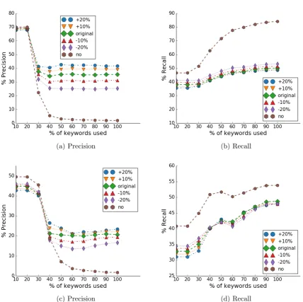
After having evaluated our methods and compared them with the state-of-the-art when answering to all the queries, we evaluated our methods when using a dynamically defined similarity threshold. The threshold we have chosen to use are automatically calculated by the results of the 4-hour timeslots of the previous days. As a result, we have 6 user-free dynamic thresholds that are calculated by taking the mean of the mean similarities of the previous respective timeslots. By introducing the thresholds in our methods, we answer to less query-tweets, reducing the recall but increasing the precision up to 100%. In Figure 3.3, we present the precisions and the recalls after the introduction of the thresholds for the method TG-C, while in Figure 3.4 we present the precision and recall for TG-TI-C. We run experiments by using no threshold, the exact dynamic threshold, and the exact threshold +-10% and +-20%. Furthermore, in order to evaluate the results, we use the balanced F1-measure. The results of the F1 measure for the two methods presented before is depicted in Figure 3.5.
(a) Precision (b) Recall
Figure 3.3: Precision and recall on Neighbourhood Level for TG when using dynamic thresholds (Th) (@Top1 and @0-Step).
(a) Precision (b) Recall
Figure 3.4: Precision and recall on Neighbourhood Level for TG-TI-C when using dynamic
(a) TG (b) TG-TI-C
Figure 3.5: F1 measure for Neighbourhood Level without and with threshold (Th) (@Top1 and
@0-Step).
the keywords for both cases. On the contrary, at the city-level analysis, the TG-TI and TG-TI-C algorithms are always better when compared to TG.
(a) @Top3 (b) @Top5
Figure 3.6: Accuracy for Neighbourhood Level for TG, TG-C, TG-TI, and TG-TI-C (@0-Step).
(a) TG (b) TG-C
(c) TG-TI (d) TG-TI-C
3.4.2 Evaluating the Algorithms with Linear Regression
Experimental Setup. We performed the experiments on a server running on Ubuntu 14.04.2 LTS, with 64GB RAM, and an Intel(R) Xeon(R) CPU E5506 @ 2.13GHz proces-sor. For the implementation of our methods and the reimplementation of the QL and KL we used Python 2.7.
Datasets. For the evaluation of our approach, we use 3 datasets containing geotagged1 posts from Twitter, generated in Italy, Germany and the Netherlands. In particular, we have data from 6 of the largest Italian cities, namely, Rome, Milan, Naples, Bologna, Venice and Turin, and from the capital of Germany, Berlin, and the capital of Netherlands, Amsterdam. The tweets from Italy were generated between June 20 and July 23, 2014, while the tweets from Germany and the Netherlands were generated between August 10 and September 11, 2014. The granularity of the neighborhood level we use for every city is a square with side of 1000 meters. The number of tweets is 543.295 for Italy (219.681 originated from Rome, 137.622 from Milan, 60.065 from Naples, 49.434 from Bologna, 46.982 from Turin, and 29.511 from Venice), 77.179 for Berlin and 136.189 for Amsterdam. The time windows we use have a duration of 4 hours (which can effectively capture an important event, as well as the start and the aftermath of this event), while also keeping the detailed aggregated information for every 15min time interval. As mentioned in Section 3.3.5, we use the sliding window model. We experimented sliding the window by 1 and by 2 time intervals, getting almost the same results; thus, we chose to slide our window by 2 time intervals per slide (30-minutes), which led to faster execution times. Finally, the default grid we use in this study is 20 by 20 squares.
Algorithms. We experimentally evaluate the six one-level algorithms we described in Section 3.3, namely, TG, TG-TI, TG-C, TG-TI-C, TG-CLR and TG-TI-CLR (the last two only for the neighborhood level). As baselines, we implemented the QL and KL methods [37], which