R E S E A R C H A R T I C L E
Open Access
A novel gene selection algorithm for cancer
classification using microarray datasets
Russul Alanni
*, Jingyu Hou, Hasseeb Azzawi and Yong Xiang
Abstract
Background:Microarray datasets are an important medical diagnostic tool as they represent the states of a cell at the molecular level. Available microarray datasets for classifying cancer types generally have a fairly small sample size compared to the large number of genes involved. This fact is known as a curse of dimensionality, which is a challenging problem. Gene selection is a promising approach that addresses this problem and plays an important role in the development of efficient cancer classification due to the fact that only a small number of genes are related to the classification problem. Gene selection addresses many problems in microarray datasets such as reducing the number of irrelevant and noisy genes, and selecting the most related genes to improve the classification results.
Methods: An innovative Gene Selection Programming (GSP) method is proposed to select relevant genes for
effective and efficient cancer classification. GSP is based on Gene Expression Programming (GEP) method with a new defined population initialization algorithm, a new fitness function definition, and improved mutation and recombination operators. . Support Vector Machine (SVM) with a linear kernel serves as a classifier of the GSP.
Results: Experimental results on ten microarray cancer datasets demonstrate that Gene Selection
Programming (GSP) is effective and efficient in eliminating irrelevant and redundant genes/features from microarray datasets. The comprehensive evaluations and comparisons with other methods show that GSP gives a better compromise in terms of all three evaluation criteria, i.e., classification accuracy, number of selected genes, and computational cost. The gene set selected by GSP has shown its superior performances in cancer classification compared to those selected by the up-to-date representative gene selection methods.
Conclusion: Gene subset selected by GSP can achieve a higher classification accuracy with less processing
time.
Keywords: Gene selection, Gene expression programming, Support vector machine, Microarray cancer dataset
Background
The rapid development of microarray technology in the past few years has enabled researchers to analyse thou-sands of genes simultaneously and obtain biological in-formation for various purposes, especially for cancer classification. However, gene expression data obtained by microarray technology could bring difficulties to clas-sification methods due to the fact that usually the num-ber of genes in a microarray dataset is very big, while the number of samples is small. This fact is known as
the curse of dimensionality in data mining [1–4]. Gene selection, which extracts informative and relevant genes, is one of the effective options to over-come the curse of dimensionality in microarray data based cancer classification.
Gene selection is actually a process of identifying a subset of informative genes from the original gene set. This gene subset enables researchers to obtain substan-tial insight into the genetic nature of the disease and the mechanisms responsible for it. This technique can also decrease the computational costs and improve the can-cer classification performance [5,6].
* Correspondence:[email protected]
School of Information Technology, Deakin University, Burwood 3125, VIC, Australia
Typically, the approaches for gene selection can be classified into three main categories: filter, wrapper and embedded techniques [6, 7]. The filter technique ex-ploits the general characteristics of the gene expressions in the dataset to evaluate each gene individually with-out considering classification algorithms. The wrapper technique is to add or remove genes to produce sev-eral gene subsets and then evaluates these subsets by using the classification algorithms to obtain the best gene subset for solving the classification problem. The embedded technique is between the filter and wrapper techniques in order to take advantage of the merits of both techniques. However, most of the em-bedded techniques deal with genes one by one [8], which is time consuming especially when the data di-mension is large such as the microarray data.
Naturally inspired evolutionary algorithms are more applicable and accurate than wrapper gene selection methods [9, 10] due to their ability in searching for the optimal or near-optimal solutions on large and complex spaces of possible solutions. Evolutionary algorithms also consider multiple attributes (genes) during their search for a solution, instead of considering one attribute at a time.
Various evolutionary algorithms [11–19] have been proposed to extract informative and relevant cancer genes and meanwhile reduce the number of noise and irrelevant genes. However, in order to obtain high ac-curacy results, most of these methods have to select a large number of genes. Chuang et al. [20] proposed the improved binary particle swarm optimization (IBPSO) method which achieved a good accuracy for some datasets but, again, selected a large number of genes. An enhancement of BPSO algorithm was pro-posed by Mohamad et al. [21] by minimizing the number of selected genes. They obtained good classi-fication accuracies for some datasets, but the number of selected genes is not small enough compared with other studies.
Recently, Moosa et al. [22] proposed a modified Artificial Bee Colony algorithm (mABC). Another study [15] proposed a hybrid method by using Infor-mation Gain algorithm to reduce the number of irrelevant genes and using an improved simplified swarm optimization (ISSO) to select the optimal gene subset. These two studies were able to get a good accuracy with small number of selected genes. However, the number of selected genes is still high compared with our method.
In recent years, a new evolutionary algorithm known as Gene Expression Programming (GEP) was initially in-troduced by Ferreira [23] and widely used in many appli-cations for classification and decision making [24–30]. GEP has three main advantages
– Flexibility, which makes it easy to design an optimal model. In other words, any part of GEP steps can be improved or changed without adding any complexity to the whole process.
– The power of achieving the target that is inspired from the ideas of genotype and phenotype
– Data visualization. It is easy to visualize each step of the GEP and that distinguishes it from many algorithms
These advantages make it easy to use GEP process to create our new gene selection program and simulate the dynamic process of achieving the optimal solution in de-cision making.
A few studies applied GEP as a feature selection method and obtained some promising results [31, 32] which encourage us to do further research.
GEP algorithm, based on its evolutionary structure, faces some computational problems, when it is applied to complex and high dimensional data such as micro-array datasets. Inspired by the above circumstances, to enhance the robustness and stability of microarray data classifiers, we propose a novel gene selection method based on the improvement of GEP. This proposed algo-rithm is called Gene Selection Programming (GSP). The idea behind this approach is to control the GEP solution process by replacing the random adding, deleting and selection with the systematic gene-ranking based se-lection. In this paper four innovative operations are presented: attributes/genes selection (initializing the population), mutation operation, recombination oper-ation and a new fitness function. More details of GSP are presented in the Methods section.
In this work, support vector machine (SVM) with a linear kernel serves to evaluate the performance of GSP. For a better reliability we used leave-one-out cross valid-ation (LOOCV). The results were evaluated in terms of three metrics: classification accuracy, number of selected genes and CPU time.
The rest of this paper is organized as follows: The overview of GEP and the proposed gene selection algo-rithm GSP are presented in theMethodssection (section 2). Resultssection (section 3) provides the experimental results on ten microarray datasets. Discussion section (section 4) presents the statistical analysis and discussion about the experimental results. Finally, Conclusion sec-tion (secsec-tion 5) gives the conclusions and direcsec-tions of future research.
Methods
Gene expression programming
(genotype), which are composed of one or more genes. Each gene consists of a head and a tail. The head may contain functional elements like {Q, +, −, ×, /} or terminal elements, while the tail contains ter-minals only. The terter-minals represent the attributes in the datasets. In this study, sometimes we use the term attribute to represent the gene in microarray dataset to avoid the possible confusion between the gene in microarray datasets and the gene in GEP chromosome. The size of the tail (t) is computed as t = h (n-1) + 1, where h is the head size, and n is the maximum number of parameters required in the function set. The second part of GEP is a phenotype which is a tree structure also known as expression tree (ET). When the representation of each gene in the chromosome is given, the genotype is established. Then the genotype can be converted to the phenotype by using specific languages invented by the GEP author.
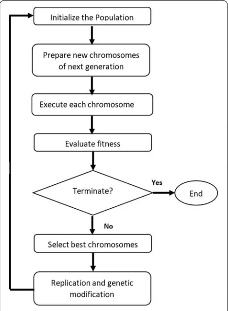
GEP process has four main steps: initialize the popula-tion by creating the chromosomes (individuals), identify a suitable fitness function to evaluate the best individual, conduct genetic operations to modify the individuals
to achieve the optimal solution in the next
generation, and check the stop conditions. GEP flow-chart is shown in Fig. 1.
It is worth mentioning that the GEP algorithm faces some challenging problems, especially the computational efficiency, when it is applied on the
complex and high-dimensional data such as a
microarray dataset. This motivates us to solve these problems and further improve the performance of the GEP algorithm by improving the evolution process. The details of the proposed gene selection programming (GSP) algorithm, which is based on GEP, for cancer classification are given in the fol-lowing sub-sections.
Systematic selection approach to initial GSP population
Initializing population is the first step in our gene se-lection method for which candidates are constructed from two sets: terminal set (ts) and function set (fs). Terminal set should represent the attributes of the microarray dataset. The question is what attributes should be selected into the terminal set. Selecting all attributes (including the unrelated attributes) will affect the computational efficiency. The best way to reduce the noise from the microarray data is to minimize the number of unrelated genes. There are two commonly used ways to do that: either by identi-fying a threshold and the genes ranked above a threshold are selected, or by selecting the n-top ranked genes (e.g. top 50 ranked genes). Both ways have disadvantages: defining a threshold suitable for different datasets is very difficult and deciding how many genes should be selected is subjective. To avoid these disadvantages, we use a different technique named systematic selection approach.
The systematic selection approach consists of three steps: rank all the attributes, calculate the weight of each attribute, and select the attributes based on their weight using the Roulette wheel selection method. The details of these steps are shown in the following sub-sections.
Attribute ranking
We use the Information Gain (IG) algorithm [33] to rank the microarray attributes. IG is a filter method mainly used to rank and find the most relevant genes [15, 34, 35]. The attributes with a higher rank value have more impact on the classification process, while the attributes with a zero rank value are considered irrelevant. The rank values of all attributes are calcu-lated once and saved in the buffer for later use in the program.
Weight calculation
The weight (w) of each attribute (i) is calculated based on Eq (1)
wi¼sumri ∈½0;1 ð1Þ
where sum¼Piri ∀i∈ts and r is the rank value, and P
iwi¼1.
The attributes with a higher weight contain more in-formation about the classification.
Attribute selection
In our systematic selection approach, we use the Roulette wheel selection method, which is also known as proportionate selection [36], to select the strong attributes (i.e., the attributes with a high weight). With this approach all the attributes are placed on the roulette wheel according to their weight. An attribute with a higher weight has a higher probability to be selected as a ter-minal element. This approach could reduce the number of irrelevant attributes in the final ter-minal set. The population is then initialized from this final terminal set (ts) and the function set (fs).
Each chromosome (c) in GSP is encoded with the length of N*(gene_length), where N represents the number of genes in each chromosome (c) and the length of a gene (g) is the length of its head (h) plus the length of its tail (t). In order to set the effective chromosome length in GSP, we need to determine the head size as well as the number of genes in each chromosome (details are in the Results section). The process of creating GSP chromosomes is illustrated in Algorithm 1
Fitness function design
The objective of the gene selection method is to find the smallest subset of genes that can achieve the highest accuracy. To this end, we need to de-fine a suitable fitness function for GEP that has the ability to find the best individuals/chromosomes.
We define the fitness value of an individual chromosome i as follow:
fi¼2rAC ið Þ þrt−tsi ð2Þ
This fitness function consists of two parts. The first part is based on the accuracy resultAC(i). This accuracy is measured based on the support vector machine (SVM) classifier using LOOCV.
For example, if chromosomeiis +/Qa2a1a5a6a3,its ex-pression tree (ET) is
Then, the input values for the SVM classifier are the attributes a2, a1and a5.
The second part of the fitness function is based on the number of the selected attributes si in the individual
chromosome and the total number tof attributes in the dataset . Parameterris a random value within the range (0.1, 1) giving an importance to the accuracy with respect to the number of attributes. Since the accuracy value is more important than the number of selected attributes in measuring the fitness of a chromosome, we multiply the accuracy by 2r.
Improved genetic operations
The purpose of the genetic operations is to improve the individual chromosomes towards the optimal solution. In this work, we improve two genetic operations as shown below.
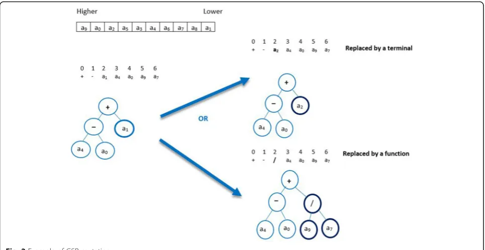
Mutation
Mutation is the most important genetic operator. It makes a small change to the genomes by replacing an element with another. The accumulation of several changes can create a significant variation. The random mutation may result in the loss of the important attri-butes, which may reduce the accuracy and increase the processing time.
In the example, the chromosome c has one gene. The head size is 3, so the tail length is h (n-1) + 1=4 and the chromosome length is (3+4) =7. The weight table shows that the attribute with the highest weight in the chromo-some is a9and the attribute with the lowest weight is a1. With the mutation GSP method selects the weakest ter-minallt(the terminal with lowest weight) which is a1in our example. There are two options to replace a1: the program could select either a function such as (/) or a terminal to replace it. In the latter option, the terminal should have a weight higher than that of a1, and the fit-ness value of the new chromosome c` must be higher than the original one. This new mutation operation is outlined in Algorithm 2.
Recombination
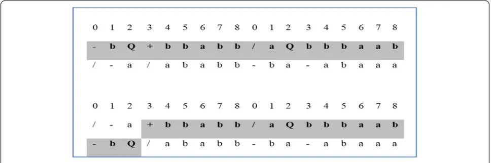
The second operation that we use in our gene se-lection method is the recombination operation. In recombination, two parent chromosomes are ran-domly chosen to exchange some material (short se-quence) between them. The short sequence can be one or more elements in a gene (see Fig. 3). The two parent chromosomes could also exchange an entire gene in one chromosome with another gene in another chromosome.
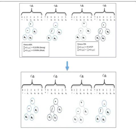
In this work, we improve the gene recombination by controlling the exchanging process. Suppose c1and c2 are two chromosomes (see Fig.4). The fitness value of c1 = 80% and the fitness value of c2 = 70% based on our fitness function (2). We select the “strong” gene (the one with the highest weight summation) from the chromosome that has the lowest fitness value (lc) and exchange it with the “weak” gene (the one with the lowest weight summation) from another chromo-some that has the highest fitness value (hc). In gen-eral, this process increases the fitness of hc. We repeat the exchange process until we get a new chromosome (hc’) with a higher fitness value than that of both parent chromosomes. The hc` has a higher probability of being a transcription in the next generation. This idea comes from the gene structure [37].
Based on the above innovative improvements for the GSP method in this section, we present the steps of GSP in Algorithm 3 with pseudocode.
Results
In this section, we evaluate the performance of GSP method using ten microarray cancer datasets, which were downloaded from http://www.gems-system.org. Table1 presents the details of the experimental datasets in terms of diverse samples, attributes and classes.
Our experimental results contain three parts. Part 1 (Ev.1) evaluated the best setting for GSP based on the number of genes (g) in each chromosome and the head size (h). Part 2 (Ev.2) evaluated the GSP performance in terms of three metrics: classification accuracy, number
of selected genes and CPU Time. To guarantee the impartial classification results and avoid generating bias results, this study adopted cross validation method LOOCV to reduce the bias in evaluating their perform-ance over each dataset. Our gene selection results were compared with three gene selection methods using the same classification model for the sake of fair competi-tion. Part 3 (Ev.3) evaluated the overall GSP perform-ance by comparing it with other up-to-date models.
Ev.1 the best setting for gene and head
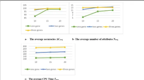
To set the best values for the number of genes (g) of each chromosome and the size of the gene head (h) in the GSP method, we evaluated nine different settings to show their effect on the GSP performance results. For g we selected three values 1, 2 and 3, and for each g value we selected three h values: 10, 15 and 20. We increased the values of h by 5 to make it clear to observe the effect of h values on the GSP performance, especially when the effect of increasing h is very slight. For more reliability, we used three different datasets (11_Tumors, Leukaemia 1, Prostate Tumor). The parameters used in GSP are listed in Table2.
The average results across the three experimental datasets are presented in Table 3. ACavg, Navg and Tavg represent the average accuracy, number of selected attri-butes and CPU time respectively for ten runs, while ACstd, , Nstd. and Tstd. represent the standard deviation for the classification accuracy, number of selected attri-butes and CPU time respectively.
Figure 5 shows the evaluation values in terms of ACavg, Tavg. and Navg for three different numbers of genes in each chromosome.
It is observed from the results in Table3that:
1- Comparing g with h: g has a stronger effect on the results than h.
Fig. 4Example for GSP Recombination
Table 1Description of the experimental datasets
No. Dataset Samples Attributes Classes Reference
1 11_Tumors 174 12533 11 [38]
2 9_Tumors 60 5726 9 [39]
3 Brain_Tumor1 90 5920 5 [40]
4 Brain_Tumor2 50 10367 4 [41]
5 Leukemia 1 72 5327 3 [42]
6 Leukemia 2 72 11225 3 [43]
7 Lung_Cancer 203 12600 5 [44]
8 SRBCT 82 2308 4 [45]
9 Prostate_Tumor 102 10509 2 [46]
10 DLBCL 77 5469 2 [47]
Table 2Parameters used in GSP
Parameter Setting
Function set +, -, ÷,Q
Terminal set Selected informative genes from the microarray dataset using systematic selection.
Number of chromosomes 200
Maximum Number of generations 2000
Genetic operators
Mutation 0.044
2- Regarding g results: when g was increased, ACavg,
TavgandNavgwere increased as well (positive
relationships). The results ofACstd,, Tstd.andNstd.
were decreased when g was increased (negative relationships). The results became stable when the g value was greater than 2.
3- Regarding h results: h has positive relationships withACavg, Tavgand Navgand negative relationships
withACstd,, Tstd.and Nstd. The results became
stable when the h value was over 15.
4- Increasing h values would increase the complexity of the model while theACandNresults would not show a notable enhancement.
5- The best setting for g and h was 2 and 15 respectively.
Ev.2: Comparison of the GSP performance with representative gene selection algorithms
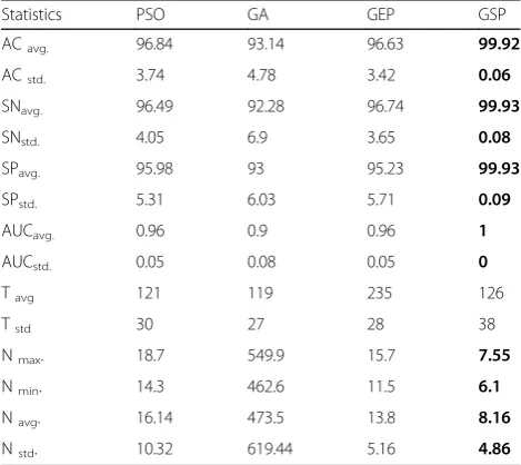
In order to evaluate the performance of our GSP algo-rithm objectively, we first evaluated its performance in terms of three evaluation criteria: classification accur-acy (AC), number of selected attributes (N) and CPU Time (T). Then we compared the results with three popular gene selection algorithms named Particle Swarm Optimization (PSO) [48], GEP and GA [49] using the same model for the sake of a fair compari-son. The parameters of the comparison methods are listed in Table 4.
The Information Gain algorithm was used in order to filter irrelevant and noisy genes and reduce the compu-tational load for the gene selection and classification methods.
The support vector machine (SVM) with a linear kernel served as a classifier of these gene selection methods. In order to avoid selection bias, the LOOCV was used. Weka
Table 3The results of different setting for g and h. Bold font indicates the best results
g h ACavg ACstd Navg Nstd Tavg Tstd
1 10 87.587 3.423 5.567 2.16 151.1202 0.00594
15 94.787 2.757 10.067 1.977 154.1243 0.00334
20 96.317 2.147 11 1.6 157.7917 0.00277
average 92.897 2.776 8.878 1.912 154.3454 0.004016
2 10 97.453 1.033 11.633 1.637 266.7896 0.00162
15 99.543 0.183 13.267 0.973 275.1234 0.00146
20 99.543 0.183 13.633 0.987 280.1246 0.00149
average 98.847 0.467 12.844 1.199 274.0125 0.001522
3 10 98.397 0.853 13.133 0.9737 381.0373 0.00445
15 99.21 0.19 13.3 0.973 382.3714 0.00143
20 99.21 0.177 13.3 0.973 388.7084 0.00133
average 98.939 0.407 13.244 0.973 384.039 0.002404
software was used to implement the PSO and GA models with default settings, while the GEP model was imple-mented by using java package GEP4J [50]. Table5shows the comparison results of GSP with three gene selection algorithms across ten selected datasets.
The experimental results showed that the GSP algo-rithm achieved the highest average accuracy result (99.92%) across the ten experimental datasets, while the average accuracies of other models were 97.643%, 97.886% and 94.904% for GEP, PSO and GA respectively.
The standard deviation results showed that GSP had the smallest value (0.342671), while the average standard deviations were3.425399, 3.3534102 and 5.24038421 for GEP, PSO and GA respectively. This means the GSP algorithm made the classification performance more accurate and stable.
The GSP algorithm achieved the smallest number of predictive/relevant genes (8.16), while the average num-ber of predictive genes was 13.8, 16.14 and 473.5 for GEP, PSO and GA respectively.
These evaluation results show that GSP is a promising approach for solving gene selection and cancer classifica-tion problems.
CPU Time results showed that GSP took almost half of the time that GEP needed to achieve the best solu-tion. However, the time is still long compared with the PSO and GA methods.
Ev.3: Comparison of GSP with up-to-date classification models
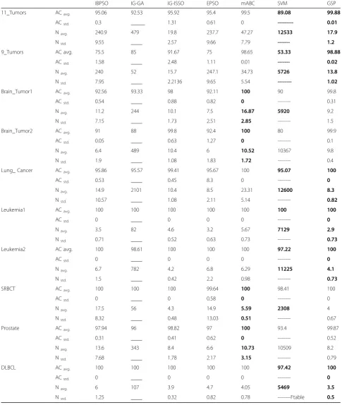
For more evaluations, we compared our GSP model with up-to-date classification models IBPSO, SVM [14], IG-GA [35], IG-ISSO [15], EPSO [21] and mABC [22]. This comparison was based on the classification result and the number of genes regardless of the methods of data processing and classification. The comparison re-sults on ten datasets are presented in Table6.
It can be seen from Table6that GSP performed better than its competitors on seven datasets (11_Tumors, 9_Tumors, Lung_ Cancer, Leukemia1, Leukemia2, SRBCT, and DLBCL), while mABC had better results on three data sets (Brain_Tumor1, Brain_Tumor2, and Prostate).
Interestingly, all runs of GSP achieved 100% LOOCV accuracy with less than 5 selected genes on the Lung_Cancer, Leukemia1, Leukemia2, SRBCT, and DLBCL datasets. Moreover, over 98% classification accuracies were obtained on other datasets. These results indicate that GSP has a high potential to achieve the ideal solution with less number of genes, and the selected genes are the most rele-vant ones.
Regarding the standard deviations in Table 6, re-sults that produced by GSP were almost consistent on all datasets. The differences of the accuracy re-sults and the number of genes in each run were very small. For GSP, the highest ACstd was 0.52 while the highest Nstd was 1.5. This means that GSP has a stable process to select and produce a near-optimal gene subset from a high dimensional dataset (gene expression data).
Discussion
We applied GSP method on ten microarray datasets. The results of GSP performance evaluations show that GSP can generate a subset of genes with a very small number of related genes for cancer classification on each dataset. Across the ten experimental datasets, the max-imum number of selected genes is 17 with the accuracy not less than 98.88%.
The performance results of GSP and other compara-tive models (see Table 6) on Prostate and Brain tumor datasets were not as good as the results on other data-sets. This is probably due to the fact that these models concentrated on reducing the number of irrelevant genes, but ignored other issues such as the missing values and redundancy. More effort needs to be made
Table 4Parameter setting of the competitors
GA GEP PSO
Parameters Values Parameters Values Parameters Values
#chromosomes 200 #chromosomes 200 # particles 200
# generations 2000 # generations 2000 # iterations 2000
Crossover rate 0.8 Crossover rate 0.8 Weight (w) 0.8
mutation rate 0.1 mutation rate 0.1 Accelerations c1 and c2
2
Table 5Comparison of GSP with three gene selection algorithms on ten selected datasets. Bold font indicates the best results
Statistics PSO GA GEP GSP
ACavg. 96.84 93.14 96.63 99.92
ACstd. 3.74 4.78 3.42 0.06
SNavg. 96.49 92.28 96.74 99.93
SNstd. 4.05 6.9 3.65 0.08
SPavg. 95.98 93 95.23 99.93
SPstd. 5.31 6.03 5.71 0.09
AUCavg. 0.96 0.9 0.96 1
AUCstd. 0.05 0.08 0.05 0
Tavg 121 119 235 126
Tstd 30 27 28 38
Nmax. 18.7 549.9 15.7 7.55
Nmin. 14.3 462.6 11.5 6.1
Navg. 16.14 473.5 13.8 8.16
on microarray data processing before applying the GSP model to achieve better results.
The GSP method on datasets 11_Tumors and 9_Tu-mors achieved relatively lower accuracy results (99.88%
and 98.88% respectively) compared with the accuracy re-sults on other datasets. The reason was due to the high number of classes (11 and 9 respectively) which could be a problem to any classification models.
Table 6Comparison of the gene selection algorithms on ten selected datasets. Bold font indicates the best results
IBPSO IG-GA IG-ISSO EPSO mABC SVM GSP
11_Tumors ACavg. 95.06 92.53 95.92 95.4 99.5 89.08 99.88
ACstd. 0.3 _____ 1.31 0.61 0 --- 0.01
Navg. 240.9 479 19.8 237.7 47.27 12533 17.9
Nstd. 9.55 ____ 2.57 9.66 7.79 --- 1.2
9_Tumors AC avg. 75.5 85 91.67 75 98.65 53.33 98.88
ACstd. 1.58 ____ 2.48 1.11 0.01 --- 0.02
Navg. 240 52 15.7 247.1 34.73 5726 13.8
Nstd. 7.95 ____ 2.2136 9.65 5.54 --- 1.02
Brain_Tumor1 ACavg. 92.56 93.33 98 92.11 100 90 99.8
ACstd. 0.54 ____ 0.88 0.82 0 --- 0.31
Navg. 11.2 244 10.1 7.5 16.87 5920 9.2
Nstd. 7.15 ____ 1.73 2.51 2.85 --- 1.5
Brain_Tumor2 ACavg. 91 88 99.8 92.4 100 80 99.9
ACstd. 0.05 ____ 0.63 1.27 0 --- 0.1
Navg. 6.4 489 10.4 6 10.52 10367 9.8
Nstd. 1.9 ____ 1.08 1.83 1.72 --- 0.4
Lung_ Cancer ACavg. 95.86 95.57 99.41 95.67 100 95.07 100
ACstd. 0.53 ____ 0.45 8.3 0 --- 0
Navg. 14.9 2101 10.4 8.5 23.31 12600 8.3
Nstd. 10.57 ____ 1.08 2.11 5.14 --- 0.82
Leukemia1 ACavg. 100 100 100 100 100 100 100
ACstd. 0 ____ 0 0 0 --- 0
Navg. 3.5 82 4.6 3.2 5.67 7129 2.9
Nstd. 0.71 ____ 0.52 0.63 0.73 --- 0.73
Leukemia2 AC avg. 100 98.61 100 100 100 97.22 100
ACstd. 0 ____ 0 0 0 --- 0
Navg. 6.7 782 4.2 6.8 6.29 11225 4.1
Nstd. 1.5 ____ 0.42 2.2 0.98 --- 0.73
SRBCT ACavg. 100 100 100 99.64 100 98.41 100
ACstd. 0 ____ 0 0.58 0 --- 0
Navg. 17.5 56 4.3 14.9 5.59 2308 4
Nstd. 8.32 ____ 0.48 13.03 0.51 --- 0.67
Prostate ACavg. 97.94 96 98.82 97 100 93.4 99.87
ACstd. 0.31 ____ 0.41 0.62 0 --- 0.52
Navg. 13.6 343 8.4 6.6 10.73 10509 8.2
Nstd. 7.68 ____ 1.78 2.17 3.15 --- 0.79
DLBCL ACavg. 100 100 100 100 100 97.42 100
ACstd. 0 ____ 0 0 0 --- 0
Navg. 6 107 3.9 4.7 4.05 5469 3.5
We noticed from GSP performance that when the ac-curacy increased the number of selected genes and the processing time decreased (negative relationship). This proves that GSP is effective and efficient for gene selec-tion method.
Conclusions
In this study, we have proposed an innovative gene se-lection algorithm (GSP). This algorithm can not only provide a smaller subset of relevant genes for cancer classification but also achieve higher classification accuracies in most cases with shorter processing time compared with GEP. The comparisons with the repre-sentative state-of-art models on ten microarray datasets show the outperformance of GSP in terms of classifica-tion accuracy and the number of selected genes. How-ever, the processing time of GSP is still longer than that of PSO and GA models. Our future research direction is to reduce the processing time of GSP while still keeping the effectiveness of the method.
Abbreviations
AC:Accuracy; ACavg: The average value of accuracy; BPSO: Binary Particle Swarm Optimization; c: Chromosome; ET: Expression Tree; fs: Function set; GA: Genetic Algorithm; GEP: Gene Expression Programming; GSP: Gene Selection Programming; h: Head; IBPSO: Improved Binary Particle Swarm Optimization; ISSO: Improved Simplified Swarm Optimization; LOOCV: Leave-one-out cross validation; mABC: Modified Artificial Bee Colony algorithm; N: Number of genes in each chromosome; Navg: The average number of selected attributes; PSO: Particle Swarm Optimization; r: Rank value; SVM: Support Vector Machine; t: Tail; Tavg: The average value of CPU time; TS: Tabu Search; Ts: Terminal set; w: Weight
Acknowledgements
We appreciate Deakin University staff for their continued cooperation. We thank Rana Abdul jabbar for the guidance on data analysis.
Funding
No funding was received
Availability of data and materials
All the datasets were downloaded fromhttp://www.gems-system.org.
Authors’contributions
RA designed the study, wrote the code and drafted the manuscript, JH designed the model and the experiments and revised the manuscript. HA and YX participated in the model design and coordination, and helped to draft the manuscript. All authors read and approved the final manuscript.
Ethics approval and consent to participate Not applicable
Consent for publication Not applicable
Competing interests
The authors declare that they have no competing interests.
Publisher’s Note
Springer Nature remains neutral with regard to jurisdictional claims in published maps and institutional affiliations.
Received: 27 September 2018 Accepted: 7 December 2018
References
1. Wang H-Q, Jing G-J, Zheng C. Biology-constrained gene expression discretization for cancer classification. Neurocomputing. 2014;145:30–6.
2. Espezua S, Villanueva E, Maciel CD, Carvalho A. A Projection Pursuit framework for supervised dimension reduction of high dimensional small sample datasets. Neurocomputing. 2015;149:767–76.
3. Seo M, Oh S. A novel divide-and-merge classification for high dimensional datasets. Comput Biol Chem. 2013;42:23–34.
4. Xie H, Li J, Zhang Q, Wang Y. Comparison among dimensionality reduction techniques based on Random Projection for cancer classification. Comput Biol Chem. 2016;65:165–72.
5. Tabakhi S, Najafi A, Ranjbar R, Moradi P. Gene selection for microarray data classification using a novel ant colony optimization. Neurocomputing. 2015; 168:1024–36.
6. Du D, Li K, Li X, Fei M. A novel forward gene selection algorithm for microarray data. Neurocomputing. 2014;133:446–58.
7. Mundra PA, Rajapakse JC. Gene and sample selection for cancer classification with support vectors based t-statistic. Neurocomputing. 2010;73:2353–62. 8. Jin C, Jin S-W, Qin L-N. Attribute selection method based on a hybrid BPNN
and PSO algorithms. Appl Soft Comput. 2012;12:2147–55. 9. Alshamlan H, Badr G, Alohali Y. mRMR-ABC: A Hybrid Gene Selection
Algorithm for Cancer Classification Using Microarray Gene Expression Profiling. Biomed Res Int. 2015;2015:604910.
10. Alshamlan HM, Badr GH, Alohali YA. The performance of bio-inspired evolutionary gene selection methods for cancer classification using microarray dataset. Int J Biosci, Biochem Bioinformatics. 2014;4:166. 11. Azzawi H, Hou J, Alanni R, Xiang Y. SBC: A New Strategy for Multiclass Lung
Cancer Classification Based on Tumour Structural Information and Microarray Data.In 2018 IEEE/ACIS 17th International Conference on Computer and Information Science (ICIS),2018: 68–73.
12. Chen K-H, Wang K-J, Tsai M-L, Wang K-M, Adrian AM, Cheng W-C, et al. Gene selection for cancer identification: a decision tree model empowered by particle swarm optimization algorithm. BMC Bioinformatics. 2014;15:1. 13. H. M. Zawbaa, E. Emary, A. E. Hassanien, and B. Parv, "A wrapper approach
for feature selection based on swarm optimization algorithm inspired from the behavior of social-spiders," in Soft Computing and Pattern Recognition (SoCPaR), 2015 7th International Conference of, 2015, pp. 25-30. 14. Mohamad MS, Omatu S, Deris S, Yoshioka M. A modified binary particle
swarm optimization for selecting the small subset of informative genes from gene expression data. IEEE Trans Inf Technol Biomed. 2011;15:813–22. 15. Lai C-M, Yeh W-C, Chang C-Y. Gene selection using information gain and
improved simplified swarm optimization. Neurocomputing. 2016;19;218: 331–8.
16. D. Karaboga and B. Basturk, "Artificial bee colony (ABC) optimization algorithm for solving constrained optimization problems," in International fuzzy systems association world congress, 2007, pp. 789-798.
17. Jain I, Jain VK, Jain R. Correlation feature selection based improved-Binary Particle Swarm Optimization for gene selection and cancer classification. Appl Soft Comput. 2018;62:203–15.
18. Pino Angulo A. Gene Selection for Microarray Cancer Data Classification by a Novel Rule-Based Algorithm. Information. 2018;9:6.
19. Chuang L-Y, Yang C-H, Yang C-H. Tabu search and binary particle swarm optimization for feature selection using microarray data. J Comput Biol. 2009;16:1689–703.
20. Chuang L-Y, Chang H-W, Tu C-J, Yang C-H. Improved binary PSO for feature selection using gene expression data. Comput Biol Chem. 2008;32:29–38. 21. Mohamad MS, Omatu S, Deris S, Yoshioka M, Abdullah A, Ibrahim Z. An
enhancement of binary particle swarm optimization for gene selection in classifying cancer classes. Algorithms Mol Biol. 2013;8:1.
22. Moosa JM, Shakur R, Kaykobad M, Rahman MS. Gene selection for cancer classification with the help of bees. BMC Med Genet. 2016;9:2–47. 23. Ferreira C. Gene expression programming in problem solving. In: Soft
computing and industry. London: Springer; 2002. p. 635–53.
24. Azzawi , Hou, J, Xiang Y, Alann R. Lung Cancer Prediction from Microarray Data by Gene Expression Programming. IET Syst Biol. 2016;10(5):168–78. 25. Yu Z, Lu H, Si H, Liu S, Li X, Gao C, et al. A highly efficient gene expression
26. Peng Y, Yuan C, Qin X, Huang J, Shi Y. An improved Gene Expression Programming approach for symbolic regression problems. Neurocomputing. 2014;137:293–301.
27. Kusy M, Obrzut B, Kluska J. Application of gene expression programming and neural networks to predict adverse events of radical hysterectomy in cervical cancer patients. Med Biol Eng Comput. 2013;51:1357–65. 28. Yu Z, Chen X-Z, Cui L-H, Si H-Z, Lu H-J, Liu S-H. Prediction of lung cancer
based on serum biomarkers by gene expression programming methods. Asian Pac J Cancer Prev. 2014;15:9367–73.
29. Al-Anni R, Hou J, Abdu-aljabar R, Xiang Y. Prediction of NSCLC recurrence from microarray data with GEP. IET Syst Biol. 2017;11(3):77–85. 30. Azzawi H, Hou J, Alanni R, Xiang Y, Abdu-Aljabar R, Azzawi A. Multiclass
Lung Cancer Diagnosis by Gene Expression Programming and Microarray Datasets. In: International Conference on Advanced Data Mining and Applications; 2017. p. 541–53.
31. Alsulaiman FA, Sakr N, Valdé JJ, El Saddik A, Georganas ND. Feature selection and classification in genetic programming: Application to haptic-based biometric data. In: Computational Intelligence for Security and Defense Applications, 2009. CISDA 2009. IEEE Symposium on; 2009. p. 1–7. 32. Alanni R, Hou J, Azzawi H, Xiang Y. New Gene Selection Method Using
Gene Expression Programing Approach on Microarray Data Sets. In: Lee R, editor. Computer and Information Science. Cham: Springer International Publishing; 2019. p. 17–31.
33. Y. Yang and J. O. Pedersen, "A comparative study on feature selection in text categorization," in Icml, 1997, pp. 412-420.
34. Dai J, Xu Q. Attribute selection based on information gain ratio in fuzzy rough set theory with application to tumor classification. Appl Soft Comput. 2013;13:211–21.
35. Yang C-H, Chuang L-Y, Yang CH. IG-GA: a hybrid filter/wrapper method for feature selection of microarray data. J Med Biol Eng. 2010;30:23–8. 36. Goldberg DE, Deb K. A comparative analysis of selection schemes used in
genetic algorithms. Found Genet Algorithms. 1991;1:69–93.
37. Suryamohan K, Halfon MS. Identifying transcriptional cis-regulatory modules in animal genomes. Wiley Interdiscip Rev Dev Biol. 2015;4:59–84. 38. Su AI, Welsh JB, Sapinoso LM, Kern SG, Dimitrov P, Lapp H, et al. Molecular
classification of human carcinomas by use of gene expression signatures. Cancer Res. 2001;61:7388–93.
39. Staunton JE, Slonim DK, Coller HA, Tamayo P, Angelo MJ, Park J, et al. Chemosensitivity prediction by transcriptional profiling. Proc Natl Acad Sci. 2001;98:10787–92.
40. Pomeroy SL, Tamayo P, Gaasenbeek M, Sturla LM, Angelo M, McLaughlin ME, et al. Prediction of central nervous system embryonal tumour outcome based on gene expression. Nature. 2002;415:436–42.
41. Nutt CL, Mani D, Betensky RA, Tamayo P, Cairncross JG, Ladd C, et al. Gene expression-based classification of malignant gliomas correlates better with survival than histological classification. Cancer Res. 2003;63:1602–7. 42. Golub TR, Slonim DK, Tamayo P, Huard C, Gaasenbeek M, Mesirov JP, et al.
Molecular classification of cancer: class discovery and class prediction by gene expression monitoring. Science. 1999;286:531–7.
43. Armstrong SA, Staunton JE, Silverman LB, Pieters R, den Boer ML, Minden MD, et al. MLL translocations specify a distinct gene expression profile that distinguishes a unique leukemia. Nat Genet. 2002;30:41–7.
44. Bhattacharjee A, Richards WG, Staunton J, Li C, Monti S, Vasa P, et al. Classification of human lung carcinomas by mRNA expression profiling reveals distinct adenocarcinoma subclasses. Proc Natl Acad Sci. 2001;98: 13790–5.
45. Khan J, Wei JS, Ringner M, Saal LH, Ladanyi M, Westermann F, et al. Classification and diagnostic prediction of cancers using gene expression profiling and artificial neural networks. Nat Med. 2001;7:673–9.
46. Singh D, Febbo PG, Ross K, Jackson DG, Manola J, Ladd C, et al. Gene expression correlates of clinical prostate cancer behavior. Cancer Cell. 2002;1:203–9.
47. Shipp MA, Ross KN, Tamayo P, Weng AP, Kutok JL, Aguiar RC, et al. Diffuse large B-cell lymphoma outcome prediction by gene-expression profiling and supervised machine learning. Nat Med. 2002;8:68–74.
48. Moraglio A, Di Chio C, Poli R. Geometric particle swarm optimisation. In: European conference on genetic programming; 2007. p. 125–36. 49. D. E. Goldberg, "Genetic algorithms in search, optimization and machine