S2P3-R (v1.0): a framework for efficient regional modelling of physical and biological structures and processes in shelf seas

www.geosci-model-dev.net/8/3163/2015/ doi:10.5194/gmd-8-3163-2015

© Author(s) 2015. CC Attribution 3.0 License.

S2P3-R (v1.0): a framework for efficient regional modelling of

physical and biological structures and processes in shelf seas

R. Marsh1, A. E. Hickman1, and J. Sharples2,3

1_{University of Southampton, National Oceanography Centre, Southampton, UK} 2_{School of Environmental Sciences, University of Liverpool, Liverpool L69 3BX, UK}

3_{National Oceanography Centre, Liverpool, Joseph Proudman Building, 6 Brownlow Street, Liverpool L3 5DA, UK}

Correspondence to: R. Marsh ([email protected])

Received: 17 December 2014 – Published in Geosci. Model Dev. Discuss.: 30 January 2015 Revised: 28 August 2015 – Accepted: 11 September 2015 – Published: 8 October 2015

Abstract. An established one-dimensional (1-D) model of Shelf Sea Physics and Primary Production (S2P3) is adapted for flexible use in selected regional settings over selected periods of time. This Regional adaptation of S2P3, the S2P3-R framework (v1.0), can be efficiently used to inves-tigate physical and biological phenomena in shelf seas that are strongly controlled by vertical processes. These include spring blooms that follow the onset of stratification, tidal mixing fronts that seasonally develop at boundaries between mixed and stratified water, and sub-surface chlorophyll max-ima that persist throughout summer. While not representing 3-D processes, S2P3-R reveals the horizontal variation of the key 1-D (vertical) processes. S2P3-R should therefore only be used in regions where horizontal processes – including mean flows, eddy fluxes and internal tides – are known to ex-ert a weak influence in comparison with vex-ertical processes. In such cases, S2P3-R may be used as a highly versatile research tool, alongside more complex and computationally expensive models. In undergraduate oceanography modules and research projects, the model serves as an effective prac-tical tool for linking theory and field observations. Three dif-ferent regional configurations of S2P3-R are described, il-lustrating a range of diagnostics, evaluated where practical with observations. The model can be forced with daily me-teorological variables for any selected year in the reanalysis era (1948 onwards). Example simulations illustrate the con-siderable extent of synoptic-to-interannual variability in the physics and biology of shelf seas. In discussion, the present limitations of S2P3-R are emphasised, and future develop-ments are outlined.

1 Introduction

In a global context, the shelf seas are disproportionately pro-ductive due to the continuous supply of nutrients (Holt et al., 2009a, and references therein). A variety of models have been developed to explore the processes that shape and main-tain productivity. Operational biogeochemistry and ecosys-tem models typically represent the sysecosys-tem with relatively high complexity and resolution, e.g. the 7 km Atlantic Mar-gin Model NEMO-ERSEM (AMM7-NE) system (Edwards et al., 2012) – see also http://www.metoffice.gov.uk/research/ news/marine-predictions. Such models may perform well alongside observations, but simulations rely on high perfor-mance computing resources such that extensive experimental work is consequently not practical.

between mixed and seasonally stratified water in mid-latitude shelf seas (Simpson and Hunter, 1974). While controlled to the first order by vertical processes, the transition from mixed to stratified water across a TMF typically occurs on a hori-zontal scale of ∼10–20 km (e.g. Moore et al., 2003); there-fore, for clear resolution of associated physical and biogeo-chemical structures, TMFs are ideally simulated at high hor-izontal resolution (1–2 km).

S2P3 was introduced as “PHYTO-1D” and originally de-scribed in Sharples (1999). An updated version of PHYTO-1D was described in Sharples (2008). The model is designed for use as an investigative (and educational) tool (see zipped material at http://pcwww.liv.ac.uk/~jons/model.htm). S2P3 has been used as a research tool to establish the varying in-fluence of winds and air–sea heat fluxes on inter-annual vari-ability in the timing of stratification and the spring bloom in the northwestern North Sea (Sharples et al., 2006), and to quantify the impact of spring–neap tidal cycles on biological productivity at TMFs (Sharples, 2008). In educational con-texts, S2P3 and forerunner models have been used for around 10 years in year 3 undergraduate and masters level postgrad-uate teaching at the Universities of Southampton and Liver-pool, in the UK.

In spite of potential for widespread application, S2P3 has not been extensively used and tested across real transects or in limited regions, where the model can be appropriately used for investigating time-evolving stratification and biological productivity. Introduced here, S2P3-R is a framework for us-ing S2P3 to efficiently model physical and biological struc-tures in shelf seas, for selected years during the reanalysis era (Kalnay et al., 1996). The development of S2P3-R has facili-tated the simulation of vertical processes and their horizontal variability in real time, for quick investigation of ongoing changes and detailed fieldwork planning.

In the remainder of the paper, we first outline the S2P3-R framework. We start with a brief description of the physical and biological components of S2P3, followed by details of the modified source code, model performance and diagnostic options. This is in turn followed by details on model set-up in different domains (horizontal meshes and tidal forcing), and the specification of meteorological forcing. We then evaluate model simulations for three different regions, undertaken and diagnosed using the new framework. In discussion, some im-portant caveats are emphasised, and we outline the prospects for development of the S2P3-R framework.

2 The S2P3-R framework 2.1 S2P3

Here, we provide a brief description of the physical and bio-logical components of S2P3, emphasising key equations. For a more detailed model description, the reader is referred to Sharples (1999, 2008).

2.1.1 Physical model

Central to the physics of S2P3 is a turbulence closure scheme, for which the prognostic variable is turbulent kinetic energy (TKE), formally defined asq2/2, whereq is the tur-bulent intensity, or velocity scale (m s−1). For a tidal current withx andy components uandv, the tendency of TKE is expressed as

∂ ∂t

_q2

2

= ∂

∂z

Kq ∂

∂z

_q2

2

+Nz "

∂u ∂z

2

+

_∂v

∂z

2#

+Kz

g ρ

∂ρ ∂z

− q 3

B1l

, (1)

where ρ is density, quadratic in temperature T (ρ= 1028.11−6.24956×10−2T −5.29468×10−3T2, assuming a constant salinity of 35.00), B1 is a constant of the clo-sure scheme,Kq is the vertical eddy diffusivity for TKE,

Kz is the vertical eddy diffusivity for other scalar proper-ties, Nz is vertical eddy viscosity, and l is an eddy length scale (l=κz(1−z/ h)0.5, at depthz, given total depthhand von Karmen’s constantκ=0.41). Forward time stepping is explicit throughout, with time steps,1t, constrained by the diffusive stability criterion,1t < 1z2/2Nz, given depth

in-tervals,1z.

Tides and winds force the TKE profile for given boundary conditions:

q_z2_=h=B₁2/3 τs ρz=h

, (2a)

q_z2₌₀=B₁2/3 τb ρz=0

, (2b)

whereτsis the surface (z=h)stress due to the wind, andτb is the near-bottom (z=0) stress due to tidal currents. Thex

andycomponents of wind stress are obtained as

τsx= −cdρauw

q u2

w+vw2

, (3a)

τsy= −cdρavw q

u2

w+vw2

(3b) given a drag coefficientcd(cd=(0.75+0.067w)×10−3, for wind speedw), air densityρa(=1.3 kg m−3), anduwandvw,

thexandycomponents of wind. Thexandycomponents of near-bottom stress are obtained as

τbx= −kbρ0u1

q

u2₁+v2₁

, (4a)

τby= −kbρ0v1

q

u2₁+v2₁ (4b)

In addition to mixing, the water column is locally heated and cooled. The tendency of temperature (T )is obtained at each depth level as

∂T

∂t =

∂ ∂z

Kz∂T

∂z

+Qh(z) , (5)

wherezis height above the seabed andQh(z)is the net heat-ing atz.

Heat fluxes are formulated as follows. We first define a surface net heat flux (Qnet)as the sum of incoming shortwave radiation (QSW), long-wave back radiation (QLW), and latent and sensible heat exchange with the atmosphere (Qsensand

Qlat):

Qnet=QSW−(QLW+Qsens+Qlat) . (6)

Incoming shortwave radiation, irradiance in the presence of clouds, is calculated as

QSW=

1.0−0.004C−0.000038C2QSW,c-s, (7) whereCis cloud fraction, and clear-sky irradiance,QSW,c-s, is obtained as

QSW,c-s=S (1−α) f (θ, t ) (1−κSW) , (8) where S is the solar constant (=1368 W m−2),α is an at-mospheric albedo (=0.24), f (θ, t )is a function represent-ing the daily and seasonal variation in day length at latitude

θ, andκSW is a shortwave absorption coefficient (=0.06). Long-wave radiation is calculated as

QLW=

εLW

1.0−0.6×10−4C2 0.39−0.05q0.5σ T4, (9) where εLW is long-wave emissivity (=0.985), q is vapour pressure (q=Rqs, given saturated vapour pressure qs(T ) and relative humidity R), and σ is the Stefan–Boltzmann constant (σ=5.67×10−8W m−2K−4). Sensible heat flux is calculated using the bulk formula

Qsens=ρacpChU (Ts−Ta) , (10)

where cp is the specific heat capacity of air (cp=

1004 J kg−1K−1),Ch is a transfer coefficient (Ch=1.45×

10−3),Uis surface wind speed,Tsis the sea surface temper-ature, and Ta is surface air temperature. Latent heat flux is calculated using the bulk formula

Qlat=ρaLvCeU (qs−q) , (11)

where Lv is the specific heat capacity of air (Lv=2.5×

106−2.3×103Ts), and Ce is a transfer coefficient (Ce=

1.5×10−3).

The surface net heat flux is partitioned down the water col-umn as follows. The red end of the spectrum, 55 % of short-wave radiation, is assumed to be absorbed at the top depth

level; hence, the surface heating,Qh,0=0.55QSW−(QLW+

Qsens+Qlat). The remaining 45 % of insolation is available for heating at lower levels, distributed exponentially through-out the water column as a heating rateQh(z), according to

∂Qh

∂z = −Qh(z) (λ0+εXT(z)) , (12)

whereλ0 is an attenuation coefficient (λ0=0.1 m−1) and

ε is a pigment absorption cross section (ε=0.012 m2 (mg chl)−1_{), accounting for shading due to XT(z), the} lo-cal chlorophyll a (chl a) concentration (mg chl m−3_), tak-ing XT(z)=qchlPC, for the cell chl a: carbon ratio, qchl (0.03 mg chl (mg C)−1), and carbon concentration, PC (see below).

2.1.2 Biological model

Phytoplankton is modelled in terms of an equivalent carbon concentration (PC; units mg C m−3)and internal cellular ni-trogen (PN). In each grid cell,PCtendency is due to the net effect of vertical mixing, growth and grazing, according to

∂PC

∂t =

∂ ∂z

Kz

∂PC

∂z

+µPC−GPC (13)

given a grazing impact rate,G, and a growth rate,µ, that is a function of photosynthetically active radiation:

µ=µm

1−e−(αIPARθ/µm)_−rB_{, (14)}

whereα is the maximum quantum yield,IPAR is the light availability,θis the chla: carbon ratio,rBis the respiration rate, and the maximum growth rate,µm, is given by

µm=1.16×10−5

_Q−Q

sub

Qm−Qsub

0.59e0.0633T, (15) whereQ=PN/PCis the cell nitrogen quota,Qsubis the sub-sistence nutrient : carbon quota, andQmis the maximum cell quota. The tendency for phytoplankton nitrogen (PN)is sim-ilarly described as

∂PN

∂t =

∂ ∂z

Kz

∂PN

∂z

+uPC−GPN, (16) where the uptake rateuis obtained as a Michaelis–Menton function of the dissolved inorganic nitrogen (DIN) concen-tration:

u=

um

1− Q

Qm

_DIN

(ku+DIN)

+

µQ, µ <0

0, µ≥0 (17) givenku, a half saturation coefficient for nutrient uptake, and

um, a maximum nutrient uptake rate. The uptake of nitrogen leads to a tendency in DIN:

∂DIN

∂t =

∂ ∂z

Kz

∂DIN

∂z

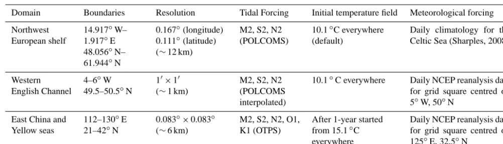
Table 1. Boundaries, resolution, tidal forcing, initial temperature and meteorological forcing for each domain (POLCOMS is Proudman Oceanographic Laboratory Coastal Ocean Modelling System; OTPS is OSU Tidal Prediction Software).

Domain Boundaries Resolution Tidal Forcing Initial temperature field Meteorological forcing

Northwest European shelf

14.917◦W– 1.917◦E 48.056◦N– 61.944◦N

0.167◦(longitude) 0.111◦(latitude) (∼12 km)

M2, S2, N2 (POLCOMS)

10.1◦C everywhere (default)

Daily climatology for the Celtic Sea (Sharples, 2008)

Western English Channel

4–6◦W 49.5–50.5◦N

10×10 (∼1 km)

M2, S2, N2 (POLCOMS interpolated)

10.1◦C everywhere Daily NCEP reanalysis data for grid square centred on 5◦W, 50◦N

East China and Yellow seas

112–130◦E 21–42◦N

0.083◦×0.083◦ (∼6 km)

M2, S2, N2, O1, K1 (OTPS)

After 1-year started from 15.1◦C everywhere

Daily NCEP reanalysis data for grid square centred on 125◦E, 32.5◦N

whereeis the fraction of grazed phytoplankton cellular ni-trogen recycled immediately back into the dissolved nini-trogen pool.

Water column nitrogen is constantly restored towards an initial winter concentration, DIN0(mmol m−3), by a flux of inorganic nitrogen from the seabed:

∂DIN1

∂t =

fDIN

1z

1−DIN1 DIN0

, (19)

where DIN1is the dissolved nitrogen in the bottom depth cell of the model grid,1z(m) is the thickness of the model grid cell, andfDIN (mmol m−2s−1)is the maximum flux of dis-solved nitrogen from the seabed into the bottom depth cell.

The values of biological parameters (G,µm,θ,rB,Qsub,

α,um, Qm, ku, e, DIN0, fDIN)are as listed in Table I of Sharples (2008).

2.2 Modified S2P3 source code, performance and diagnostics

For the S2P3-R framework, we modified the Fortran 90 source code of S2P3 v7.0, which includes additional com-mands and sub-routines to facilitate the Winteracter Fortran graphical user interface (GUI) toolset (Interactive Software Services Ltd., www.winteracter.com), the model being sup-plied with a text book (Simpson and Sharples, 2012) as an ex-ecutable application that runs under the Windows operating system. This source code was modified for compilation and execution in a Unix environment by removing GUI-related lines of code. These changes are solely to facilitate compi-lation and execution in Unix environments, and S2P3 is thus far unchanged as a scientific tool.

Within the new framework, S2P3 can be used to generate geographically specific maps, sections and time series, with varying run-time implications on a single processor. Maps typically comprise 5000–20 000 grid points, while sections comprise 10–100 grid points. For a given year (see below), maps can take over a day to generate (depending on the

ex-tent of shallower water, where shorter time steps are neces-sary), while sections typically take a few minutes, and annual time series at a single location typically take a few seconds.

Default mapped variables are the mid-summer surface– bottom temperature difference, annual-mean surface heat flux, and annual net production. Other quantities, such as the mid-summer sub-surface chla maximum (SCM) and SCM depth, can also be mapped. The option for simulating sec-tions is motivated by opportunities for direct comparison with measurements obtained through surveys and cruises. In selecting to simulate section data, constant depth intervals are specified for plotting on a regular distance–depth mesh without the need for interpolation. The option for time series at single locations is motivated by the availability of time series at repeat conductivity–temperature–depth (CTD) sta-tions and moorings. Finally, we save daily horizontal distri-butions of physical and biological variables for selected peri-ods, to generate animations that yield a range of insights not so easily appreciated with individual maps or sections.

FORTRAN programmes are used to post-process model data for plotting, and MATLAB scripts are used to plot model variables (as used to prepare the figures and animations pre-sented here). Example MATLAB plotting scripts are vided together with the source code and other ancillary pro-grammes and data files in s2p3-reg.zip (see “Code availabil-ity”).

2.3 Regional configurations

−200 −180 −160 −140 −120 −100 −80 −60 −40 −20 0

−200 −180 −160 −140 −120 −100 −80 −60 −40 −20 0

−100 −80 −60 −40 −20 0

(b) western English Channel (a) northwest European shelf

(c) East China and Yellow seas

Figure 1. Bottom depth (relative to sea surface) in the three S2P3-R domains: (a) northwest European shelf; (b) western English Chan-nel; (c) East China and Yellow seas.

(annual surveys south of Cornwall) in a smaller region where the tidal mixing front is particularly sharp.

Bathymetry is typically in the range 50–100 m across most of the northwest European shelf (Fig. 1a). However, some important details are emphasised for the other two domains: a shallower inshore zone (depths<30 m) in the western En-glish Channel (Fig. 1b); a secondary shelf break (descend-ing 50–100 m) in the East China Sea (Fig. 1c). At very high resolution, some artefacts of bathymetric surveying are ap-parent as linear features in the bathymetry south of Cornwall (Fig. 1b).

For the northwest European shelf, bathymetry and current amplitudes for the leading three tidal constituents (M2, S2,

N2 – see Fig. S1 in the Supplement) were obtained from the Proudman Oceanographic Laboratory Coastal Ocean Mod-elling System (POLCOMS) model (e.g. Holt et al., 2009b). For the western English Channel, bathymetry is extracted from the ETOPO1 global relief model (Amante and Eakins, 2009) and tidal current amplitudes are interpolated from the POLCOMS data set. For the East China and Yellow seas, current amplitudes for the leading 13 tidal constituents were generated using OTPS (OSU Tidal Prediction Soft-ware), based on the inverse method developed by Egbert et al. (1994) and Egbert and Erofeeva (2002), and bathymetry is selected within the OTPS system. Opting to use the leading five constituents for this region, S2P3 was adapted to include the two diurnal constituents, O1 and K1, in addition to the semi-diurnal constituents S2, M2 and N2 (see Fig. S2).

One further distinction in regional set-up concerns initial temperatures. At 1 January of each year, the water column across the European shelf seas is presumed mixed every-where. In the default model, initial temperature is 10.1◦C at all depths, appropriate for the Celtic Sea. This initial tem-perature is also appropriate for the western English Channel, although we specify simulated 31 December temperatures (constant through the fully mixed water column) for subse-quent 1 January dates in the case of simulations at the West-ern Channel Observatory (see Sect. 3.2). Elsewhere, altWest-erna- alterna-tive values for initial temperature are appropriate, consistent with local climate. Consider as an example the northeast sub-region of our northwest European shelf domain. Sensitivity tests illustrate the importance of specifying an appropriate initial temperature – see Fig. S3. If the initial temperature in this region is too high (Fig. S3a), the net heat fluxes will fall below−10 W m−2_{across much of the domain, especially to} the north (i.e. annual net cooling from a “warm start”), while if the temperature is too low (Fig. S3b), heat fluxes will ex-ceed 10 W m−2 at most locations (i.e. annual net warming from a “cold start”). Only if the initial temperature is ac-curate to within around 1◦C do we avoid strong annual net cooling or heating (Fig. S3c). For the China seas, we specify a higher initial temperature of 15.1◦C and simulate 2 con-secutive years, accounting for weak wintertime stratification in this region. We analyse only the second year, for which more realistic initial conditions are thus established across the wider domain (on 1 January of the second year).

2.4 Meteorological forcing

0 50 100 150 200 250 300 350 0

10 20 30

temperature (

°

C)

(a) air temperature

Sharples (2008) 5°W, 50°N

125°E, 32.5°N

0 50 100 150 200 250 300 350

50 60 70 80 90 100

humidity (%)

(b) relative humidity

0 50 100 150 200 250 300 350

0 20 40 60 80 100

fraction (%)

(c) cloud fraction

0 50 100 150 200 250 300 350

0 5 10 15 20

day of year

speed (m/s)

(d) wind speed

Figure 2. Daily meteorological data: climatological for the northwest European shelf (Sharples, 2008), and for 2013 in the western English Channel, and in the East China and Yellow seas: (a) air temperature; (b) wind speed; (c) cloud fraction; (d) relative humidity.

speed and relative humidity according to bulk formulae – see Eqs. (10) and (11).

Daily values for the four necessary meteorological vari-ables are provided in a single ASCII file. Sharples (2008) uses climatological meteorological data for the Celtic Sea, while Sharples et al. (2006) use meteorological data for 1974–2003 from weather stations in the vicinity of a study site in the northwestern North Sea. Here, we use NCEP reanalysis data provided by the NOAA/OAR/ESRL PSD, Boulder, Colorado, USA, from their website at http://www. esrl.noaa.gov/psd/. These data are routinely updated to within a day or so of the present time, and span the period from 1948. The data are provided on a 2.5◦global mesh, so each domain is forced everywhere with meteorological data from a single 2.5◦grid square, central to that region. Coordi-nates of selected grid squares are listed in Table 1.

Figure 2 illustrates time series of meteorological variables for the three domains. In initial testing, for the northwest Eu-ropean shelf, we use the “default” Celtic Sea climatology (Sharples, 2008). For the other two domains, data for 2013 are shown for example. Note the extent of high-frequency synoptic variability in these cases, in particular for relative

humidity, cloud fraction and wind speed. Also note that the UK spring of 2013 was exceptionally cold, hence air temper-atures for the western English Channel sub-domain consider-ably below the Celtic Sea climatological average. Also note considerable contrast between the maritime and continental climates, for the European shelf and China seas, respectively.

3 Model evaluation in the new framework 3.1 Northwest European shelf

1.5 2 2.5 3 3.5 4 4.5 5

5.5 (b) day 190 stratification ( o C)

0 1 2 3 4 5 6 7 8

(c) annual−net heat flux (W m-2 )

−20

−15

−10

−5

0 5 10 15 20

(d) annual net production (g C m-2₎

40 45 50 55 60 65 70 75 80

C F B

A

D

E

(a) Hunter-Simpson parameter

60o_N

54o_N

51o_N

12o_{W 6}o_{W 0}o

60o

N

54o_N

51o_N

12o_{W 6}o_{W 0}o

60o_N

54o_N

51o_N

12o

W 6o

W 0o

60o_N

54o_N

51o_N

12o

W 6o

W 0o

Figure 3. For the northwest European shelf domain: (a) Hunter–Simpson parameter, highlighting the contour delineating log₁₀(h/u3)=2.7; (b) day 190 surface–bottom temperature difference; (c) net surface heat flux; (d) annual net production. In (a), we label fronts as in Fig. 8.1 of Simpson and Sharples (2012): the Islay front (A); the western Irish Sea front (B); the Cardigan Bay front (C); the St. Georges Channel front (D); the Ushant and western English Channel front (E). We additionally label the Flamborough frontal system (F).

in near-zero surface–bottom temperature differences for mid-July, shown in Fig. 3b. Elsewhere, stratification is estab-lished, and the model hence simulates a set of fronts between mixed and stratified water that are clearly observed in satel-lite data (see Fig. 8.1 in Simpson and Sharples, 2012 – also indicated in Fig. 3a): the Islay front between Northern Ire-land and ScotIre-land (A); the western Irish Sea front enclos-ing a seasonally stratified region of the Irish Sea (B); part of the Cardigan Bay front (C); the St George’s Channel front between Wales and Ireland (D); and the Ushant and west-ern English Channel front between southwest England and Brittany, France (E). The model also simulates a front ob-served between the seasonally stratified northern North Sea and the permanently mixed southern North Sea, including the Flamborough frontal system (Hill et al., 1993, and references therein), also indicated (F) in Fig. 3a.

A limitation of the simulation presented in Fig. 3 is the use of default climatological meteorological forcing, origi-nally set up for simulating tidal mixing fronts in the Celtic Sea. This has important consequences for local heat balances, evaluated here with the annual-mean surface net heat flux, shown in Fig. 3c. In the central Celtic Sea (south of Ireland), the net heat flux is slightly positive, in the range 0–5 W m−2. Elsewhere, one might expect that a warmer (cooler) sea sur-face will lead to stronger net heat loss (gain), via sensible and

latent heat fluxes. However, the imbalance reaches a max-imum of 10 W m−2 in the warm southwest English Chan-nel (net heating) and a minimum of−10 W m−2in the cool northern North Sea (net cooling). This is consistent with in-solation levels at these latitudes that are respectively higher and lower than that for the Celtic Sea. Such imbalances are also a consequence of specifying the same initial temperature everywhere (see Sect. 2.2), such that the northern North Sea is initially too warm (so must lose heat over the seasonal cy-cle), and the southwest English Channel is initially too cool (so must gain heat). Net heat fluxes are also notably positive in some regions that are well-mixed all year round, in par-ticular the Irish Sea and parts of the English Channel. This is consistent with enhanced heat storage due to mixing through-out the water column of heat gained in summer (Simpson and Bowers, 1984).

Depending on temperature and the co-availability of pho-tosynthetically active radiation (PAR) and nutrients, the model simulates primary production. Annual net carbon pro-duction per unit area is shown in Fig. 3d and simulated sur-face chl a is compared to satellite observations in Figs. S4 and S5. The model broadly reproduces the temporal and spatial variability in primary production and chlaobserved across the shelf, although considerable improvements can be achieved through tuning of key model parameters (work in progress).

Surface production rates (Fig. 3d) and chlaconcentrations (Fig. S4) are especially high in shallow coastal water that re-mains well-mixed for most/all of the year, where nutrients are consequently continuously re-supplied from the seabed, and PAR levels are sufficient at all depths to maintain photosyn-thesis. We have limited confidence in the simulated primary production and chlaclose to the coasts, for two specific rea-sons. We do not account for the strong influence near many coasts of freshwater (runoff), which has an important stratify-ing influence on the water column. We also neglect the higher turbidity caused by non-algal particles that can reduce PAR below a level necessary to sustain photosynthesis, e.g. where sediment loads are relatively high in shallow regions of vig-orous mixing, such as the southern North Sea. Recognizing this model limitation, we choose not to plot model output in water shallower than 30 m in Figs. 3 and S4.

Moving towards stratified regions, annual-mean carbon production rates generally decline, although remain above 55 g C m−2year−1at most locations due to the combined re-sult of the major spring and minor autumn blooms (see be-low). This decline is complemented by elevated productiv-ity throughout summer at the thermocline, associated with the development and persistence of the SCM. Primary pro-duction rates during the spring bloom (not shown) reach 40 g C m−2mon−1 or 1333 mg C m−2d−1, in line with ob-served magnitudes of the order of 1000 mg C m−3d−1(Rees et al., 1999). Summertime chlaand primary production are low in the surface mixed layer, consistent with observed val-ues of <1 mg chl am−3 and 5–30 mg C m−3d−1, respec-tively (Joint and Groom, 2000; Hickman et al., 2009). Simu-lated surface chlaconcentrations are broadly consistent with satellite observations, although values are typically double those observed (see Figs. S4 and S5). The model does not reproduce the enhanced primary production and chl a ob-served in the surface at the Celtic Sea shelf break (e.g. com-pare Figs. S4 and S5, for April and May). This is likely be-cause it does not include specific physical processes, such as the internal tide, that are important for vertical nutrient sup-ply to the surface in these regions (Sharples et al., 2007).

Following the spring bloom, surface productivity and sur-face chlaconcentrations remain elevated (above background values) near three tidal mixing fronts in particular – the Ushant and western English Channel front, the Islay front, and the St George’s Channel front – for June–September in the simulation (Fig. S4) and for May–July in the

observa-tions (Fig. S5). Surface chlaconcentrations decline towards more stratified waters, coincident with deepening of the SCM away from fronts and associated zones of spring–neap frontal adjustment (Pingree et al., 1978; Weston et al., 2005; Hick-man et al., 2012). At the Ushant front, predicted peak July primary production of 80–100 mg C m−3d−1is considerably smaller than in situ measurements of 59–126 mg C m−3h−1 (implying daily production of around 1000 mg m−3d−1), for surface waters at a frontal station in late July (Holligan et al., 1984). However, the model estimates are intermediate between corresponding surface observations for mixed and stratified waters (reported in Holligan et al., 1984), emphasis-ing the very localized character of frontal productivity, which is not easily captured with our relatively coarse model reso-lution (here around 12 km) and in the absence of horizon-tal processes that may lead to convergence of material at the front.

In the southern Irish Sea and south of the Islay front, sim-ulated surface chl a concentrations are notably very low, at around 0.1 mg chl am−3 (see Fig. S4). These low val-ues are found in regions where the tidal current amplitude is especially strong (see Fig. S1) in water that is sufficiently deep (∼100 m, see Fig. 1a) for PAR to fall below a thresh-old value within the well-mixed water column (Fig. 3b). So in spite of very high nutrient levels throughout the year (not shown), light is a severe limitation on photosynthe-sis and hence productivity. This aspect of the simulation is inconsistent with surface chla concentrations of around 1 mg chlam−3observed in this region (Fig. S5; Pemberton et al., 2004; Moore et al., 2006). A likely explanation is that the model does not resolve photo-acclimation, the known ability of phytoplankton to acclimate to ambient light con-ditions (e.g. Geider et al., 1997), and so does not resolve the photo-physiological differences between stratified and mixed water columns (Moore et al., 2006). DIN concentra-tions in the northwest European shelf region during winter and in the bottom mixed layer during summer (not shown) are 5–6 mmol m−3, consistent with observed values around 6–9 mmol m−3(Joint et al., 2001; Hickman et al., 2012).

To illustrate typical vertical structure across a mid-summer tidal mixing front, Fig. 4 shows observations and correspond-ing simulations for day 215 (3 August) of 2003, along a sec-tion through the Celtic Sea front (Fig. 4a), located at around 52◦N. The temperature distribution (Fig. 4b, c) illustrates stratified water south of 52◦N, with mixed water to the north. DIN concentrations are high in mixed water and in the lower layer of the stratified water, and depleted in the surface layer of the stratified water (Fig. 4d, e). Chlaconcentrations reach a surface maximum at the front, with elevated values extend-ing southwards in the model – the SCM supported by a weak diffusive DIN flux across the thermocline (Fig. 4f, g).

0

20

40

60

depth

(b) observed temperature

16

14

12

10

51 51.5 52

16

14

12

10

(d) observed nitrate 0

20

40

60

depth

51 51.5 52

latitude (f) observed chlorophyll 0

20

40

60

depth

51 51.5 52

6 4 2 0 6 4 2 0 0 20 40 60 depth

(c) model temperature

51 51.5 52

0

20

40

60

depth

(e) model nitrate

51 51.5 52

0

20

40

60

depth

(g) model chlorophyll

51 51.5 52

5 0 3 4 2 1 5 0 3 4 2 1 latitude 53o_N

52o_N

51o_N

50o_N

10o_{W 8}o_{W 6}o_W

(a) CTD stations (dots) and model gridpoints (circles)

Figure 4. Sections through the Celtic Sea front around day 215 of 2003: (a) locations of CTD stations (dots) and model grid points (circles); (b, c) observed and modelled temperature (◦C); (d, e) observed and modelled dissolved inorganic nitrate (units mmol m−3); (f, g) observed and modelled chlaconcentration (units mg chlam−3). The locations of observations in profile are indi-cated by dots in (b), (d) and (f).

concentrations in Fig. 4f and modelled chla concentrations in Fig. 4g, the northward-shifted surface maximum in the model is coincident with a more northward location of the tidal mixing front, which could be attributed to inadequacies in meteorological and/or tidal forcing. The higher surface maximum of chla in the model may be in part due to ne-glected horizontal processes, such as along-front transports by a baroclinic jet supported by strong horizontal tempera-ture gradients, and cross-frontal mixing processes associated with jet instability. Higher chlaconcentrations in the model may alternatively be attributed to the relatively simple de-scription of phytoplankton physiology, grazing and mobility (no sinking, as default).

3.2 Western English Channel

For 1 May to 7 October of 2013, selected daily model fields are saved and animated (see Supplement Part B, “Example Animation”, and accompanying commentary text). A wide range of phenomena are evident in the animation, includ-ing the earliest establishment of stratification durinclud-ing May,

50.5o_N

50o_N

49.5o_N

5o_{W 4}o_W 6o_W

5o_{W 4}o_W 6o_W

5o_{W 4}o_W 6o_W

5o_{W 4}o_W 6o_W

5o_{W 4}o_W 6o_W

5o_{W 4}o_W 6o_W

5o_{W 4}o_W 6o_W

5o_{W 4}o_W 6o_W

5o_{W 4}o_W 6o_W

5o_{W 4}o_W 6o_W

50.5o_N

50o_N

49.5o_N

50.5o_N

50o_N

49.5o_N

50.5o_N

50o_N

49.5o_N

50.5o_N

50o_N

49.5o_N

50.5o_N

50o_N

49.5o_N

50.5o_N

50o_N

49.5o_N

50.5o_N

50o_N

49.5o_N

50.5o_N

50o_N

49.5o_N

50.5o_N

50o_N

49.5o_N 5 0 5 0 5 0 0 5 0 5 0 5 0 5 0 5 0 5 0 2002 2004 2006 2008 2010 2003 2005 2007 2009 2011 0 5

5o_{W 4}o_W 6o_W

50.5o_N

50o_N

49.5o_N 2012

0 5

5o_{W 4}o_W 6o_W

50.5o_N

50o_N

49.5o_N 2013 5

Figure 5. Surface–bottom temperature differences (◦C) in the west-ern English Channel, on day 190 of 2002–2013. Coloured circles indicate the coincident temperature differences at L4 and E1, sub-ject to data availability (E1 data are unavailable in 2004, 2006 and 2013).

expressed as a surface–bottom temperature difference, and the rapid uptake of surface DIN, which declines to near-zero concentrations with the development of a spring bloom (high surface chla levels) that peaks in early–mid June. We note that the exceptionally cold spring of 2013 substantially de-layed the onset of stratification and the spring bloom (also suggested by satellite data – not shown). The spring–neap cycle of stronger mixing (on spring tides) and strengthened stratification (on neap tides) causes ∼14-day “beating” of chla concentration, between low values on spring tides and high values on neap tides, most notably at the front between inshore mixed and offshore stratified waters off southwest Cornwall throughout June and July.

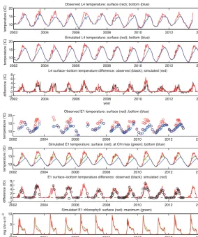
2002 2004 2006 2008 2010 2012 2014 10

15 20

temperature (

ϒ

C)

Observed L4 temperature: surface (red); bottom (blue)

2002 2004 2006 2008 2010 2012 2014

10 15 20

temperature (

ϒ

C)

Simulated L4 temperature: surface (red); bottom (blue)

2002 2004 2006 2008 2010 2012 2014

−2 0 2 4 6 8

year

difference (

ϒ

C)

L4 surface−bottom temperature difference: observed (black); simulated (red)

2002 2004 2006 2008 2010 2012 2014

10 15 20

temperature (

ϒ

C)

Observed E1 temperature: surface (red); bottom (blue)

2002 2004 2006 2008 2010 2012 2014

10 15 20

temperature (

ϒ

C)

Simulated E1 temperature: surface (red); at Chl max (green); bottom (blue)

2002 2004 2006 2008 2010 2012 2014

−2 0 2 4 6 8

difference (

ϒ

C)

E1 surface−bottom temperature difference: observed (black); simulated (red)

20020 2004 2006 2008 2010 2012 2014

5 10

year

mg chl−a m

−3

Simulated E1 chlorophyll: surface (red); maximum (green)

Figure 6. Time series of surface–bottom temperature differences observed and (daily) simulated at L4 and E1 (http://www. westernchannelobservatory.org.uk/data.php).

(see Fig. 1b). When a cold spring is followed by a warm summer (e.g. 2006, 2010, 2013), stratification is particularly strong, with surface–bottom temperature differences reach-ing almost 7◦_{C in the southwest of the region.}

To locally validate the simulation, we use ob-servations at L4 (50◦15.000N, 4◦13.020W) and E1 (50◦02.000N, 4◦22.000W), hydrographic stations that have been occupied weekly and monthly, respec-tively, as part of the Western Channel Observatory (http://www.westernchannelobservatory.org.uk/data.php). Here, seasonal cycles of stratification and phytoplankton dynamics have been extensively studied (Smyth et al., 2010). In Fig. 5, we overplot observed temperature dif-ferences for station occupations within a few days (L4) or 1–2 weeks (E1) of day 190. Observed differences are generally indistinguishable from the simulated differences.

For a more comprehensive validation, Fig. 6 shows time series of surface–bottom temperature differences observed and (daily) simulated at L4 and E1. The temperature at the depth of the maximum chl a concentration is also plotted at E1, confirming the existence of an SCM within the

T day 100 DIN day 100 Chl day 100

Depth (m)

Depth (m)

Depth (m)

Depth (m)

0

-20

-40

-60

15

10

5

0 5 0 10 5 0 10 5 10

0

-20

-40

-60

0

-20

-40

-60 8

4

0

8

4

0

T day 130 DIN day 130 Chl day 130

0

-20

-40

-60

15

10

5

0 5 0 10 5 0 10 5 10

0

-20

-40

-60

0

-20

-40

-60 8

4

0

8

4

0

T day 160 DIN day 160 Chl day 160

0

-20

-40

-60

15

10

5

0 5 0 10 5 0 10 5 10

0

-20

-40

-60

0

-20

-40

-60 8

4

0

8

4

0

T day 190 DIN day 190 Chl day 190

0

-20

-40

-60

15

10

5

0 5 0 10 5 0 10 5 10

0

-20

-40

-60

0

-20

-40

-60 8

4

0

8

4

0

Distance (km) Distance (km) Distance (km)

Figure 7. Sections through the developing tidal mixing front east of Lizard peninsula, along 50.017◦N, on days 100, 130, 160 and 190 of 2013: temperature (left column); dissolved inorganic nitrate (mmol m−3, middle column); chla(mg chlam−3, right column).

the water column is in fact statically stable throughout the time series.

With some confidence in model performance, in Fig. 7 we show temperature, DIN and chlain sections through the de-veloping tidal mixing front east of Lizard peninsula, along 50.017◦_{N, on days 100, 130, 160 and 190 of 2013. We select}

this section as representative of CTD transects undertaken annually in late June/early July by University of Southamp-ton fieldwork students. On day 100 (early April), the water column is well-mixed almost everywhere, with very weak stratification in temperature evident at 10 km along the sec-tion. DIN concentrations are high (∼6 mmol m−3) through-out the water column for bottom depths exceeding a thresh-old value (∼40 m), below which PAR falls below a critical value within the water column. As bottom depths become shallower (progressing inshore), DIN concentrations rapidly fall to near zero, where PAR is sufficient at all depths to sustain plankton growth and associated DIN uptake in the model. Inshore chl a concentrations are accordingly high (12–13 mg chlam−3_{), falling rapidly with distance to} back-ground values (∼0.1 mg chlam−3_)offshore.

By day 130 (early May), the water remains well-mixed, al-though warmer by 1–2◦C, and high productivity has spread offshore, presumably due to intermittent weak stratification during preceding days. By day 160, stratification is clearly established beyond 4 km offshore. DIN concentrations are now reduced to near-zero in the upper 20 m of the strati-fied water, and high chl a concentrations are evidence of

the spring bloom. By day 190, stratification has strength-ened and DIN concentrations in the deep layer of stratified water columns are further depleted through vertical mixing with the upper photic zone, although surface chla concen-trations have by this time substantially declined in the upper layer. The boundary between mixed and stratified waters on days 160 and 190 marks the position of the tidal mixing front. The model has been further used to evaluate the extent of inter-annual variability around the time of annual fieldwork, in the third week of June. Temperature sections on day 169 of 2002–2013 (see Fig. S6) reveal a wide range of offshore stratification and frontal structure in recent years, with the strongest stratification in 2010, the weakest stratification in 2011, and a most clearly defined front in 2009.

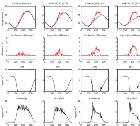
As an example of the seasonal cycles in temperature, sur-face DIN and sursur-face chlaat four locations across the front (spanning the distance range 3–7 m in Fig. S6), Fig. 8 shows evolution of these variables through 2013. Stratification is very marginal and intermittent at 5.033◦W, with surface– bottom temperature differences occasionally reaching 2◦C. DIN concentrations fall close to zero over days 130–300 and chlaconcentrations are high (in the range 6–8 mg chlam−3) throughout this period. Related to the intermittent stratifica-tion are similar fluctuastratifica-tions in chl a. This variability is in part attributed to the near-fortnightly spring–neap tidal cy-cle, which leads to periodic replenishment of nutrients, out of phase with more favourable PAR regimes. Progressing offshore into deeper water, the seasonal cycle transforms towards stronger stratification, a shorter period of surface DIN reduction, and a stronger peak in surface chla around day 150 that corresponds to the spring bloom, followed by substantially lower concentrations during the rest of summer. 3.3 East China and Yellow seas

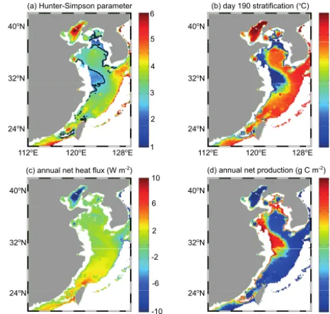
Figure 9 shows example fields for a simulation using the East China Sea and Yellow Sea domain with 2013 forcing. Fig-ure 9a shows the annual-mean Hunter–Simpson parameter, log₁₀(h/u3), which falls below 2.7 in particularly shallow regions (see Fig. 1c) that are also characterized by high am-plitude tidal currents (see Fig. S2); log₁₀(h/u3)conversely exceeds 5.0 in the isolated Bohai Sea, lying to the northwest of the Yellow Sea. As for the northwest European shelf, re-gions with log₁₀(h/u3) <2.7 remain well-mixed throughout summer (Fig. 9b). Elsewhere, stratification is stronger than for the northwest European shelf, with surface–bottom tem-perature differences on day 190 of∼10◦_{C across much of}

the stratified shelf. A major feature of Fig. 9b is the front be-tween mixed and stratified water in the East China Sea that is clearly observed in satellite SST data (Hickox et al., 2000). The simulations also capture the complex system of fronts observed in the Taiwan Strait (Zhu et al., 2013).

0 100 200 300 10

15 20

temperature (

°

C)

5.033°W, 50.017°N

0 100 200 300

−2 0 2 4 6 8

difference (

°

C)

top−bottom difference

0 100 200 300

0 5 10

mmol m

−3

DIN

0 100 200 300

0 5 10

day of year

mg chl m

−3

chlorophyll

0 100 200 300

10 15 20

5.017°W, 50.017°N

0 100 200 300

−2 0 2 4 6 8

top−bottom difference

0 100 200 300

0 5 10

DIN

0 100 200 300

0 5 10

day of year chlorophyll

0 100 200 300

10 15 20

5.000°W, 50.017°N

0 100 200 300

−2 0 2 4 6 8

top−bottom difference

0 100 200 300

0 5 10

DIN

0 100 200 300

0 5 10

day of year

mg chl m

−3

chlorophyll

0 100 200 300

10 15 20

4.983°W, 50.017°N

0 100 200 300

−2 0 2 4 6 8

top−bottom difference

0 100 200 300

0 5 10

DIN

0 100 200 300

0 5 10

day of year chlorophyll

Figure 8. Time series of surface and bottom temperature (red and blue curves), surface–bottom temperature difference, surface DIN and surface chlaconcentrations, across the tidal mixing front east of the Lizard peninsula in 2013.

heat flux field is an important measure of resulting heat imbalances (Fig. 9c). We regard these values as not too excessive, ranging from around 5 W m−2 _{(heat gain) in} the far south to around −10 W m−2 _{(excess heat loss) in} the far north (Bohai Sea). Annual-mean carbon produc-tion rates in the well-mixed shallow regions of the East China Sea range from 300 to 450 g C m−2year−1, falling to∼100 g C m−2year−1in the more extensive stratified re-gion (Fig. 9d). These predictions are similar in magnitude to estimates of primary production based on in situ obser-vations (e.g. 145 g C m−2year−1for “the entire shelf of the East China Sea”, Gong et al., 2003). Monthly mean surface chl a distributions are broadly comparable to satellite ob-servations, although maximum model chl a concentrations are generally double those observed, and the spring bloom is ∼1 month late, in May rather than April (e.g. for 2013, Figs. S7 and S8). Discrepancies between the model and ob-servations in this region may be improved by accounting for higher turbidity in relatively shallow water and model refine-ments related to photo-physiology.

To complete the 3-D picture, Fig. 10 shows show tem-perature, DIN and chl a concentration in sections through the developing front of the central East China Sea, along 32◦N, on days 100, 130, 160 and 190 of 2013. Bottom depth increases considerably with distance offshore. In wa-ter of depth <40 m, the water column remains well-mixed throughout the year, while in deeper water, stratification be-comes established between days 100 and 130. In stratified water, DIN is already depleted in the surface layer over

days 100–130, and is gradually further depleted in the lower layer over days 130–190 through progressive mixing into the photic zone. A local surface maximum in chlaconcentration is evident at the frontal boundary (∼250 km) on day 130, while a SCM is evident in stratified water on days 160 and 190. The SCM is most clearly defined at∼25 m on day 190.

4 Summary and discussion

We have developed S2P3-R, a versatile framework for effi-cient modelling of physical and biological phenomena and processes in shelf seas, adopting an existing 1-D model, S2P3. Here, we complement ongoing development and use of the 1-D model for specific research hypotheses (e.g. Bauer and Waniek, 2013) and in educational settings, where ideal-ized simulations (e.g. Sharples, 2008) are linked to realis-tic situations such as fieldwork contexts – e.g. off Cornwall, away from the lateral influences of runoff.

(d) annual net production (g C m-2₎

(c) annual net heat flux (W m-2₎

(a) Hunter-Simpson parameter (b) day 190 stratification (o_C)

40o_N

32o_N

24o_N

112o_{E 120}o_{E 128}o_E

6

3

1 2 4 5

40o_N

32o_N

24o_N

112o_{E 120}o_{E 128}o_E

12

4

1 2 6 8

40o_N

32o_N

24o_N

112o_{E 120}o_{E 128}o_E

450

150

50 250 350

40o_N

32o_N

24o_N

112o_{E 120}o_{E 128}o_E

10

-2

-10 -6 2 6

10

Figure 9. For the East China and Yellow seas domain in 2013: (a) Hunter–Simpson parameter, highlighting the contour delineating log₁₀(h/u3)=2.7; (b) day 190 surface–bottom temperature difference; (c) net surface heat flux; (d) annual net production.

L4/E1) can be compared with indirect estimates computed from time-integrated heat fluxes, winds and tidal currents at the same locations. If local heat fluxes and tidal/wind mix-ing dominate the annual cycle of stratification, directly cal-culated and indirectly estimated time series of PEA tendency should be similar.

Where appropriate, the framework facilitates experiments to investigate the sensitivity of measurable quantities (e.g. chlaconcentration) to a wide range of physical and biologi-cal processes that can be adjusted with corresponding model parameters. Where high-quality observations are available (e.g. at E1 in the western English Channel), S2P3-R thus pro-vides a means for improving our fundamental understanding of the system. With tuned parameters, S2P3-R furthermore provides the means to carry out credible multi-year simula-tions of physical and biological processes and property dis-tributions at appropriately high temporal, vertical and hori-zontal resolution.

At the seasonal timescale, the most striking surface fea-tures are TMFs. Realistic representation of TMFs, demand-ing high horizontal resolution, amounts to first-order eval-uation of any simulation, e.g. the UK Met Office forecast system (O’Dea et al., 2012), which has the same relatively coarse (12 km) resolution as our northwest European shelf domain. The summer surface–bottom temperature differ-ences across the northwest European shelf and the associ-ated TMFs in S2P3-R (Fig. 3a) compare well with the 3-D model results (O’Dea et al., 2012, their Fig. 10). Our simpler approach thus indicates the importance of 1-D processes in

forming these features, the locations of which are consistent with these more complex models.

It is natural to deploy S2P3 across multiple processors, with sub-domains computed independently in parallel. This has been trialled for twelve 1◦×1◦sub-domains across the southern Celtic Sea and western English Channel at a reso-lution of 1 km, substantially expanding our western English Channel domain with essentially no extra computational ex-pense. Figure 11 shows the July surface–bed temperature dif-ference across this region, illustrating how we are able to effi-ciently simulate regional stratification at very high horizontal resolution.

We have evaluated the model in various ways with available observations, specifically addressing spatial pat-terns, vertical structures, and seasonal–interannual variabil-ity. Temperature distributions are reproduced with consider-able success, as are key aspects of the spatial and temporal variability in nutrient and chlaconcentrations. In particular, we are able to accurately reproduce monthly observations of thermal structure at station E1 in the western English Chan-nel over 2002–2013 (Fig. 6), providing confidence in the use of S2P3-R in this region. We therefore consider there is much potential for S2P3-R to investigate physical and physiologi-cal controls on primary productivity at regional sphysiologi-cales.

T day 100 DIN day 100 Chl day 100

Depth (m)

24

18

12

0 500 0 0

8

4

0

8

4

0

T day 130 DIN day 130 Chl day 130

0 0 0 8

4

0

8

4

0

T day 160 DIN day 160 Chl day 160

0 0 0 8

4

0

8

4

0

T day 190 DIN day 190 Chl day 190

0 0 0 8

4

0

8

4

0

Distance (km) Distance (km) Distance (km)

Depth (m)

Depth (m)

Depth (m)

500 500

500 500 500

500 500 500

500 500 500

24

18

12

24

18

12

24

18

12 0 -50

-100

-150

0 -50

-100

-150

0 -50

-100

-150

0 -50

-100

-150 0

-50

-100

-150

0 -50

-100

-150

0 -50

-100

-150

0 -50

-100

-150

0 -50

-100

-150

0 -50

-100

-150

0 -50

-100

-150

0 -50

-100

-150

Figure 10. Sections through the developing tidal mixing front of the East China Sea, along 32◦N, on days 100, 130, 160 and 190 of 2013: temperature (left column); DIN (mmol m−3, middle column); chla(mg chlam−3, right column).

– The coastal zone around Cornwall, typified by station L4, is strongly influenced by riverine inputs that pro-mote surface freshening and stratification and alter light attenuation by non-algal particles and dissolved organic matter (Groom et al., 2009; Smyth et al., 2010). – The northern North Sea is strongly influenced by shelf

edge exchange that leads to the inflow of relatively warm and salty Atlantic Water (Huthnance et al., 2009). – The Yangtze River and two branches of the Kuro Shio – the Taiwan current and the Tsushima warm current – exert strong influences on stratification and productivity in the East China Sea (e.g. Son et al., 2006).

Further development of S2P3-R will formally establish the (presently prototype) option to prescribe spatially variable initial temperatures and meteorological variables, interpo-lated appropriately to each model mesh. As an additional diagnostic, the thermal wind balance may be used with the simulated density field to infer the residual flows that are as-sociated with TMFs (e.g. Hill et al., 2008), indicating the po-tential importance of net advection along the fronts.

In summary, the S2P3-R framework (v1.0) provides the flexibility to undertake research experiments in finely re-solved realistic domains where 1-D processes dominate, to test hypotheses regarding the sensitivity of 1-D biogeochem-ical processes to key model parameters, and/or to test the re-sponses to variations of physical forcing on timescales rang-ing from diurnal to inter-annual. Combinrang-ing flexibility with

Figure 11. Surface–bottom temperature differences (◦C) across the southern Celtic Sea and western English Channel, in mid-July of 2014, simulated with S2P3-R configured in twelve 1◦×1◦ sub-domains, as indicated.

computational efficiency, the S2P3-R framework may fur-ther contribute to capacity building in marine monitoring and management for individuals/organisations without the resources to run or analyse complex models of their terri-torial waters or exclusive economic zones.

Code availability

The S2P3-R (v1.0) framework, comprising source code along with example scripts and output, is available online from ftp://ftp.noc.soton.ac.uk/pub/rma/s2p3-reg.tar.gz.

Unzipped and uncompressed, the directory/s2p3_reg_v1 contains several sub-directories:

– /main contains the source code, s2p3v7_reg_v1.f90, which is compiled “stand alone”, and executed us-ing accompanyus-ing scripts, with examples of “map” (the northwest European Shelf simulation, as Fig. 3), “section” (Celtic Sea) and “time series” (E1) simula-tions (run_map, run_section and run_timeseries, respec-tively).

– /domain contains bathymetry and tide data for the northwest European Shelf region (s12_m2_s2_n2_h_map.asc), for a selected north–south section in the Celtic Sea (s12_m2_s2_n2_h_sec.asc) and for a selected point, E1 in the western English Channel (s12_m2_s2_n2_h_tim.asc).

– /met contains climatological meteorological forcing (Celtic_met.dat).

– /output contains example output data from the three runs (map, section, time series).

– /plotting contains MATLAB scripts for plotting maps, sections and time series (plot_map, plot_section and plot_timeseries, respectively).

The Supplement related to this article is available online at doi:10.5194/gmd-8-3163-2015-supplement.

Acknowledgements. Jeff Blundell assisted with initial editing of the S2P3 source code. Ivan Haigh ran the OSU Tidal Prediction Software to predict tidal current amplitudes in the East China and Yellow seas. Data at L4 and E1 were downloaded from http://www.westernchannelobservatory.org.uk/data with thanks to the Western Channel Observatory community. R. Marsh acknowledges the support of a 2013 Research Bursary awarded by the Scottish Association for Marine Science. A. E. Hickman was partly funded by a Natural Environment Research Council fellowship (NE/H015930/2). We thank three anonymous reviewers for a series of insightful comments that helped us to focus the paper.

Edited by: A. Yool

References

Amante, C. and Eakins, B. W.: ETOPO1 1 Arc-Minute Global Relief Model: Procedures, Data Sources and Analysis. NOAA Technical Memorandum NESDIS NGDC-24, 19 pp., 2009. Bauer, A. and Waniek, J. J.: Factors affecting the chlorophyll a

con-centration in the central Beibu Gulf, South China Sea, Mar. Ecol. Prog. Ser., 474, 67–88, doi:10.3354/meps10075, 2013.

Edwards, K. P., Barciela, R., and Butenschön, M.: Validation of the NEMO-ERSEM operational ecosystem model for the North West European Continental Shelf, Ocean Sci., 8, 983–1000, doi:10.5194/os-8-983-2012, 2012.

Egbert, G. D. and Erofeeva, S. Y.: Efficient Inverse Modeling of Barotropic Ocean Tides, J. Atmos. Ocean. Tech., 19, 183–204, doi:10.1175/1520-0426(2002)019<0183:EIMOBO>2.0.CO;2, 2002.

Egbert, G. D., Bennett, A. F., and Foreman, M. G. G.:

TOPEX/POSEIDON tides estimated using a global

inverse model, J. Geophys. Res., 99, 24821–24852,

doi:10.1029/94JC01894, 1994.

Geider, R. J., MacIntyre, H. L., and Kana, T. M.: A dynamic model of phytoplankton growth and acclimation: responses of the balanced growth rate and chlorophylla: carbon ratio to light, nutrient-limitation and temperature, Mar. Ecol. Prog. Ser., 148, 187–200, 1997.

Gong, G.-C., Wen, Y.-H., Wang, B.-W., and Liu, G.-J.: Seasonal variation of chlorophyll a concentration, primary production and environmental conditions in the subtropical East China Sea, Deep-Sea Res. Pt. II, 50, 1219–1236, 2003.

Groom, S., Martinez-Vicente, V., Fishwick, J., Tilstone, G., Moore, G., Smyth, T., and Harbour, D.: The Western English Chan-nel Observatory: optical characteristics of station L4, J. Marine Syst., 77, 278–295, 2009.

Hickman, A. E., Holligan, P. M., Moore, C. M., Sharples, J., Krivtsov, V., and Palmer, M. R.: Distribution and chromatic adap-tation of phytoplankton within a shelf sea thermocline, Limnol. Oceanogr., 54, 525–536, 2009.

Hickman, A. E., Moore, C. M., Sharples, J., Lucas, M. I., Tilstone, G. H., Krivtsov, V., and Holligan, P. M.: Primary production and nitrate uptake within the seasonal thermocline of a stratified shelf sea, Mar. Ecol. Prog. Ser., 463, 39–57, doi:10.3354/meps09836, 2012.

Hickox, R., Belkin, I., Cornillon, P., and Shan, Z.: Climatology and Seasonal Variability of Ocean Fronts in the East China, Yellow and Bohai Seas from Satellite SST Data, Geophy. Res. Lett., 27, 2945–2948, 2000.

Hill, A. E., James, I. D., Linden, P. F., Matthews, J. P., Prandle, D., Simpson, J. H., Gmitrowicz, E. M., Smeed, D. A., Lwiza, K. M. M., Durazo, R., Fox, A. D., and Bowers, D. G.: Dynamics of tidal mixing fronts in the North Sea [and discussion], Philos. T. R. Soc. Lond., 343, 431–446, 1993.

Hill, A. E., Brown, J., Fernand, L., Holt, J., Horsburgh, K. J., Proctor, R., Raine, R., and Turrell, W. R.: Thermohaline circu-lation of shallow tidal seas, Geophys. Res. Lett., 35, L11605, doi:10.1029/2008GL033459, 2008.

Holligan, P. M., Williams, P. J. L., Purdie, D., and Harris, R. P.: Photosynthesis, respiration and nitrogen supply of plankton pop-ulations in stratified, frontal and tidally mixed shelf waters, Mar. Ecol. Prog. Ser., 17, 201–213, 1984.

Holt, J., Harle, J., Proctor, R., Michel, S., Ashworth, M., Batstone, C., Allen, I., Holmes, R., Smyth, T., Haines, K., Bretherton, D., and Smith, G.: Modelling the global coastal ocean, Philos. T. R. Soc. A, 367, 939–951, doi:10.1098/rsta.2008.0210, 2009a. Holt, J., Wakelin, S., and Huthnance, J.: Down-welling circulation

of the northwest European continental shelf: A driving mecha-nism for the continental shelf carbon pump, Geophys. Res. Lett., 36, L14602, doi:10.1029/2009GL038997, 2009b.

Huthnance, J. M., Holt, J. T., and Wakelin, S. L.: Deep ocean ex-change with west-European shelf seas, Ocean Sci., 5, 621–634, doi:10.5194/os-5-621-2009, 2009.

Joint, I. and Groom, S. B.: Estimation of phytoplankton production from space: current status and future potential of satellite remote sensing, J. Exp. Mar. Biol. Ecol., 250, 233–255, 2000.

Joint, I., Wollast, R., Chou, L., Batten, S., Elskens, M., Edwards, E., Hirst, A., Burkill, P., Groom, S., Gibb, S., Miller, A., Hy-des, D., Dehairs, F., Antia, A., Barlow, R., Rees, A., Pomroy, A., Brockmann, U., Cummings, D., Lampitt, R., Loijens, M., Mantoura, F., Miller, P., Raabe, T., Alvarez-Salgado, X., Stelfox, C., and Woolfenden, J.,: Pelagic production at the Celtic Sea shelf break, Deep-Sea Res., 48, 3049–3081, doi:10.1016/S0967-0645(01)00032-7, 2001.

Kalnay, E., Kanamitsu, M., and Kistler, R.: The NCEP/NCAR 40-year reanalysis project, B. Am. Meteor. Soc., 77, 437–470, 1996. Moore, C. M., Suggett, D., Holligan, P. M., Sharples, J., Abraham, E. R., Lucas, M. I., Rippeth, T. P., Fisher, N. R., Simpson, J. H., and Hydes, D. J.: Physical controls on phytoplankton physiology and production at a shelf sea front: a fast repetition-rate fluorom-eter based field study, Mar. Ecol. Prog. Ser., 259, 29–45, 2003. Moore, C. M., Suggett, D. J., Hickman, A. E., Kim, Y. N.,

Twed-dle, J. F., Sharples, J., Geider, R. J., and Holligan, P. M.: Phy-toplankton photoacclimation and photoadaptation in response to environmental gradients in a shelf sea, Limnol. Oceanogr., 51, 936–949, 2006.

NEMO and SST data assimilation for the tidally driven European North-West shelf, Journal of Operational Oceanography, 5, 3–17, 2012.

Pemberton, K., Rees, A. P., Miller, P. I., Raine, R., and Joint, I.: The influence of water body characteristics on phytoplankton di-versity and production in the Celtic Sea, Cont. Shelf Res., 24, 2011–2028, 2004.

Pingree, R., Holligan, P., and Mardell, G. T.: The effects of verti-cal stability on phytoplankton distributions in the summer on the northwest European Shelf, Deep Sea Res., 25, 1011–1028, 1978. Rees, A. P., Joint, I., and Donald, K. M.: Early spring bloom phytoplankton-nutrient dynamics at the Celtic Sea Shelf Edge, Deep-Sea Res. Pt. II, 46, 483–510, 1999.

Sharples, J.: Investigating the seasonal vertical structure of phyto-plankton in shelf seas, Marine Models Online, 1, 3–38, 1999. Sharples, J.: Potential impacts of the spring-neap tidal cycle on shelf

sea primary production, J. Plankton Res., 30, 183–197, 2008. Sharples, J., Ross, O. N., Scott, B. E., Greenstreet, S., and Fraser,

H.: Inter-annual variability in the timing of stratification and the spring bloom in the North-western North Sea, Cont. Shelf Res., 26, 733–751, 2006.

Sharples, J., Tweddle, J. F., Green, J. A. M., Palmer, M. R., Kim, Y.-N., Hickman, A. E., Holligan, P. M., Moore, C. M., Rippeth, T. P., Simpson, J. H., and Krivtsov, V.: Spring-neap modulation of internal tide mixing and vertical nitrate fluxes at a shelf edge in summer, Limnol. Oceanogr., 52, 1735–1747, 2007.

Simpson, J. H. and Bowers, D. G.: Geographical variations in the seasonal heating cycle in northwest European shelf seas, Annales Geophysicae, 2, 411–416, 1984.

Simpson, J. H. and Hunter, J. R.: Fronts in the Irish Sea, Nature, 250, 404–406, 1974.

Simpson, J. H. and Sharples, J.: Introduction to the Physical and Biological Oceanography of Shelf Seas, Cambridge University Press, Cambridge, UK, 2012.

Smyth, T. J., Fishwick, J. R., Al-Moosawi, L., Cummings, D. G., Harris, C., Kitidis, V., Rees, A., Martinez-Vicente, V., and Wood-ward, E. M. S.: A broad spatio-temporal view of the Western English Channel observatory, J. Plankton Res., 32, 585–601, doi:10.1093/plankt/fbp128, 2010.

Son, S., Yoo, S., and Noh, J.-H.: Spring phytoplankton bloom in the fronts of the East China Sea, Ocean Sci. J., 41, 181–189. doi:10.1007/BF03022423, 2006.

Weston, K., Fernand, L., Mills, D., Delahunty, R., and Brown, J.: Primary production in the deep chlorophyll maximum of the cen-tral North Sea, J. Plankton Res., 27, 909–922, 2005.