Evaluation of SURM and GR4J rainfall runoff models, for the Nazloo River catchment in northwest of Iran

World Journal of Environmental Biosciences

All Rights Reserved WJES © 2014

Available Online at:

www.environmentaljournals.org

Volume 5, Issue 2: 26-34

ISSN 2277- 8047

Evaluation of SURM and GR4J rainfall runoff models, for the Nazloo River catchment in

northwest of Iran

Hossein Rezaie

_{, Anahita Jabbari}

_{, Javad Behmanesh}

_{, Ben Jarihani}

_{and Behzad}

Hessari

1

Associate professor in Department of Water Engineering, Urmia University, Urmia, Iran

2

_{PhD candidate of water engineering, Urmia University, Urmia, Iran}

3

Associate professor in Department of Water Engineering, Urmia University, Urmia, Iran

4

Post-doctoral Research fellow, University of the Sunshine Coast, Queensland, Australia

5

Assistant professor in Department of Water Engineering, Urmia University, Urmia, Iran

____________________________________________________________________________________________________________________________________________________________________

ABSTRACT

The right hydrological model selection is an important task in today’s hectic race of developing powers of modelling platforms. In this regard, there is a newly developed modelling system which meets all needs of Integrated Water Resources Management practices, under a same modelling platform which nowadays is a very important lost part of the management cycle. Source Integrated Modelling System (IMS)as a very comprehensive product of CRCCH (Cooperative Research Center for Catchment Hydrology)Australia is a new attempt in order to model the whole catchment procedures in one platform. In the current study the two of most well-known rainfall runoff (RR) models from modelling component of the Source have been selected in order to compare their application and the possibility of applying Source package in the different climate from Australia. The GR4J and SURM models have been studied by daily input data, and results showed that the GR4J model with a NSE (Nash-Sutcliffe Efficiency) amount about 0.62 represents a better simulation of the catchment. At the same time the survey form was designed and sent to hydrological modelers in order to ask some of the most challenging RR modelling problems. The results illustrated that the NSE coefficient is the most popular efficiency criterion for modelling practices and choosing the GR4J model parameter sets as preferred parameters is in agreement with survey form results to. The overall outcome is that the Source platform can be applied for other climates than Australia as well.

Key words: Source integrated Modelling System –Rainfall Runoff Modelling– Urmia Lake basin – Survey Form

____________________________________________________________________________________________________________________________________________________________________ Corresponding author: Anahita Jabbari

e-mail _{[email protected]}

Received: 12 September 2016 Accepted: 16 December 2016

INTRODUCTION

Today, hydrological models have become widely used for gaining the proper solutions for various aquatic and environmental problems of catchments. The computational rainfall runoff (RR) models have the most application in hydrological practices and are the most crucial part of the water resources management procedure. Along with the rapid growth of the computing capabilities and modelling powers, and availability of new data sources such as remote sensing, the choose of appropriate model has become important task to produce the acceptable output by minimum data requirement and in lower time. Nearly 150 years ago the first widely used RR model was developed by the Irish engineer Thomas James Mulvaney which was named rational method(Beven 2011), but Stanford catchment model (SWM) is the first attempt for numerical modelling of the catchments(Crawford 1966). Ever since then, a rapid improvement has occurred in developing catchment models. Today there are numerous models that can be used to address similar problem in a catchment. However the right model selection became the hot topic of modelling practices especially in data sparse environments. This decision is even more difficult under the different circumstances of modelling practices, as a result nowadays one of the most important factors in managing the water systems is the ability to gather all of the management tools in one platform. Along with the growing need to identify similar modelling bases, As a very new modelling platform, eWater Source, the Australia’s national hydrological modelling platform is presented to address lots of water management

problems. Source Integrated Modelling System (IMS) gathers the all required components of catchment water resources management in one frame. It includes three modes (catchment runoff, river management and river operations) for different applications which have been presented in a very new researches (Dutta, Wilson et al. 2013, Rassam, Peeters et al. 2013, Hughes, Dutta et al. 2014, Peeters, Podger et al. 2014, Podger, Cuddy et al. 2014, Turner, Marlow et al. 2014). The catchment component of the Source system contains some of the most famous conceptual rainfall runoff models (Delgado 2013). There are eleven choices of runoff generation options in Source, in order to simulate RR processes. This is one of the most important advantages of Source that run multiple models in the same platform.

Anahita Jabbari

et al

World J Environ Biosci, 2016, 5, 2: 26-34

MATERIALS AND METHODS

Nazloo River Basin

Figure 1: Nazloo River catchment and Urmia Lake

Urmia Lake

Study site and data sets

The study site is in the Urmia Lake Basin (ULB) one of the most important water bodies in the area and the second largest salt lake in the world. Due to its important Eco hydrologicrole in the north-west of Iran, it was always considered as a significant hydrologic component at the region. Due to water management problems, surface water over uses (especially in agriculture sector), the balance of input and output of the lake has been disturbed. The ULB is an internally draining catchment with two main water inputs, river discharge and direct rainfall on the lake surface. The mean annual volume of all the water input to the lake basin is about 17 Billion cubic meters which about 10.8 Billion cubic meters of it returns to atmosphere due the evaporation. So the remaining volume about 6.2 Billion cubic meters is the whole available water at the current circumstances. All above mentioned factors causes the shrinkage of the lake level most rapidly at the recent 10 years. The ecologic water level of the lake is 1274.1 m and the maximum observed level was 1278.41 m in the historic period from 1967.

Figure 2: The structure of SURM model (CRCCH 2010)

Forecasting inflow to Urmia Lakefrom its sub catchments is crucial to understanding the lake’_{s upcoming condition and to} take right management decisions on the base of the accurate knowledge in time. Choosing right model with respect to data availability which can accurately reflect the spatial and temporal behavior of the catchment has a significant role in transforming modelling process from a hydrological practice to applicable decision making supporters. After becoming an environmental change hotspot in recent years by United Nations Environmental Program (UNEP, 2015), there have been number of modeling practices from any type, targeting Urmia Lake basin and its catchments, mainly without considering the data availability and model complexities. The combination of all above depletions with the misunderstood issue of “a more complex models leads to more accurate results” might result in incorrect modelling practices. There is also an arbitrary interpretation of the model evaluation statistics that worsen the mentioned problems, therefore the survey questionnaire has been designed and sent to professional rainfall runoff modelers in order to gain more reliable ranges for model evaluation parameters such as Nash coefficient. Although there has been some few studies took place in the survey form (Chiew and McMahon 1993) but the current study just focus on daily rainfall runoff modeling evaluation parameters. Therefore the objectives of this study are

i) to adopt new Source integrated modeling platform which was developed by eWater Australia to Lake Urmia catchment conditions; ii) to choose best modelling practices with respect to data availability and model complexity; and iii) to compare two selected parsimonious rainfall runoff models in simulating hydrological processes of Nazloo River.

There are 15 rivers which reach to the lake and the Nazloo River is one of them at the west side of the lake. This catchment is located at 44° 24´ and 45° 53´ longitudes and 37° 30´ and 37° 58´ latitudes. The maximum and minimum elevations of the catchment are 1291 m and 3600 m, respectively. This river is one of the main rivers draining into the ULB (Fig. 1). The total area of the catchment is about 2020 km2 _{which the area about 505} km2 _{of it is located in Turkey, that are mountainous regions} with the most snow fall and the least available climate measured data(Hessari 2010). The catchment outlet is at the Abajaloo hydrometery station with the elevation of 1290 m. The upstream basin is the most agricultural land use dominant region in all over the catchment. Indeed the most agricultural activities take place between Tapik (where the head flow to the Abajaloo sub basin is measured), located about 1400 m above the sea level, and Abajaloo stations. Figure 1 illustrates the case study catchment and its condition on the map.

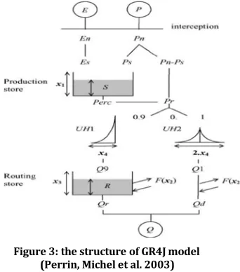
Figure 3: the structure of GR4J model (Perrin, Michel et al. 2003)

Anahita Jabbari

et al

World J Environ Biosci, 2016, 5, 2: 26-34

considering corrective coefficients. The daily evapotranspiration was calculated from evaporation data as well.

Model description

Source integrated modelling system and its catchment runoff component

For the current study case although it is better to use distributed physically based models but in the aspect of available data in the region we need the conceptual models platform like the one eWater has been developed. Source IMS has a capability to relate several components of catchments using a comprehensive node- link net. It allows users to understand the complex relationships between catchment elements in a much more simple way. The integration of multiple modules in one package is another advantage of Source. The components of source are as follows (Welsh, Vaze et al. 2013):i) catchment runoff; ii) river system network; iii) interactions between surface water with groundwater system; iv) water quality; v) river regulation and storages; vi) urban, irrigation and environmental demands; and vii) complex river management rules.

This system added the benefits of digital elevation model (DEM) to the comprehensive node-link network in order to have more detailed view of the scenarios. Adding DEM to the software enables the user to define different models for each sub catchment or functional units. For example if it is previously identified that the forested areas of a sample catchment confirm with Australian Water Balance Model (AWBM), it is possible to define it for those parts and run a model with different RR models for other sub catchments. This is the main advantage of applying DEM in Source. The basic temporal scale for rainfall runoff models are daily but the monthly time steps may be applied to. There is no limitation on the catchment size, Source can be used on large catchments and even so small catchments like the catchments are modeled with SURM, which is basically the urban RR modeling system. All available rainfall runoff models in Source are conceptual models as follows: AWBM (Boughton 2004), IHACRES (Croke, Andrews et al. 2006),while the pc IHACRES version 1 was developed by collaboration between institute of hydrology United Kingdom and the Australian National University, Canberra (Jakeman, Littlewood et al. 1990, Littlewood, Down et al. 1997), Sacramento (Burnash 1973), SIMHYD (Chiew and McMahon 2002, Chiew 2002), SMARG(Goswami, O’Connor et al. 2002, Vaze, Barnett et al. 2004), GR4J (Perrin, Michel et al. 2003), and SURM (developed by CRC catchment hydrology as the base model for MUSIC)(Delgado 2013, eWater 2013).The aforementioned methods generate the stream flow with a suitable model. The other two flow generation options available in the catchment component of Source are as follows: Nil runoff, which makes no flow generation or observed catchment runoff depth and observed catchment surface runoff depth which the first one considers observed depth of time series for runoff and uses a digital filter to separate the quick flow and slow flow components and the last one assumes that all runoff in the time series is surface flow, and so quick flow is set equal to the observed flow, and slow flow is set to zero(Grayson 1996). All of the models can be applied for sub catchments separately or for whole catchment. Though all these models have been applied widely in numerous studies(Littlewood, Down et al. 1997, Post and Jakeman 1999, Peel, Chiew et al. 2000, Chiew and McMahon 2002, Goswami, O’Connor et al. 2002, Tuteja, Beale et al. 2003, Boughton 2004, Gan and Burges 2006, Tuteja, Vaze et al. 2007, Simonneaux, Hanich et al. 2008, Chiew 2010, Harlan, Wangsadipura et al. 2010, Vaze, Post et al. 2010, Basri 2013), there are many reports on the RR model selection, and their application in different criterion of data availability, model complexity and model performance (eWater 2005a, eWater 2005b).Source IMS provides the users with the wide range of RR models, from simple with low parameters number up to more complex models. Here we used the GR4J, one of the most applied conceptual and simple models (Perrin, Michel et al. 2003, Simonneaux, Hanich et al. 2008, Harlan, Wangsadipura et al. 2010, Vaze 2012), and SURM, as a simplified version of SimHyd model. GR4J and SURM models both are daily, conceptual rainfall runoff models which belong to the

family of explicit soil moisture accounting models (ESMA), varied in the number of storage elements used, the functions controlling the exchanges, and consequently in the number and type of parameters required (O’Connell 1991). So the all differences between these models related to the selected model factors that make them more complex or simple to use. As a result there is no separation between the rainfalls that is occurred on pervious or impervious surfaces. The model then goes through the series of two vertically located stores and calculates the equations of model. Originally the model had four parameters of X1, X2, X3, and X4. However in Source the GR4J includes six parameters, all four parameters above plus additional C and K parameters. These two parameters are used to separate the base flow and quick flow in output results without any changes in model simulation results. Using these two parameters are optional and leaving them in their default values as zero will terminates this operation of model, and all runoff will be proposed as quick flow.

Table 2 illustrates the GR4J model parameters, and their descriptions. The detailed processes of the model and its equations are presented elsewhere (Perrin and Littlewood 2000, Perrin, Michel et al. 2003).

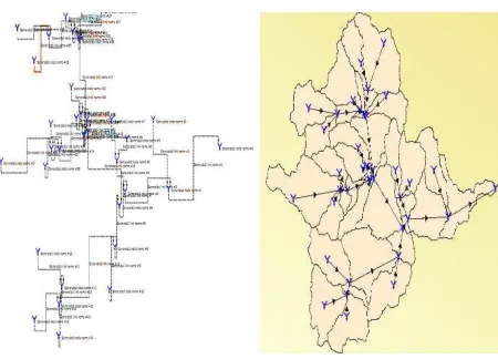
Figure 4: the shematic and geographic scenarios of Nazloo RiverCatchment

Model setup

Source supports two types of model setup: geographic and schematic. In order to model the RR processes of a catchment, the catchment is defined through geographic scenario by following a step by step procedure. First, the catchment DEM is loaded to the geographic scenario definition space. Source itself can extract the river network system by identifying the number of sub catchments which is an optional choice by the user. The river network density is identified by the minimum catchment size which is an optional choice, the smaller the sub catchment size, denser the river network. Next, the catchment outlet is chosen either by the shape file of the GIS or automatic selection via Source. The functional unit’s selection enables the user to define a variety of RR models for each for example land use unit. At the end of this step the node-link system is generated and the relation between sub catchments and the water transmitting links are defined. Figure 4 shows the geographic and schematic representation of the Nazloo River catchment.

Anahita Jabbari

et al

World J Environ Biosci, 2016, 5, 2: 26-34

each of them. The SURM model which is the default model for MUSIC package by CRC catchment hydrology and GR4J catchment model which was used numerous times in successful researches although it’s simple structure (eWater 2013).

Calibration analysis is the next step in RR modelling. The observed daily runoff data in order to calibrate the models is loaded at this stage. The data is collected from Abajaloo station at the outlet of the Nazloo River, after the main agricultural water use in the catchment and right before the lake estuary (Figure 1). This station is the last station which the entire catchment water yield crosses from that point and there are no noticeable agricultural activities after that point. So the recorded runoff represents all water yield of the catchment reaches to the lake.

The other advantage of Source system is definition of Meta parameters which enables the user to group the parameters with the same changing domain in order to run the calibration stage more easily. The possibility of auto grouping the parameters for producing Meta parameters is another facility of the package. All same named parameters were defined as Meta parameters because the selected models were applied for the entire of catchment regardless of functional units or catchments.

So in calibration stage the models are calibrated by the use of different objective functions and optimization methods. The results of calibrated method are the reported numbers of Meta parameters and the table of all calibrated parameters of each calibration. The simulation is then applied at the last stage by using the best parameter set which is identified by objective functions. Source provides lots of facilities to represent output data, such as tables, figures and statistical properties of observed and simulated flows.

Efficiency assessment and survey form

Source provides four optimization method options plus manual optimization possibility, as follows: Shuffled Complex Evolution (SCE), Uniform Random Sampling, Rosenbrock and SCE-then- Rosenbrock. As a global widely used method, we chose SCE in current study which has been widely used and tested in other studies (Wu and Zhu 2006, Goswami and O'CONNOR 2007, Muttil and Jayawardena 2008, Seong, Her et al. 2015, Zhang, Wang et al. 2015). SCE (Duan, Sorooshian et al. 1992, Duan, Gupta et al. 1993, Duan, Sorooshian et al. 1994) is the most widely used optimization method for calibrating catchment models in recent years (Shoemaker, Regis et al. 2007).

Moreover, several objective functions which may be selected by the modeler in calibration stage, are available in Source.The combination of all objective elements produces seven objective functions choices as follows: Nash-Sutcliffe Efficiency (NSE) Daily, NSE Monthly, NSE Monthly and Bias Penalty, NSE Daily and Flow Duration, NSE Daily and log Flow Duration, Minimize Absolute Bias, NSE Daily and Bias Penalty. There is also a possibility to identify the weighting of NSE coefficient in combined objectives. The NSE(Nash and Sutcliffe 1970)is a model evaluation coefficient that extensively used in all hydrological (and other) modelling studies (Krause, Boyle et al. 2005, Moriasi, Arnold et al. 2007, Chiew, Teng et al. 2009, Vaze 2012). The Nash- Sutcliffe efficiency is a normalized statistic that determines the relative magnitude of the residual variance (“noise”) compared to the measured data variance (“information”) (Nash and Sutcliffe 1970). It is the indicator of how simulated data fits with observed data and ranges from -∞ to +1 which +1 shows the perfect fitness. So the closer amounts of Nash to +1, the better estimation of stream flow and model performance. Due to its lots of applies in previous studies, it is used here to. Moreover it is suggested by ASCE to (ASCE 1993).

There are a few but important studies on acceptable range of NSE values in RR modeling practices to address the best parameters set. This is important to know the sufficient amount of each efficiency coefficient in order to choose the best model. Chiew and McMahon (1993), based on a survey of 63 professional hydrologists, for monthly runoff simulations indicated that the NSE monthly values of 0.6 or more are “generally satisfactory”

while another study(Yu and Zhu 2014) adopted their reported ranges for daily simulations They have found that NSE values over 0.7 show acceptable performance for daily simulations.

As an experiment, in the current study we developed a survey questionnaire and asked hydrological modelers what is the main challenges in daily rainfall runoff modelling. Moreover the issues of model complexity, data availability and model performance were asked as modelling common challenges. We specifically asked the acceptable NSE values for daily RR simulations. The results showed 70% agreement among hydrologists on NSE daily values over 0.6 in order to have the best model performance. However, in order to have acceptable model performance minimum 0.5 for NSE is required. Among 12 widely used questioned objective functions, NSE was the first favorite coefficient with 47% of all votes.

RESULTS

SURM model

Although the Source integrated system was first developed to meet the needs of Australian water management problems, but this is an advisable system for other catchment systems. The two models were both calibrated through outlet generated node at Abajaloo station. The one year warm up period was considered for both models up to 23 September 1998. The best parameter set in calibration process for SURM model resulted the NSE amount of 0.4 which was the maximum daily coefficient under the same model run conditions with GR4J model. The Figure 5 represents the observed vs simulateddischarges from SURM model.

GR4J model

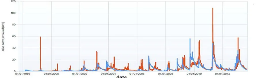
The calibration results for best calibrated model in GR4J model is illustrated by the 0.62 as the best amount for NSE daily objective function. The optimization method which was used is Shuffled Complex Evolution. Figure 6 shows the comparison between observed and simulated discharges. The best parameters set with NSE daily objective function were recorded as follows: X1= 397.856, X2= 3.271, X3= 20.033, X4= 1.481, C= 0.443 and K= 0.783. Approximately all the parameters are in 80% confidence interval except the X2 moderate bias from the upper range of the 80% interval.

DISCUSSION

As it mentioned before, the SURM model is originally anRR model for urban areas(CRCCH 2010). The Nazloo Rivercatchment is a combination of urban and agricultural and other land uses, so the weaker performance of SURM in comparison with GR4J may be described in this way.

Anahita Jabbari

et al

World J Environ Biosci, 2016, 5, 2: 26-34

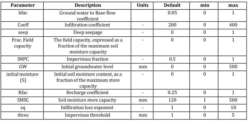
Table 1: The parameters definition of the SURM model

Parameter Description Units Default min max

bfac Ground water to Base flow

coefficient 0.05 0 1

Coeff Infiltration coefficient - 200 0 400

seep Deep seepage - 0 0 1

Frac. Field

capacity The field capacity, expressed as a fraction of the maximum soil moisture capacity

- 0 0 1

IMPC Impervious fraction - 0.5 0 1

GW Initial groundwater level mm 0 0 500

initial moisture

(S) Initial soil moisture content, as a fraction of the maximum store capacity

- 0 0 1

Rfac Recharge coefficient - 0.25 0 1

SMSC Soil moisture store capacity mm 120 1 500

sq Infiltration loss exponent - 1 0 10

thres Impervious threshold mm 1 0 5

Table 2: the parameters of GR4J model

parameter description units median

value confidence 80% interval

min max

X1 maximum capacity of

production store mm 350 100-1200 1 1500

X2 groundwater exchange

coefficient mm 0 -5 to 3 -10 5

X3 one day ahead maximum

capacity of the routing store mm 90 20-300 1 500

X4 time base of unit hydrograph

UH1 days 1.7 1.1-2.9 0.5 4

C base flow filtering parameter 0 1

K base flow filtering parameter 0 1

Table 3: the statistical characteristics of observed and simulated runoff time series

Stream flow Minimum (m3_{/s) Maximum (m}3_{/s) Mean (m}3_{/s) Median (m}3_{/s) Std. deviation (m}3_{/s) Skew}

Observed 0 108.5 4.8 2.9 6.2 4.3

GR4J 0 67.1 3.6 2.54 4.8 3.3

SURM 0 56.2 4.03 1.9 5.2 2.4

Figure 7 illustrates the two pictures of a same river reach, at Nazloo River, very close to the river outlet, (about 2 km), which were taken in a two weeks interval in month April 2016. Picture (a) was taken two weeks ahead, and both are for spring months. The average occurred rainfall on that time period was as little as ignorable in the all catchment, but there was a significant change in the runoff volume as it can be seen in the picture. It can be concluded that in this catchment, the major part of discharge during spring related to the snow melt, as a result the actual measured discharge is higher than the simulated discharge due to lower input data. The statistical characteristics of observed and simulated discharges with both models, are summarized in Table 3.

The model choice in current study was performed based on comprehensive series on model choice guide from CRCCH Australia(eWater 2005a). The guideline indicates choosing the

Anahita Jabbari

et al

World J Environ Biosci, 2016, 5, 2: 26-34

Figure 5: the observed (red) and simulated (blue) discharges by SURM model

Figure 6: The observed (Red) and stimulated blue discharges by GR 4j Model

(a)

(b)

Figure 7: the river reach very close to catchment outlet, pictures a (right) was taken two weeks before picture b (end of April

2016)

REFERENCES

1) Basri H (2013) Development of Rainfall-runoff Model Using Tank Model: Problems and Challenges in Province of Aceh, Indonesia. Aceh International Journal of Science and Technology 2(1): 26-36.

2) Beven KJ (2011) Rainfall-runoff modelling: the primer, John Wiley & Sons.

3) Boughton W (2004) The Australian water balance model." Environmental Modelling & Software 19(10): 943-956. 4) Burnash RJC, Ferral RL, McGuire RA (1973) A Generalised

Streamflow Simulation System - Conceptual Modelling for

Digital Computers. Joint Federal and State River Forecast Center, U.S. Sacramento, National Weather Service and California Department of Water Resources: 204.

5) Chiew F, McMahon TA (1993)Assessing the adequacy of catchment streamflow yield estimates. Soil Research 31(5): 665-680.

6) ChiewF, Mudgway LB, Duncan HP, McMahonTA (1997) Urban Stormwater Pollution. Canberra, Cooperative Research Centre for Catchment Hydrology 97.

7) Chiew F, Teng J, Vaze J, Post D, Perraud J, Kirono D, Viney N (2009)Estimating climate change impact on runoff across southeast Australia: Method, results, and implications of the modeling method. Water Resources Research 45(10). 8) Chiew F (2010) Lumped Conceptual Rainfall-Runoff Models

and Simple Water Balance Methods: Overview and Applications in Ungauged and Data Limited Regions. Geography Compass 4(3): 206-225.

9) Chiew F, McMahon TA (2002) Modelling the impacts of climate change on Australian streamflow. Hydrological Processes 16(6): 1235-1245.

10) Chiew F, Peel MC, Western AW (2002) Application and testing of the simple rainfall-runoff model SIMHYD. Mathematical Models of Small Catchment Hydrology and Applications. V. P. Singh, Frevert, D.K. Littleton, USA, Water Resources Publications: 335-367.

11) Crawford NH, Linsley RK (1966) Digital simulation in hydrology: Stanford Catchment Model IV, Stanford Univ., Palo Alto, CA. 39.

12) CRCCH (2010). Source Catchments Scientific Reference Guide. Canberra.

Anahita Jabbari

et al

World J Environ Biosci, 2016, 5, 2: 26-34

14) Delgado P, Kelley P, Murray N, Satheesh A (2013)Source User Guide. Canberra, Australia, eWater Cooperative Research Centre.

15) Duan Q, Gupta V,Sorooshian S (1993) Shuffled complex evolution approach for effective and efficient global minimization. Journal of optimization theory and applications 76(3): 501-521.

16) Duan Q, Sorooshian S, Gupta V (1992) Effective and efficient global optimization for conceptual rainfall-runoff models. Water Resour. Res 28(4): 1015-1031.

17) Duan Q, Sorooshian S, Gupta V (1994) Optimal use of the SCE-UA global optimization method for calibrating watershed models. Journal of hydrology 158(3): 265-284. 18) Dutta D, Wilson K, Welsh WD, Nicholls D, Kim S, Cetin L

(2013) A new river system modelling tool for sustainable operational management of water resources. Journal of environmental management 121: 13-28.

19) Edijatno MC (1989) Un mode`le pluie-de´bit journalier a` trois parame`tres. La Houille Blanche 2: 113–121.

20) Ellett K, Walker J, Rodell M, Chen J, Western A (2005) GRACE gravity fields as a new measure for assessing large-scale hydrological models. Proceedings. MODSIM 2005 International Congress on Modelling and Simulation, Modelling and Simulation Society of Australia and New Zealand, Melbourne, Australia.

21) eWater (2005a). SERIES ON MODEL CHOICE, Designed to assist you to better understand catchment modelling and model selection. eWater Ltd, cooprative research center for catchment hydrology.

22) eWater (2005b). SERIES ON MODEL CHOICE Designed to assist you to better understand catchment modelling and model selection2- Water quality models- sediments and nutrients. eWater Ltd, cooprative research center for catchment hydrology.

23) eWater (2013) "Source User Guide (v3.5.0) [Online]." from https://eWater.atlassian.net/wiki/display/SD37/Source+Us er+Guide.

24) Gan TY, Burges SJ (2006)Assessment of soil-based and calibrated parameters of the Sacramento model and parameter transferability. Journal of Hydrology 320(1): 117- 131.

25) Goswami M, O'Connor KM (2007) Comparative assessment of six automatic optimization techniques for calibration of a conceptual rainfall—runoff model. Hydrological sciences journal 52(3): 432-449.

26) Goswami M, O’Connor KM, Shamseldin A (2002) Structures and performances of five rainfall-runoff models for continuous river-flow simulation. Proc. 1st Biennial Meeting of Int. Env. Modeling and Software Soc., Lugano, Switzerland. 27) Grayson R, ArgenT RM, Nathan RJ, McMahon TA, Mein RG

(1996) Hydrological recipes: estimation techniques in Australian hydrology. Clayton, Cooperative Research Centre for Catchment Hydrology: 77-79.

28) Guoqing W, Zhang J, Ruimin H, Jiang N (2008)Runoff reduction due to environmental changes in the Sanchuanhe river basin. International Journal of sediment research 23(2): 174-180.

29) Harlan D, Wangsadipura M, Munajat CM (2010) Rainfall– runoff modeling of Citarum Hulu River basin by using GR4J. Proc. World Congress on Engineering 2010.

30) Hessari B (2010) Soil Water balance construction through GIS (Case Study Nazlo Chai Basin )research education and extension organization, agricultural engineering research institute.

31) HughesJ, Dutta D, Vaze J, Kim S, Podger G (2014) An automated multi-step calibration procedure for a river system model. Environmental Modelling & Software 51: 173-183.

32) Jakeman A, Littlewood L, Whitehead P (1990)Computation of the instantaneous unit hydrograph and identifiable component flows with application to two small upland catchments. Journal of hydrology 117(1): 275-300.

33) Littlewood I, Down K, Parker J, Post D (1997) The PC version of IHACRES for catchment-scale rainfall-streamflow modelling. Version 1: 89.

34) Muttil N, Jayawardena A (2008) Shuffled complex evolution model calibrating algorithm: Enhancing its robustness and efficiency. Hydrological processes 22(23): 4628-4638. 35) Nash J, Sutcliffe JV (1970) River flow forecasting through

conceptual models part I—A discussion of principles. Journal of hydrology 10(3): 282-290.

36) O’Connell P (1991) A historical perspective. Recent Advances in the Modeling of Hydrologic Systems, Springer: 3-30.

37) Peel MC, Chiew F, Western AW, McMahon TA (2000) Extension of unimpaired monthly streamflow data and regionalisation of parameter values to estimate streamflow in ungauged catchments. Report to the National Land and Water Resources Audit.

38) Peeters L, Podger G, Smith T, Pickett T, Bark R, Cuddy S (2014) Robust global sensitivity analysis of a river management model to assess nonlinear and interaction effects. Hydrology and Earth System Sciences 18(9): 3777- 3785.

39) Perrin C, Littlewood L(2000) A comparative assessment of two rainfall-runoff modelling approaches: GR4J and IHACRES. Proceedings of the Liblice Conference (22-24 September 1998), V. Elias and IG Littlewood (Eds.), IHP-V, Technical Documents in Hydrology.

40) Perrin C, Michel C, Andréassian V (2003) Improvement of a parsimonious model for streamflow simulation. Journal of Hydrology 279(1): 275-289.

41) Podger G, Cuddy S,Peeters L, Smith T, Bark R, Black D, Wallbrink P (2014) Risk management frameworks: supporting the next generation of Murray-Darling Basin water sharing plans. Evolving Water Resources Systems: Understanding, Predicting and Managing Water-Society Interactions, Proceedings of ICWRS2014, Bologna, Italy: 452-457.

42) Post DA, Jakeman AJ (1999) Predicting the daily streamflow of ungauged catchments in SE Australia by regionalising the parameters of a lumped conceptual rainfall-runoff model. Ecological Modelling 123(2): 91-104.

43) Rassam DW, Peeters L, Pickett T, Jolly L, Holz L (2013) Accounting for surface–groundwater interactions and their uncertainty in river and groundwater models: a case study in the Namoi River, Australia. Environmental Modelling & Software 50: 108-119.

44) Seong C, Her Y, Benham BL (2015) Automatic Calibration Tool for Hydrologic Simulation Program-FORTRAN Using a Shuffled Complex Evolution Algorithm. Water 7(2): 503-527. 45) Shoemaker CA, Regis RG, Fleming RC (2007) Watershed

calibration using multistart local optimization and evolutionary optimization with radial basis function approximation." Hydrological sciences journal 52(3): 450- 465.

46) Simonneaux V, Hanich L, Boulet G, Thomas S (2008) Modelling runoff in the Rheraya Catchment (High Atlas, Morocco) using the simple daily model GR4J. Trends over the last decades. 13th IWRA World Water Congress, Montpellier, France.

47) Tan K, Chiew F, Grayson R, Scanlon P, Siriwardena L (2005) Calibration of a daily rainfall-runoff model to estimate high daily flows. Congress on Modelling and Simulation (MODSIM 2005), Melbourne, Citeseer.

48) Tony Weber, T. F. (2010). Draft MUSIC Modelling Guidelines for New South Wales. BMT WBM Pty Ltd.

49) Traore VB, Sambou S,Tamba S, Fall S, Diaw AT, Cisse MT (2014) Calibrating the Rainfall-Runoff Model GR4J and GR2M on the Koulountou River Basin, a Tributary of the Gambia River. American Journal of Environmental Protection 3(1): 36-44.

Anahita Jabbari

et al

World J Environ Biosci, 2016, 5, 2: 26-34

large urban water resources system. Water Resources Research 50(4): 3553-3567.

51) Tuteja NK, Beale G, Dawes W, Vaze J, Murphy B, Barnett P, Rancic A, Evans R, Geeves G, Rassam DW (2003) Predicting the effects of landuse change on water and salt balance—a case study of a catchment affected by dryland salinity in NSW, Australia. Journal of Hydrology 283(1): 67-90.

52) Tuteja NK, Vaze J, Teng J, Mutendeudzi M (2007) Partitioning the effects of pine plantations and climate variability on runoff from a large catchment in southeastern Australia. Water resources research 43(8).

53) UNEP, Lake Urmia. Environmental Change Hotspots. Division of Early Warning and Assessment (DEWA).United Nations Environment Program (UNEP). <http://na.unep.net/atlas/webatlas.php?id=2402>

(Accessed on 27.12.15).

54) Vaze J, Barnett P, Beale G, Dawes W, Evans R, Tuteja NK, Murphy B, Geeves G, Miller M (2004) Modelling the effects of land-use change on water and salt delivery from a catchment affected by dryland salinity in south-east Australia. Hydrological Processes 18(9): 1613-1637.

55) Vaze J, Jordan P, Beecham R, Frost A, Summerell G (2012) Guidelines for rainfall-runoff modelling: Towards best practice model applicationeWater Cooperative Research Centre 2011.

56) Vaze J, Post D, Chiew F, Perraud J, Viney N, Teng J (2010) Climate non-stationarity–validity of calibrated rainfall– runoff models for use in climate change studies. Journal of Hydrology 394(3): 447-457.

57) Welsh WD, Vaze J, Dutta D, Rassam D, Rahman JM, Jolly ID, Wallbrink P, Podger GM, Bethune M, Hardy MJ (2013) An integrated modelling framework for regulated river systems. Environmental Modelling & Software 39: 81-102.

58) Whyte J, Plumridge A, Metcalfe A (2011) Comparison of predictions of rainfall-runoff models for changes in rainfall in the Murray-Darling Basin. Hydrology and Earth System Sciences Discussions 8(1): 917-955.

59) Wu J, Zhu X (2006) Using the shuffled complex evolution global optimization method to solve groundwater management models. Frontiers of WWW Research and Development-APWeb 2006, Springer: 986-995.

60) Yu, B, Zhu Z (2014) A comparative assessment of AWBM and SimHyd for forested watersheds. Hydrological Sciences Journal.

61) Zhang C, Wang RB, Meng QX (2015) Calibration of Conceptual Rainfall-Runoff Models Using Global Optimization. Advances in Meteorology 2015.