Evaluation of interface models for 3D-1D coupling of compressible Euler methods for the application on cavitating flows

F. Coquel, M. Gutnic, P. Helluy, F. Lagouti`ere, C. Rohde, N. Seguin, Editors

EVALUATION OF INTERFACE MODELS FOR 3D-1D COUPLING OF

COMPRESSIBLE EULER METHODS FOR THE APPLICATION ON

CAVITATING FLOWS

Martina Deininger

, Jonathan Jung

, Romuald Skoda

, Philippe Helluy

and

Claus-Dieter Munz

Abstract. Numerical simulations of complete hydraulic systems (e.g. diesel injectors) can, due to high computational costs, currently not be done entirely in three dimensions. Our aim is to substitute the 3D solver by a corresponding 1D method in some parts of the system and develop a solver coupling with suitable interface models. Firstly, we investigate an interface model for non-cavitating flow passing the interface. A flux-coupling with a thin interface approach is considered and the jump in dimensions at the interface is transferred to an additional variableφ, which switches between the 3D and the 1D domain. As shown in two testcases, the error introduced in the vicinity of the interface is quite small. Two numerical flux formulations for the flux over the 3D-1D interface are compared and the Roe-type flux formulation is recommended. Secondly, extending the first method to cavitating flows passing the interface, we divide the density equation in two equations - one for liquid and one for vapor phase of the two-phase fluid - and couple the two equations by source terms depending on the free enthalpy. We propose two interface models for coupling 3D and 1D compressible density-based Euler methods that have potential for considering the entire (non-) cavitating hydraulic system behaviour by a 1D method in combination with an embedded detailed 3D simulation at much lower computational costs than the pure 3D simulation.

1.

Introduction

For the simulation of cavitating fluid flow (liquid and vapor) in complex hydraulic systems (e.g. diesel in-jectors) a compressible density-based three dimensional Euler model is used. A consideration of the entire flow path in a hydraulic system is currently not possible by the 3D solver due to high computational costs. To reach acceptable computation time commonly the complete hydraulic system is simulated in one dimension and time averaged boundary conditions for a 3D method is achieved at predefined locations. This 3D solver is additionally applied for interesting, e.g. cavitating, parts of the system, using the time averaged boundary conditions given by the 1D solver. Instead of performing this weak coupling of 3D and 1D methods, an interface model for a strong 3D-1D solver coupling is developed, coupling at each Runge-Kutta stage (four times each time step) and representing the bidirectional interaction of system hydraulics and three dimensional cavitating flow (liquid and vapor). Generally, to couple a pressure-based 3D solver using the Rayleigh Plesset cavitation

1 _{Robert Bosch GmbH, Wernerstraße 51, 70469 Stuttgart-Feuerbach, e-mail:[email protected]} 2 _{University of Strasbourg, 7 rue Ren´e Descartes, 67000 Strasbourg, e-mail:[email protected]} 3 _{Ruhr University Bochum, Universit¨atstr. 150, 44801 Bochum}

4 _{University of Stuttgart, Pfaffenwaldring 21, 70569 Stuttgart}

©EDP Sciences, SMAI 2012

model and a 1D solver, it is sufficient to exchange pressurepand velocityu(or volume flowQ) at the boundaries between the 3D and 1D solver (compare e.g. [NII2011]). This coupling strategy is not sufficient for compressible density-based solvers using homogeneous density cavitation model. Instead of pressure p and velocity u, we use numerical fluxes to couple 3D and 1D density-based Euler methods and achieve two coupling algorithms. The first considered model is valid for non-cavitating flows passing the interface. This interface model is based on [HH2007] and is described in section 2. Secondly, in section 3, we consider cavitation bubbles passing the interface (compare [CCJK2006]). We emphasize that for both models cavitation is allowed to occur inside the 3D domain.

To simulate three dimensional cavitating fluid flow the compressible density-based 3D-CFD code Catum (CAvitation Technical University of Munich, [SSST2008]) is utilized. Catum solves the 3D Euler equations

∂tW +∂xF3D(W) +∂yG3D(W) +∂zH3D(W) = 0, (1.1)

where

W = (ρ, ρu, ρv, ρw)T, (1.2)

F3D(W) = (ρu, ρu2+p(ρ, T0), ρuv, ρuw)T, (1.3)

G3D(W) = (ρv, ρuv, ρv2+p(ρ, T0), ρvw)T,

H3D(W) = (ρw, ρuw, ρvw, ρw2+p(ρ, T0))T,

with the velocities u(x, y, z, t) =u, v(x, y, z, t) = v, w(x, y, z, t) = win x-,y-, z-direction, and timet, using a finite volume scheme with a MUSCL reconstruction scheme and an explicit Runge-Kutta 4-stage scheme which yields second order in space and time. For detail of the numerical flux formulation of Catum and the scheme see section 2.3.1 or [SSST2008]. The energy equation is neglected which results in the assumption of isentropic flow and a barotropic equation of state p(x, y, z, t) = p(ρ, T0) =p(ppressure,ρ density, T0 fixed initial

tem-perature). Neglecting the energy equation is not realistic, but a good approach using the available measured fluid data. As a consequence we obtain an isentropic equilibrium model which is equivalent to the assumption that vaporization and condensation occur infinitely fast. As fluid, we use a measured test-fluid, which behaves like diesel. Its pressure law is determined not by a formula but by a table including the pressure p and the homogeneous density ρ =αρliq+ (1−α)ρvap with the liquid ρliq and vapor density ρvap, αvolume fraction of the liquid phase and the speed of sound c, leading to hyperbolic equations. Especially the split densities ρliq andρvap are essentially needed for the ”cavitating” interface model (see section 3). The Riemann-like flux formulation of Catum has been successfully applied for the computation of cavitating flow fields and for the evaluation of cavitation erosion (see [SIMMSA2011]).

Besides the 3D version of Catum, we have available a 1D version of the code, which solves the one dimensional Euler equations

∂tW +∂xF1D(W) = 0, (1.4)

with W = (ρ, ρu)T andF1D(W) = (ρu, ρu2+p(ρ, T0))T and the same barotropic equation of statep(ρ, T0) as

for the three dimensional Euler equations (1.1). The EOS is given such that system (1.1) and (1.4) are hyperbolic.

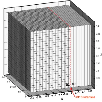
An exemplary mesh for a 3D-1D coupling is depicted in Figure 1.1. The coupling interface between 3D and 1D domain is located atxIF = 0. Consequently, the 3D-mesh and thus the 3D-solver is located atx <0 and the 1D part atx >0. Both domains have the same cross-section in y- and z-direction with no jump in geometry at the coupling interface. The interface connected cells in the 3D part are defined by

with number of cellsNy=Nz=:N for simplicity.

Figure 1.1. Geometry for the 3D-1D coupling, with the 3D mesh on the left and the 1D mesh on the right side of the 3D-1D interface located atxIF = 0.

2.

Interface model for non-cavitating flows

Obviously, a three-dimensional code (based on a three dimensional system) applied on a ”one-dimensional” domain does not behave as a one-dimensional code (based on a one-dimensional system) on the same domain. We want to look for a condition for a three-dimensional code to behave as a one-dimensional code.

2.1.

A necessary and sufficient coupling boundary condition

We use the 3D-1D discretization depicted in Figure 1.1 with the interface atxIF = 0, the cells on the left of interface are referenced by formula (1.5). We assume that the domain{x≥0}is discretized as one dimensional domain by a row of hexahedral cells with volume ∆x×(∆y =: L)×(∆z =: h), the cells are referenced by indexes i fori ≥1 (the celli = 1 touches the interfacexIF = 0 (see Figure 2.1) ). The surfaces of celli are distinguished by the compass-like notationEi(east),Wi (west),Ni (north),Si (south),Ui (upper),Li (lower) as depicted in Figure 2.1.

As the domain{x≥0}is a one dimensional domain, we assume that at any timetn, the cross velocity satisfy

∀i≥1, vn_i =w_in= 0.

We want to deduce a condition which ensures∀i≥1, vn_i+1=w_in+1= 0 at timetn+1=tn+ ∆t forx≥0. Applying a three dimensional Godunov scheme (·)God (see [G1959]) on the third equation of (1.1) on domain

{x >0}(one-dimensional domain), gives

hL∆x[(ρv)n_i+1−(ρv)n_i] + h∆x∆t[(ρv2+p)God_N i −(ρv

2_+p)God Si ]

+hL∆t[(ρuv)God_Ei −(ρuv)God_Wi ] + L∆x∆t[(ρvw)God_Ui −(ρvw)God_Li ] = 0. (2.1)

Using the wall condition (see [BGH2000]) as boundary condition forNi (resp. Si) and defining −−→

NNi (resp.

−−→

NSi) as the unit outward normal vector on the north surface Ni (resp. the south surface Si), the pressure satisfies:

pGod_Ni =pGod(W_in,Wd_Nn i,

−−→

NNi), p

God Si =p

God_(Wn i ,Wd_Sn

i,

−−→

NSi),

where Wd_Nn i =Wd

n Si =Wd

n

i = (ρni,(ρu)ni,−(ρv)ni,(ρw)ni) stands for the mirror state ofWin. As it holds vin = 0 forx >0, we obtainWd_in=W_in, giving

v_NGod i =v

n i =v

God

Si = 0, p

God Ni =p

n i =p

God Si , ρ

God Ni =ρ

n i =ρ

God

Si , (2.2)

with the barotropic equation of state p(ρ, T0). Inserting equation (2.2) to equation (2.1) the second term is

cancelled. With a similar argument for surfaces Ui and Li, we obtain that (ρvw)GodUi = (ρvw)

God

Li = 0 and vGod

Wi = 0. Altogether inserted in equation (2.1), yields

hL∆x(ρv)n_i+1+hL∆t(ρuv)God_E

i = 0. (2.3)

In domainx >∆x,vGod

Ei = 0 holds. Assuming no vacuum (i.e. ρ

n+1

i >0), equation (2.3) providesv n+1

i = 0 for all cells inx >∆x(i.e. i≥2).

For the cell that touches the interface (i.e. i = 1), we obtain a condition for the third component of the numerical fluxes at the interface (xIF = 0) denoted by surfaceEi=1:

vn_i=1+1= 0⇔(ρuv)GodEi=1= 0. (2.4)

The coupling condition can be written as

∀i≥1, v_in+1= 0⇔(ρuv)God_E

i=1 = 0. (2.5)

Further applying the Godunov scheme on the fourth equation of (1.1) gives an equation for the momentum ρw analog to (2.3). Using the same arguments as for equation (2.3), we obtain the condition:

∀i≥1, w_in+1= 0⇔(ρuw)GodEi=1 = 0. (2.6)

Notation 1. (Interface: +,−) Commonly, for the left and the right side of a cell interface the indices ’L’ and ’R’ are used. For general problems, we use this notation. But to denote the coupling interface connected problems, we define ’−’ for the left and ’+’ for the right side of the interface located atxIF = 0(compare Figure

Figure 2.2. The left side of the interfacex < xIF = 0 is denoted by ’−’ and the 3D equations (1.1) are applied. Analog the right side of the interfacex > xIF = 0 is denoted by ’+’ and the 1D equations (1.4) are applied.

The equations (2.5) and (2.6) are the wanted necessary and sufficient coupling boundary conditions to fit to pure one-dimensional simulation in the right domain. The condition depends only on the value of theρv- and theρw- components of the 3D-solver numerical flux at the interfacex= 0+_.

Definition 2. (admissible coupling boundary) A 3D-1D coupling boundary is defined as admissible, if theρv -and theρw- components of the 3D-solver numerical flux at the interface x= 0+ are zero:

(

(ρuv)+= 0,

(ρuw)+_{= 0.} (2.7)

A necessary and sufficient condition for the 3D solver to give a consistent one dimensional numerical flux at the coupling boundary is deduced. To switch at xIF = 0 from the N ×N numerical fluxes F3D(W) := (ρu, ρu2+P, ρuv, ρuw)T (defined in (1.3)) in x-direction at the left side (3D domain) of the interface to one numerical fluxF1D(W) := (ρu, ρu2+P)T (see (1.4)) at the right side (1D domain) of the interface, we want to define a fluxFIF in thex-direction at the interfacexIF = 0 satisfying the coupling condition (2.7).

2.2.

A conservative admissible interface model

Based on the admissible coupling boundary (Definition 2) we develop a conservative admissible interface model. An a priori obvious candidate as a 3D-1D coupling interface model immediately arises considering the projection of the three dimensional Euler equations (1.1) on the plane (O, y, z). We obtain

∂tW+∂xFIF(W) = 0, (2.8)

withW = (ρ, ρu, ρv, ρw) andFIF(W) =F3D(W) = (ρu, ρu2+p, ρuv, ρuw) defined by equations (1.2) and (1.3). The interface model (2.8) does not respect the coupling condition (2.7) and the cross-velocitiesvandwwill not remain zero in the 1D domain as expected (see [HH2007]).

To achieve an admissible interface model, we distinguish the three and one dimensional domain with the function

φ(x, y, z, t) := (

1, x <0,

0, x >0, (2.9)

which does not depend on timetand vanishes for the 1D domain assumed forx >0 and we insertφto equation (2.8). We receive the admissible interface model

∂tY +∂xFIF(Y) = 0, (2.10)

with the vector of conservative variablesY := (φ, WT₎T _{= (φ, ρ, ρu, ρv, ρw)}T _{and fluxesF}

IF(Y) := (0, ρu, ρu2+ p, φρuv, φρuw)T _{(compare [HH2007]: Y := (φ, ρ, u, v) or (φ, ρ, u, ρu)). The jump function φ(x > 0, y, z, t) :=} φ+_{= 0 vanishes at the ’+’-side of the interface. Thus the fluxF}+

2.3.

Numerical scheme

We apply the 3D and 1D solver on the 3D resp. 1D domain and use the admissible interface model (2.10) to model the numerical fluxesF_IF± over the interface. We describe the Riemann problem at the interface in detail. On the 3D or ’−’-side of the interface we have the left states of the interface Riemann problem defined by

Y_i,j,k3D := (φ= 1, ρ, ρu, ρv, ρw)i,j,k= (1, ρ, ρu, ρv, ρw)i,j,k (2.11)

for (i, j, k) defined in (1.5) and the 1D or ’+’-side we have the right state

Y_i1₌₁D:= (φ= 0, ρ, ρu, ρv= 0, ρw= 0)i=1= (0, ρ, ρu,0,0)i=1. (2.12)

For the ’−’-side, we need to compute the numerical fluxes

F_IF− :=F(Y_i3₌₀D_,j,k, Y_i1₌₁D,0−)

betweenY3D

i=0,j,k and Y

1D

i=1 forj, kdefined in (1.5). As the size of the cross-section (in y andz) at the interface

xIF = 0 is the same for the ’−’-side and the ’+’-side, the finite volume scheme together with the Green formula give us thatF_IF+ is the sum of all local fluxesF(Y3D

i=0,j,k, Y

1D

i=1,0+) inx- direction by assumingN equally spaced

gridcells on the ’−’-side and one cell on the ’+’-side of the interface:

F_IF+ := X

j=0,..,Ny;k=0,..Nz

F(Y_i3₌₀D_,j,k, Y_i1₌₁D,0+). (2.13)

To receive a consistent numerical 3D-1D coupling method, we use the same finite volume scheme for the cells connected to the interface xIF = 0 as in the interior cells of the 3D and 1D domains. But to compute the numerical fluxes F_IF± at the interface xIF = 0, we solve the Riemann problem between the left state Y− =Y_i3₌₀D_,j,k and right stateY+ =Y_i1₌₁D using (2.10) instead of the two original models (1.1) for the 3D and (1.4) for the 1D part. For the calculation of the numerical fluxes F_IF± at the interfacexIF = 0 we consider two Riemann-based schemes: Catum scheme and a Roe-type scheme to solve the Riemann problem between (2.11) and (2.12).

2.3.1. Catum scheme

An obvious candidate for the numerical flux calculation is the Riemann-like flux formulation Catum, as used in the interior cells of the 1D and 3D part. The advantage of Catum in comparison with other Riemann-based schemes for the simulation of evolution of cavitation is the uniformly consistency with respect to Mach number. The common used numerical approximation of the cell interface pressure

p∗=pL+pR 2 +

ρL,RcL,RuL,R N

is based on compatibility relations and is not uniformly consistent with respect to Mach number. To achieve a uniform consistency in Mach number the numerical fluxes are defined for the admissible conservative interface model (2.10) by

F_IF±,Catum=ρLu∗·(0,1, u∗, φ·vL, φ·wL)T+p∗·(0,0,1,0,0)T, with the transport velocityu∗ and the pressurep∗

u∗:= ρLcLuL+ρRcRuR+pL−pR ρLcL+ρRcR

, p∗:= pL+pR 2 .

consistent with respect to multidimensional low Mach number flows. For details see [SSST2008]. The Catum scheme has a high numerical dissipation (influence on coupling results see section 2.4), thus as second scheme, a Roe-type scheme, with low dissipation is considered.

2.3.2. Roe-type scheme

The interface model (2.10) can be written in condensed form as

∂tY +J(Y)∂xY = 0, (2.14)

with the matrix J(Y) given by

J(Y) = 

    

0 0 0 0 0

0 0 1 0 0

0 −u2_+c2 _{2u 0 0}

ρuv −φuv φv φu 0 ρuw −φuw φw 0 φu



    

and the speed of soundc which verifies

c2=p0(ρ)>0. (2.15)

For system (2.14) the eigenvalues λj, the right-eigenvectors rj and the normalized left-eigenvectors lj of the matrixJ(Y) (extending the results of [HH2007] byφwand use conservative variables) can be analytically calculated by

λ1= 0, r1= (φ,0,0,−ρv,−ρw)T

λ2=u−c, r2= (0,−u+c+φu,(u−c)(−u+c+φu), φvc, φwc)T

λ3=λ4=φu,

(

r3= (0,0,0,1,0)T

r4= (0,0,0,0,1)T

λ5=u+c, r5= (0, u+c−φu,−(u+c)(−u−c+φu), φvc, φwc)T

λ1= 0, l1=

₁

φ,0,0,0,0

λ2=u−c, l2=

0, −u−c

−2c2_{−2cφu+ 2uc},

1

−2c2_{−2cφu+ 2uc},0,0

λ3=λ4=φu,

( l3=

ρv

φ,−

(φu2_−u2_−c2_)φv

φ2u2+u2₋c2₋2φu2,

φuv(φ−1)

φ2u2+u2₋c2₋2φu2,1,0

l4= 0,0,0,−w_v,1

λ5=u+c, l5=

0, c−u 2c2_{−2cφu+ 2uc},

1

2c2_{−2cφu+ 2uc},0,0

.

The first, third and fourth fields are linearly degenerate while the second and the fifth are genuinely non-linear. In comparison with the original Euler equations an additionally stationary waveλ1= 0 at the interfacexIF = 0 exists for the conservative interface model (2.10).

Definition 3. For the linearisation of the Riemann problem (2.14) we define the vector of averages Yb := (φ,b _bρ,ρu,_{c c}ρv,ρw)_c T. We recall the original Roe averages ρ,_bu,_{b b}v,w_b:

b

ρ=√ρRρL, u_b= √

ρRuR+ √

ρLuL √

ρR+ √

ρL

, _bv=

√

ρRvR+ √

ρLvL √

ρR+ √

ρL

, w_b=

√

ρRwR+ √

ρLwL √

ρR+ √

ρL ,

and define the averages_bc andφbby

b c =

(cL+cR

2 =cL=cR , if4ρ= 0,

q

4p

4ρ , if4ρ6= 0 , b φ =            1

2 , if uL= 0,

1− √

ρR(

√ ρRuR+

√ ρLuL)

uL(

√ ρR+

√

ρL)2 , if uL6= 0and0<

√ ρR(

√ ρRuR+

√ ρLuL)

uL(

√ ρR+

√

ρL)2 <1,

1 , if uL6= 0and

√

ρR(√ρRuR+√ρLuL)

uL(

√ ρR+

√

ρL)2 <0,

0 , if uL6= 0and

√ ρR(

√ ρRuR+

√ ρLuL)

uL(

√ ρR+

√

ρL)2 >1.

We define as initial condition

(

vR=wR= 0,

φL= 1, φR= 0.

(2.16)

with φdefined in (2.9)and ’L’, ’R’ defined in Notation 1. Furthermore we define4(·) := (·)R−(·)L.

The linearized Riemann problem is defined by

∂tY +J( ˆY)∂xY = 0, (2.17)

withY := (φ, ρ, ρu, ρv, ρw)T_{, the Roe-averages} b

Y :=φ,b _bρ,ρu,_{c c}ρv,ρw_c T

and the initial condition

Y(x,0) = (

YL , x <0,

YR , x >0.

(2.18)

We denote the solution of (2.17)-(2.18) byY YL, YR, x_t ±

. If we apply a Roe-type scheme for calculating the

Riemann fluxes through the coupling interface, we consider the solution at x_t = 0:

Y YL, YR,0±. (2.19)

Proposition 4. If the linearized Riemann problem (2.17)-(2.18)fulfills

4FIF(Y) =4       0 ρu ρu2+p

φρuv φρuw      

=4JYb

Y=JYb

4Y (2.20)

the difference between the flux on the left F_IF− and on the rightF_IF+ side of the interface is exactly preserved.

Proof. For the second component of4FIF(Y) an easy computation gives4(ρu) =ρb4u+ub4ρ. For the third component, we have to prove

Using the result for the second component4(ρu), we obtain

−u_b24ρ+ 2u_b4(ρu) = u(_b 4(ρu) +ρ_b4u) = u((ρu)_b R−(ρu)L+

√

ρRρL(uR−uL))

= u(_b √ρRuR( √

ρR+ √

ρL)− √

ρLuL( √

ρR+ √

ρL))

= (√ρRuR+ √

ρLuL)( √

ρRuR− √

ρLuL)

= ρRu2R−ρLu2L

= 4(ρu2).

⇒ 4(ρu2+p) = 4(ρu2) +_bc24ρ.

Finally, equation (2.21) is satisfied

• for4ρ= 0, if 4p= 0. This condition is fulfilled as we use the same equation of state on both sides of the interface and we defined_bc in Definition 3 as_bc:= 0.5∗(cL+cR) =cL=cR,

• for4ρ6= 0, if_bc2₌4p

4ρ holds as given in Definition 3 and using equation (2.15).

For the fourth component of4FIF(Y), the relation

4(φρuv) =ρ_bbu_bv4φ−φbu_bv_b4ρ+φb_bv4(ρu) +φbu_b4(ρv), (2.22)

has to be verified. We have

(2.22) ⇔ 4(φρuv)−ρ_bbuv_b4φ= (−_bu_bv4ρ+_bv4(ρu) +_bu4(ρv))bφ

⇔ 4(φρuv)−ρ_bbuv_b4φ= (u_bbv4ρ+ρ_bv_b4u+ρ_bu_b4v)bφ.

If we use the initial condition (2.16), a long (but not difficult) computation gives

(

4(φρuv)−ρ_bu_bbv4φ=−ρLuLvL−

ρLvL√ρR(√ρRuR+√ρLuL)

(√ρR+

√

ρL)2 4φ,

b

u_bv4ρ+ρ_bv_b4u+ρ_bu_b4v=−ρLuLvL,

and then we obtain

(2.22) ⇔ −ρLuLvL− ρLvL

√

ρR( √

ρRuR+ √

ρLuL) (√ρR+

√

ρL)2

4φ=−ρLuLvLφ.b

Furthermore,φbis solution of (2.22), ifφbsatisfies

−ρLuL− ρL

√

ρR( √

ρRuR+ √

ρLuL) (√ρR+

√

ρL)2

4φ=−ρLuLφ,b (2.23)

and the fifth equation of 4FIF(Y). Replacingv byw the same calculation gives us thatφbhas again to fulfill equation (2.23). To fulfill equation (2.23),

• ifuL6= 0, we chooseφb= 1 +

√ ρR(

√ ρRuR+

√ ρLuL)

uL(

√ ρR+

√

ρL)2 4φand the relation (2.20) is satisfied because it yields

4φ=−1 at the interface. As definedφ∈[0; 1], it seems natural to chooseφb∈[0; 1] and we define:

b φ =        1− √

ρR(

√ ρRuR+

√ ρLuL)

uL(√ρR+√ρL)2 , if0<

√ ρR(

√ ρRuR+

√ ρLuL)

uL(√ρR+√ρL)2 <1,

1 , if

√ ρR(

√ ρRuR+

√ ρLuL)

uL(

√ ρR+

√

ρL)2 <0,

0 , if

√ ρR(

√ ρRuR+

√ ρLuL)

uL(√ρR+√ρL)2 >1.

Remark 5. This proof is only valid for the initial condition (2.16) because in this caseφbdoes not depend on v

andw. We recall that if uL= 0 and if uR6= 0, the relation (2.22) will not be verified and the condition (2.20)

is not preserved, but only a small error occurs.

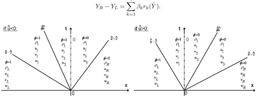
Solution of the linearized problem. The construction of the solution of the linearized Riemann problem (2.17)-(2.18) is classical, but we briefly recall it for an easy implementation of the Roe-type scheme.

Given the eigenvalues λk( ˆY) with k = 1, . . . ,5 (depicted in Figure 2.3) and the associated right eigenvectors rk( ˆY), we computeβk such that:

YR−YL=

5

X

k=1

βkrk( ˆY).

Figure 2.3. Characteristics and states of the linearized Riemann problem of the thin interface model considered at the interface withk= 4 =:Landk= 5 =:R.

The solution of the linearized Riemann problem (2.17)-(2.18) is given by:

Y(x, t) =YL+ X

x t<λl(Yb)

βlrl(Yb).

In order to calculate the solutionY(x, t), we need to computeβ1,β2andβ5:

β1=

φR−φL

b

φ , β2= 1 2

ˆ u+_bc

b

c(_bc−_bu+φb_bu)

(ρR−ρL)− 1 2

1

b

c(_bc−_bu+φb_bu)

((ρu)R−(ρu)L),

β5=

1 2

ˆ u−_bc

b

c(−_bc−u_b+φbu)_b

(ρR−ρL)− 1 2

1

b

c(−_bc−u_b+φb_bu)

((ρu)R−(ρu)L).

• ifλ2( ˆY)>0, thenY(YL, YR,0−) =YL andY(YL, YR,0+) =YL+β1r1(Yb),

• if λ2( ˆY) < 0 and λ3( ˆY) = λ4( ˆY) > 0, then Y(YL, YR,0−) = YL +β2r2( ˆY) and Y(YL, YR,0+) = YL+β1r1( ˆY) +β2r2( ˆY),

• ifλ3( ˆY) =λ4( ˆY)<0 andλ5( ˆY)>0, thenY(YL, YR,0−) =YR−β5r5( ˆY)−β1r1( ˆY) andY(YL, YR,0+) = YR−β5r5( ˆY),

• ifλ5( ˆY)<0, thenY(YL, YR,0−) =YR−β1r1( ˆY) andY(YL, YR,0+) =YR.

Numerical flux and entropy correction. To compute the numerical fluxFIF(Y(Yin, Yin+1,0±)), we know the

interface statesY(Yn

L, YRn,0±) defined in equation (2.19) as solution of the linearized Riemann problem (2.17), we can use the barotropic equation of statep(ρ, T0) to determine the pressurep(0±) at the interface. The Roe

scheme without entropy correction can predict wrong waves and thus authorizes non-physical shocks crossing the interface. It occurs when between two cells Ωi and Ωi+1 an eigenvalue is associated to a non linear k-field:

λk(YLn)≤0 ≤λk(YRn). If and only if a smooth rarefaction wave develops, an entropy correction to guarantee the second principle of thermodynamics is needed. Many numerical entropy corrections exist (e.g. [HH1983]). The approach presented here consists in increasing locally the numerical viscosity of the scheme, as presented in [HHMS2010]. The advantage of this correction is that it is lipschitzian if the numerical flux is lipschitzian.

Definition 6. (Entropy correction) If λk(YLn)≤0≤λk(YRn)and k-field is non linear, then the numerical flux FIF is replaced by:

FIF(Y(YLn, Y n

R,0±)) =FIF(Y(YLn, Y n

R,0±))−min k (|λk(Y

n

L)|,|λk(YRn)|) Yn

R −Y n L 2 .

Consequently, with the interface marking functionφ(x, y, z, t) and the admissible coupling boundary condition (2.7), we have a conservative admissible interface model (2.10), which belongs to the thin interface models. Thus the 3D Euler method can be coupled with the 1D Euler method for non-cavitating flows using the interface model (2.10). The details needed for implementing the Catum and Roe-type scheme are given in section 2.4.

Notation 7. The interface model (2.10) belongs to the thin interface models (compare [HH2007]) and is called

TI. Applying the Catum (see section 2.3.1) or the Roe-type scheme (see section 2.3.2) we define the resulting method as TICatumor TIRoe.

2.4.

Numerical results

The coupling algorithms TICatum and TIRoe for non-cavitating flow passing the interface at xIF = 0 are compared to each other and the pure 3D solution calculated by 3D Catum. The domain depicted in Figure 1.1 is decomposed by ∆x= ∆y= ∆ztoN×N×N equidistant hexahedral gridcells for the pure 3D simulation. For the couplings TICatum or TIRoe the geometry is divided into two parts by locating the interface atxIF = 0, the 3D mesh forx <0 withNx,3D×N×N and the 1D mesh forx >0 withNx,1D×1×1 andN :=Nx,3D+Nx,1D number of gridcells. We recall, that for the same cross-section (y- andz-direction) at the interface, there is no jump in geometry at the interface.

As initial condition we assumepinit >> psat andu=v=w= 0, with psat saturation pressure defined by the equation of state and pinit the initial pressure. To introduce a pressure wave passing the 3D-1D interface at xIF = 0 one or two small regions with a pressurepmax> pinitare initialised. The corresponding densityρ(p, T0)

is obtained using the barotropic equation of state for a diesel-like test-fluid. All boundaries are assumed as walls. The internal cut of the geometry atxIF = 0 for the coupled simulation is modelled by TICatum or TIRoe and the 3D or 1D part is simulated by the 3D or 1D Catum. With this setup, the necessary and sufficient interface coupling condition (2.7): (ρuv)+ = (ρuw)+ = 0 is fulfilled. Both codes use a cfl 1.0 and to assure synchro-nous timestepping, the minimum of the valid timestep of the 1D and 3D code is used as timestep for both codes.

Remark 8. In the following, we only consider the solutions for the x- and y-direction. The results for the z -direction are the same as for they-direction and are neglected. The results of Figure 2.5 - 2.8 show the solution at the simulation timet1>0 ort2> t1, corresponding to the time when the wave reaches the interface.

2.4.1. Testcase 1: Non-cavitating flow with zero averaged cross-velocities

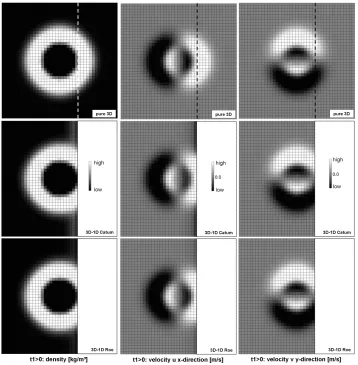
By introducing one pressure peakpmax as initial condition, we receive a pressure wave, which travels over the interface depending on timet. As depicted in Figure 2.5 at timet1>0, the primitive variables are

approx-imated very well by the TIRoe scheme in comparison to the pure 3D solution. The assumption of the constant 1D-values ρ1D, u1D, p1D(ρ) and the cross-velocity v1D = 0 as constant right state of the local 3D Riemann problems at the interface xIF = 0 for the computation of the fluxes FIF± over the interface, implicates small artificial jumps within each local Riemann problem and thus leads to an error in the 3D-1D solution. Especially with the interface model TICatum this error can be detected in the interface connected cells of the 3D part for the velocityu. We achieve a direct comparison of the 1D part solution and the pure 3D solution by averaging the 3D solution with respect to the x-axis. As depicted in Figure 2.6, all results fit very well, with only a small influence in the vicinity of the interface located atxIF = 0.

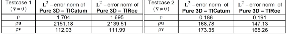
In Figure 2.4 theL2_{−errors for the densityρ, the momentum inx-directionρuand iny-directionρvcalculated}

with the solver TICatum and TIRoe in comparison with the pure 3D solutions, based on the averaged values depicted in Figure 2.6, are shown. The solutions calculated with the two different flux formulations Catum and Roe are almost the same. Concluding, this testcase illustrates that the interface models TIRoe and TICatum introduce only small errors to the flow in the vicinity of the interface. As shown in the averaged solutions in Figure 2.6, the averaged momentum iny-directionρv= 0 is zero for the 1D part and thus the solution of φρv at the interface coincides with the model assumption (φρuv)+ _{= 0. A setup with ρv 6= 0 at the interface is}

considered in the second testcase.

Figure 2.4. L2-error for the solver TICatum and TIRoe in comparison with the pure 3D solution at time t1 for testcase 1 (see left side and section 2.4.1) and timet2 > t1 for testcase

2 (see right side and section 2.4.2).

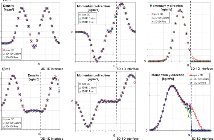
2.4.2. Testcase 2: Non-cavitating flow with non-zero averaged cross-velocities

To achieve a non-zero averaged cross-velocity, two pressure peaks pmax are initialised at different xand y locations in the 3D part within the geometry given in Figure 1.1, to obtain an asymmetric cross-velocity field. With this flow field, the strength of influence of the model assumption (ρuv)+_{= 0 of the thin interface model TI}

can be observed. As shown in Figure 2.7 on the left row, at timet1>0 the densitiesρhave the same predicates

as in the first testcase (see section 2.4.1). To approximate the velocityvin the 1D part, we assumev1D= 0. In the right plot of Figure 2.8 we clearly see, that this assumption is fulfilled. The condition (ρuv)+= 0 leads to a zeroρv-flux over the interface, thus the momentum in y-direction jumps between the last cell layer of the 3D-and the first cell in the 1D-part. But we also detect an error in the averagedy-momentum at timet2for TIRoe

Figure 2.5. Non-cavitating testcase with zero average velocities.

Figure 2.7. Non-cavitating testcase with non-zero cross-velocities.

Figure 2.8. Non-cavitating testcase with non-zero cross-velocities at timet1>0 andt2> t1.

3.

Interface model for cavitating flows

Based on the admissible conservative coupling interface model (2.10) for non-cavitating flow passing the interface, an extension to cavitating flow is developed. The limit of interface model (2.10) with respect to cavitating flow passing the interface, is the calculation of the flux for the 1D solver at the interface. An addition of the local three dimensional fluxes is performed (see equation (2.13)), which is not valid for local two-phase regions. The equation of state is non-linear in the two-phase region in comparison with the linear liquid region, which leads to inconsistent densities in the 1D flux for local cavitation regions in the 3D domain at the interface xIF = 0. A model considering the local vapor fraction at the interface is needed and developed in this section by splitting the homogeneous densityρ=αρliq+ (1−α)ρvap (whereαis the volume fraction of liquid) to its liquidρliq and vaporρvap ratio. Splitting the homogeneous density, the original equation of state is valid over the interface for cavitating flows and cavitation bubbles can pass the interface. We recall that the interface model is only applied for the interface connecting cells. The other fluxes inside the domain are computed by the 3D respectively 1D Catum scheme.

3.1.

Governing equations

The same barotropic equation of state for a diesel-like test-fluid as mentioned above is used and it is given by a table, which includes the pressurepas function of the homogeneous densityρ, the liquid densityρ1:=ρliq and the vapor density ρ2:=ρvap and the volume fraction of the liquid phaseαwith the homogeneous density ρ=αρ1+ (1−α)ρ2. This table gives unique pressure lawsp1=p1(ρ1, T0) andp2=p2(ρ2, T0). We are able to

consider the ideas described in [CCJK2006] as extension of the interface model (2.10) fulfilling equation (2.7), where the mass conservation is split into two equations coupled by a source term. We define the following interface model:

(

∂t( ˜W) +∂xF˜IF( ˜W) +∂yG˜IF( ˜W) +∂zH˜IF( ˜W) = ˜SIF( ˜W) ∂tα+u∂xα+v∂yα+w∂zα=k(p1(ρ1)−p2(ρ2)),

(3.1)

where

˜

W = (φ, m1, m2, ρu, ρv, ρw)T,

˜

FIF( ˜W) = (0, m1u, m2u, ρu2+p, φρuv, φρuw)T,

˜

GIF( ˜W) = (0, m1v, m2v, ρuv, ρv2+p, ρvw)T,

˜

HIF( ˜W) = (0, m1w, m2w, ρuw, ρvw, ρw2+p)T,

˜

SIF( ˜W) = (0, λ(g2(ρ2)−g1(ρ1)),−λ(g2(ρ2)−g1(ρ1)),0,0,0)T,

withα= V1

Vtot the volume fraction of the liquid phase,mi=

Mi

Vtot (withMi the mass of phasei= 1,2), ρi =

Mi

Vi the density of each phase, φis define by (2.9), gi is the free enthalpy of each phase, that satisfies _dρdg_ii = _ρ1_idp_dρi_i and the pressure lawp=αp1(ρ1) + (1−α)p2(ρ2).

Remark 9. If we add the second and the third equations of system (3.1), we obtain∂tρ+∂x(ρu) = 0, which is

the equation of mass conservation. The source terms cancel because of the opposite signs. The last equation of (3.1) can also be written as

∂t(αρ) +∂x(αρu) +∂y(αρv) +∂z(αρw) =kρ(p1(ρ1)−p2(ρ2)). (3.2)

The splitting of the mass conservation and using a source term, considers the vapor density ρ2 separately

from the liquid densityρ1. Using this splitting, we can perform a valid addition of fluxes (2.13) at the interface

3.1.1. Properties of model (3.1)

For smooths solutions ˜Y, we can write system (3.1) in condensed form

∂tY˜ +Jx( ˜Y)∂xY˜ +Jy( ˜Y)∂yY˜ +Jz( ˜Y)∂zY˜ = ˜SIF( ˜Y), (3.3)

where ˜Y = (φ, m1, m2, ρu, ρv, ρw, α)T = ( ˜WT, α)T, ˜Sφ( ˜Y) = ( ˜S3D( ˜W)T, k(p1(ρ1)−p2(ρ2)))T and matrixJx( ˜Y), Jy( ˜Y) andJz( ˜Y) are given by

Jx( ˜Y) =          

0 0 0 0 0 0 0

0 uy2 −uy1 y1 0 0 0

0 −uy2 uy1 y2 0 0 0

0 c2

1−u2 c22−u2 2u 0 0 N

ρuv −φuv −φuv φv φu 0 0 ρuw −φuw −φuw φw 0 φu 0

0 0 0 0 0 0 u

         

, Jy( ˜Y) =          

0 0 0 0 0 0 0 0 vy2 −vy1 0 y1 0 0

0 −vy2 vy1 0 y2 0 0

0 −uv −uv v u 0 0 0 c2

1−v2 c22−v2 0 2v 0 N

0 −vw −vw 0 w v 0 0 0 0 0 0 0 v

          ,

Jz( ˜Y) =          

0 0 0 0 0 0 0

0 wy2 −wy1 0 0 y1 0

0 −wy2 wy1 0 0 y2 0

0 −uw −uw w 0 u 0 0 −vw −vw 0 w v 0 0 c2

1−w2 c22−w2 0 0 2w N

0 0 0 0 0 0 w

          ,

whereyi= M_Mi =m_ρi,c2i = dpi

dρi is the squared sound velocity of each phases withi= 1,2 andN =

∂p

∂α. Denoting bycthe speed of sound of the mixture, it yields c2_=y

1c21+y2c22.

To study system (3.3), we have to examine the three matrices Jx( ˜W),Jy( ˜W) andJz( ˜W). The eigenvalues λx,j=1,..,7, right-eigenvectorsrx,j=1,..,7and left-eigenvectorslx,j=1,..,7of the matrix Jx( ˜Y) are

λx,1= 0, rx,1= (φ,0,0,0,−ρv,−ρw,0)T,

lx,1= (

1

φ,0,0,0,0,0,0),

λx,2=u−c, rx,2= (0, y1, y2, u−c,

φvc

−u+c+φu,

φwc

−u+c+φu,0) T_,

lx,2= (0,

uc+c2 1

2c2 ,

uc+c2 2

2c2 ,−

1 2c,0,0,

N 2c2),

λx,j=3,4=u,

(

rx,3= (0,1,0, u,0,0,−

c2₁ N)

T

rx,4= (0,0,1, u,0,0,−

c2 2

N)

T ,

(

lx,3= (0,

y2c22

c2 ,−

y1c22

c2 ,0,0,0,−

N y1

c2 )

lx,4= (0,−

y2c21

c2 ,

y1c21

c2 ,0,0,0,−

N y2

c2 )

,

λx,j=5,6=φu,

(

rx,5= (0,0,0,0,1,0,0)T

rx,6= (0,0,0,0,0,1,0)T

,

(

lx,5= (ρv_φ, (c2

1+u2(1−φ))φv

u2_−c2_+φu2_(φ−2),

(c2

2+u2(1−φ))φv

u2_−c2_+φu2_(φ−2),

uvφ(1−φ)

u2_−c2_+φu2_(φ−2),1,0,

N φv u2_−c2_+φu2_(φ−2))

lx,6= (0,0,0,0,−w_v,1,0)

,

λx,7=u+c, rx,7= (0, y1, y2, u+c,

φvc u+c−φu,

φwc u+c−φu,0)

T_,

lx,7= (0,

c2 1−uc

2c2 ,

c2 2−uc

2c2 ,

1 2c,0,0,

The eigenvaluesλy,j=1,..,7, right-eigenvectorsry,j=1,..,7 and left-eigenvectorsly,j=1,..,7of the matrix Jy( ˜Y) are

λy,1= 0, ry,1= (1,0,0,0,0,0,0)T, ly,1= (1,0,0,0,0,0,0),

λy,2=u−c, ry,2= (0, y1, y2, u, v−c, w,0)T, ly,2= (0,

vc+c2 1

2c2 ,

vc+c2 2

2c2 ,0,−

1 2c,0,

N 2c2)

λy,j=3,4,5,6=v,

          

ry,3= (0,0,0,1,0,0,0)T

ry,4= (0,0,0,0,0,1,0)T

ry,5= (0,1,0,0, v,0,−

c2 1

N) T

ry,6= (0,0,1,0, v,0,−

c2 2 N) T ,           

ly,3= (0,−

uc2 1

c2 ,−

uc2 2

c2 ,1,0,0,−

N u c2 )

ly,4= (0,0,0,−w_u,0,1,0)

ly,5= (0,

y2c22

c2 ,−

y1c22

c2 ,0,0,0,−

N y1

c2 )

ly,6= (0,0,0,0,−w_v,1,0)

λy,7=u+c, ry,7= (0, y1, y2, u, v+c, w,0)T, ly,7= (0,

c21−vc

2c2 ,

c22−vc

2c2 ,0,

1 2c,0,

N 2c2),

The second and seventh field are genuinely non-linear while others are linearly degenerated.

For eigenvaluesλz,j=1,..,7, right-eigenvectorsrz,j=1,..,7 and left-eigenvectorslz,j=1,..,7 of the matrixJz( ˜Y) we obtain a similar formula as for matrixJy( ˜Y).

3.2.

Numerical scheme

To solve system (3.3) with source term ˜SIF( ˜Y), we firstly solve the conservative part of (3.3) and secondly, we take the source term into account.

Definition 10. (M-equilibrium condition) The M-equilibrium condition is fulfilled, if the pressure of the liquid phasep1 in a gridcelli is the same as the pressure of the vapor phasep2:

p1(ρ1) =p2(ρ2). (3.4)

The M-equilibrium condition is formally equivalent to suppose k → ∞ in system (3.1) (see [CCJK2006] for details).

The M-equilibrium algorithm is subdivided into the following steps.

(1) Conservative part. Solve the conservative part of equation (3.3) with a finite volume scheme between time steptn andtn+1.

• Update ˜W with a Roe-type scheme and obtain ˜Wn+1/2.

• Updateαwith an upwind scheme (see below) and obtain αn+1/2. As result receive ˜Yn+1/2= (( ˜Wn+1/2)T, αn+1/2)T.

(2) Source term. Consider the source term ˜SIF( ˜Y) with the M-equilibrium condition (3.4). An ordinary differential equation (3.9) has to be solved in [0; ∆t] with the initial condition ˜Yn+1/2= ˜Y(x, y, z,0). (3) Update α. Updateαsuch that it satisfies the M-equilibrium (3.4).

3.2.1. First step: Conservative part

In this step, we want to solve the conservative part of system (3.3)

(

∂t( ˜W) +∂xF˜IF( ˜W) +∂yG˜IF( ˜W) +∂zH˜IF( ˜W) = 0

∂tα+u∂xα+v∂yα+w∂zα= 0,

(3.5)

with an explicit first order finite volume scheme. The fluxes ˜GIF and ˜HIF are computed with a classical Roe solver (see e.g. [CCJK2006]). The interface flux ˜FIF contains the function φ and thus has to be explained.

Proposition 11. The classical Roe averagesρ_b,_bu,_bv andw_b are defined as

b

ρ=√ρRρL, u_b= √

ρRuR+ √

ρLuL √

ρR+ √

ρL

, _bv=

√

ρRvR+ √

ρLvL √

ρR+ √

ρL

, w_b=

√

ρRwR+ √

ρLwL √

ρR+ √

ρL .

Assume y_bi as

b yi=

√

ρRyi,R+ √

ρLyi,L √

ρR+ √

ρL

, i= 1,2

and assume that there existscb2_i andNb such that the following discrete jump condition is verified

4p= X i=1,2

b c2

i4(mi) +Nb4α.

If the initial condition is

(

vR=wR= 0,

φL= 1, φR= 0,

(3.6)

andφbis defined as

b φ=

(₁

2 , if uL= 0

1− √

ρR(

√ ρRuR+

√ ρLuL)

uL(

√ ρR+

√

ρL)2 , if uL6= 0,

the relation

4F˜IF( ˜W) 4α

=Jx(Yb˜)4Y˜

is satisfied. Thus the difference of the flux on the left F_IF− and on the rightF_IF+ side of the interface of system

(3.3)is exactly preserved.

Proof. The proof is similar to the proof of proposition 4 and thus is not given.

Remark 12. As for Proposition 4, the proof is only valid for the initial conditions (3.6) because in this case φb

does not depend onv andw, we recall that ifuL= 0and if uR6= 0, the jump relation forφbwill not be verified

(see Proposition 4).

To compute the interface flux ˜FIF, we have to find the solution ˜Y( ˜YL,Y˜R,0±) of the linearized Riemann problem:     

∂tY˜ +Jx(Yb˜)∂x( ˜Y) = 0,

˜

Y(x,0) = (

˜

YL, if x <0, ˜

YR, if x >0,

(3.7)

which is

˜

Y(x, t) = ˜YL+ X

x

t<λx,l(Yb˜)

To calculate the solution ˜Y, we need to identifyβx,k with k= 1,2,3,4,7, as explained for the eigenvectors ofJx in section 3.1.1:

βx,1=

1

b φ4φ

βx,2=

b c2

1+ubbc 2cb2

4(m1) +

b c2

2+ubbc 2cb2

4(m2)−

1

2_bc4(ρu) + b N

2cb2

4α,

βx,3= b

y2cb2₂

b

c2 4(m1)−

b y1cb2₂

b

c2 4(m2)−

b y1Nb

b c2 4α,

βx,4=−b

y2cb2₁

b

c2 4(m1) +

b y1cb2₁

b

c2 4(m2)−

b y2Nb

b c2 4α,

βx,7=

b c2

1−ubbc 2cb2

4(m1) +

b c2

2−ubbc 2cb2

4(m2) +

1

2_bc4(ρu) + b N

2cb2

4α.

The interface states are then defined by

• ifλx,2(Yˆ˜)>0, then ˜Y( ˜YL,Y˜R,0−) = ˜YL and ˜Y( ˜YL,Y˜R,0+) = ˜YL+βx,1rx,1(Yb˜),

• ifλx,2(Y˜ˆ)<0 andλx,3(Y˜ˆ) =λx,4(Yˆ˜)>0, then ˜Y( ˜YL,Y˜R,0−) = ˜YL+βx,2rx,2(Yˆ˜) and ˜Y( ˜YL,Y˜R,0+) = ˜

YL+βx,1rx,1(Y˜ˆ) +βx,2rx,2(Yˆ˜),

• if λx,3(Y˜ˆ) =λx,4(Yˆ˜)<0 and λx,7(Yˆ˜)>0, then ˜Y( ˜YL,Y˜R,0−) = ˜YR−βx,7rx,7(Yˆ˜)−βx,1rx,1(Yˆ˜) and

˜

Y( ˜YL,Y˜R,0+) = ˜YR−βx,7rx,7(Yˆ˜),

• ifλx,5(Yˆ˜)<0, then ˜Y( ˜YL,Y˜R,0−) = ˜YR−βx,1rx,1(Yˆ˜) and ˜Y( ˜YL,Y˜R,0+) = ˜YR.

Now the three fluxes ˜F3D, ˜H3D and ˜G3D can be calculated and we can update ˜W. To finish the first step, we have to updateαusing the second equation of system (3.5) and the following upwind scheme:

αn_i+1/2=αn_i − ∆t

2∆x((bu n i− |bu

n i |)(α

n i+1−α

n i) + (bu

n i+|bu

n i |)(α

n i −α

n

i−1)). (3.8)

3.2.2. Second step: Source term We integrate the ODE system:

(

∂t( ˜W) = ˜SIF( ˜W)

∂tα=k(p1(ρ1)−p2(ρ2)),

(3.9)

over [0;4t] with the initial condition

˜

Y(x, y, z,0) = ˜Yn+1/2(x, y, z,0).

We assume the M-equilibrium (3.4), which means that the last component of the source term kρ(p1(ρ1)−

p2(ρ2)) = 0 is zero or similarly we suppose thatαis chosen such that

p1

m₁ α

=p2

_m

2

1−α

, (3.10)

using the pressure lawsp1(ρ1, T0) andp2(ρ2, T0). With assumption (3.10), system (3.9) is transferred to

(

∂t( ˜W) = ˜SIF( ˜W)

∂tα= 0.

We deduce an approximate ODE system that allows explicit integration instead of a direct numerical integration of system (3.11) to assure stability and maximum principle purpose. Therefore, we scale parameterλby setting λ=m1m2λ, whereλis supposed to be a large constant and we fix the (g2−g1) term as (g2−g1)n+1/2evaluated

at ˜Y_in+1/2. We obtain the simplified ODE system

∂t(m1) =m1m2λ(g2−g1)

n+1/2

i =m1(ρ

n+1/2

i −m1)λ(g2−g1)

n+1/2

i , ∂t(ρ) = 0, ∂t(ρu) = 0,

which can be solved explicitly

m1(t) =

ρn_i+1/2

ρn_i+1/2

(m1)ni+1/2

−1

exp−λtρn_i+1/2(g2−g1)

n+1/2

i

+ 1

, ρ(t) =ρn_i+1/2, u(t) =un_i+1/2.

Let us notice that the above relation ensures m1(t) ∈ [0;ρ(t)] for all t > 0. We now complete the source

integration step by setting

ρ_in+1=ρ_in+1/2, un_i+1=u_in+1/2, (m1)ni+1=m1(4t), (m2)ni+1=ρ n+1

i −(m1)ni+1.

3.2.3. Third step: Updateα

We update αby remappingαinto the M-equilibrium states (3.4). In fact,αn+1 is the solution of equation (3.10), then we finally obtain

p1

_mn+1 1

α

=p2

_mn+1 2

1−α

.

Remark 13. The ”cavitating” interface model (3.3)is not conservative as the admissible conservative interface model (2.10) for non-cavitating flows. But the interface model (3.3)is valid for cavitating and non-cavitating flow passing the interface. The error received at the interface depends on the amount of cavitation bubbles passing the interface. But this model ensures the same pressure p− =p+ _{over the interface and changes the} volume fractionαinstead. The constant pressure over the interface is essential for a density-based compressible Euler method and suppress pressure waves introduced by the interface.

4.

Results and Outlook

For the 3D-1D coupling of compressible density-based Euler methods two interface models are evaluated. The first interface model - admissible conservative interface model (2.10) - is valid for non-cavitating and the second interface model (see equation (3.3)) is valid for cavitating and non-cavitating flow passing the coupling interface assumed at xIF = 0. The considered domain for the 3D-1D coupling is divided to two parts, a three and a one dimensional domain connected at the coupling interface. Within the 3D part a 3D version of Catum (CAvitation Technical University Munich [SSST2008]) and within the 1D part a 1D version of Catum is used to calculate the (non-) cavitating flow. Only the fluxes over the coupling interface have to be considered by the interface model.

case is much more complex than the one used in [HH2007], the errors in the vicinity of the interface are small. We recommend as an interface model for non-cavitating flow TIRoe instead of TICatum.

An extension of the interface model (2.10) for non-cavitating to cavitating flow passing the interface is de-duced by splitting the density ρ into the vapor density ρ1 and the liquid density ρ2 with the homogeneous

densityρ=αρ1+ (1−α)ρ2. Using two instead of one mass conservation equation, a source and a sink term is

modelled using the free enthalpygi (see equation (3.1)). Applying the equation of state for the two densities ρi, i= 1,2, it is possible to update the volume fractionα. We gain a valid equation of state at the interface for cavitating flows, hence we can add the fluxes at the interface and use them as numerical flux for the 1D code without violating the barotropic equation of state.

Both interface model approaches for non-cavitating and cavitating flow passing the interface can be applied for the 3D-1D coupling of compressible density-based Euler methods for the application on cavitating flow inside the 3D domain. Only for cavitation bubbles passing the interface, the cavitating interface model has to be used. The combination of the ideas of the interface model [HH2007] and the cavitation model given in [CCJK2006] seems to be a sustainable concept for the coupling of three and one-dimensional cavitating flow.

In future works we have to consistently model the local values at the ’+’-side for the calculation of local fluxes for the 3D solver at the interface and not only use the constant values given by the 1D solver to reduce the influences of the interface on the flow in the vicinity of the interface as depicted in section 2.4. Overall the two proposed interface models (2.10) and (3.3) for the coupling of 3D and 1D Euler methods have a high potential for considering an entire (non-) cavitating hydraulic system behaviour and also with acceptable computational costs in comparison with a pure 3D simulation for the entire hydraulic system.

5.

_{Acknowledgments}

This work was supported by Robert Bosch GmbH. It has benefited amongst others from fruitful discus-sions with Jean-Marc H´erard ( ´Electricit´e de France R & D) and Fr´ed´eric Coquel (DR CNRS at CMAP, ´Ecole Polytechnique, Palaiseau) during CEMRACS 2011.

References

[BGH2000] T. Buffard, T. Gallouet, J-M. H´erard. A sequel to a rough Godunov scheme. Application to real gases. Computers & Fluids, 29, pp: 813-847, 2000.

[CCJK2006] F. Caro, F. Coquel, D. Jamet, S. Kokh. A simple finite-volume method for compressible isothermal two phase flows simulation. International Journal on Finite Volume Vol. 3, no. 1, pp: 7, 2006. http://www.latp.univ-mrs.fr/IJFV/ [G1959] S.K. Godunov (1959). A Difference Scheme for Numerical Solution of Discontinuous Solution of Hydrodynamic

Equa-tions. Math. Sbornik, 47, pp: 271-306, translated US Joint Publ. Res. Service, JPRS 7226, 1969.

[GR1996] J. M. Greenberg, A. Y. Le Roux. A well balanced scheme for the numerical processing of source terms in hyperbolic equation. SIAM J Numer Anal 1996; 33 (1) pp: 1-16.

[HH1983] A. Harten, J. Hyman. Self-adjusting grid methods for one dimensional hyperbolic conservation laws. J. Comput. Phys., 50(2), pp. 235-269, 1983.

[HH2007] J.-M. H´erard, O. Hurisse. Coupling two and one-dimensional unsteady Euler equations through a thin interface. Com-puters and fluids, 36 (2007) 651-666.

[HHMS2010] P. Helluy, J.-M H´erard, H. Mathis, S. M¨uller. A simple parameter-free entropy correction for approximate Riemann solvers. Comptes rendus M´ecanique, Vol. 338, Issue 9, pp. 493-498, 2010.

[NII2011] M. Nohmi, T. Ikohagi, Y. Iga. On boundary conditions for cavitation CFD and system dynamics of closed loop channel. Proceedings of the ASME-JSME-KSME 2011 Joint Fluids Engineering Conference AJK-Fluids2011, AJK2011-33007. [SIMMSA2011] R. Skoda, U. Iben, A. Morozov, M. Mihatsch, S. J. Schmidt, N. A. Adams. Numerical simulation of collapse induced

shock dynamics for the prediction of the geometry, pressure and temperature impact on the cavitation erosion in micro channels. Warwick WIMRC 3rd International Cavitation Forum 2011.