P
P
A
A
R
R
A
A
M
M
E
E
T
T
E
E
R
R
E
E
S
S
T
T
I
I
M
M
A
A
T
T
I
I
O
O
N
N
O
O
F
F
C
C
O
O
B
B
B
B
D
D
O
O
U
U
G
G
L
L
A
A
S
S
P
P
R
R
O
O
D
D
U
U
C
C
T
T
I
I
O
O
N
N
F
F
U
U
N
N
C
C
T
T
I
I
O
O
N
N
W
W
I
I
T
T
H
H
M
M
U
U
L
L
T
T
I
I
P
P
L
L
I
I
C
C
A
A
T
T
I
I
V
V
E
E
A
A
N
N
D
D
A
A
D
D
D
D
I
I
T
T
I
I
V
V
E
E
E
E
R
R
R
R
O
O
R
R
S
S
U
U
S
S
I
I
N
N
G
G
T
T
H
H
E
E
F
F
R
R
E
E
Q
Q
U
U
E
E
N
N
T
T
I
I
S
S
T
T
A
A
N
N
D
D
B
B
A
A
Y
Y
E
E
S
S
I
I
A
A
N
N
A
A
P
P
P
P
R
R
O
O
A
A
C
C
H
H
E
E
S
S
J
J
.
.
O
O
.
.
I
I
y
y
a
a
n
n
i
i
w
w
u
u
r
r
a
a
,
,
A
A
.
.
A
A
d
d
e
e
d
d
a
a
y
y
o
o
A
A
d
d
e
e
p
p
o
o
j
j
u
u
,
,
O
O
l
l
u
u
w
w
a
a
s
s
e
e
u
u
n
n
A
A
.
.
A
A
d
d
e
e
s
s
i
i
n
n
a
a
Department of Statistics, University of Ibadan, Ibadan, Nigeria
Corresponding Author: Oluwaseun A. Adesina, [email protected]
ABSTRACT: Nonlinear Models are generally classified
as intrinsically nonlinear and intrinsically linear based on the specification of the errors. This study was aimed at estimating the parameters of Cobb-Douglas production function with additive and multiplicative errors using the classical and Bayesian approaches. The classical nonlinear method considered is the Gauss-Newton iterative Method while the Bayesian estimation was carried out using the Metropolis-within-Gibbs with independent normal-Gamma prior. For the classical, the results showed that the estimates of the parameters of the Cobb-Douglas function with additive errors performed better than those for the multiplicative errors. However, similar estimates were obtained for both multiplicative and additive errors for the Bayesian approach. Overall, the Bayesian method performed better than the classical approach.
KEYWORDS: Cobb-Douglas Production function,
Gauss-Newton Method, Normal-Gamma Prior, MCMC.
1. INTRODUCTION
The Cobb-Douglas production function was first introduced by Charles W. Cobb and Paul H. Douglas ([CD28]), although Knut Wicksell (1851-1926) reported the production output determined by the amount of labor involved and the amount of capital invested in the different industries of the world as the fairly universal law of production; on the contrary Cobb and Douglas ([CD28]) tested against this proposition by revealing that coefficients of two factors (labour and capital) considered were not constant over time or between the same sectors of the economy, These two factors of Cobb-Douglas aggregate production function preferred in the specification of growth theory were mentioned in the seminal contribution of Solow ([Sol56]). Houthakker ([Hou55]) showed how to aggregate out a Cobb-Douglas production from underlying Leontief production functions when their coefficients are jointly Pareto distributed. Jones ([Jon05]) partially built on this to show that a global Cobb-Douglas production function could arise from general constant returns to scale production function. Hajkova and Hurnik ([HH07]) reported that the
application of the Cobb-Douglas production function was unreliable for the Czech economy when the labour share gradually increases for a more general form of production function. The error terms are usually assumed to be uncorrelated with mean zero and constant variance. The classical procedures in nonlinear regression are assessed with long-run properties under hypothetical repeated sampling, if the objective is the parameter estimation, then the aim is to obtain an estimate whose distribution is “close” to the true value. However, confidence intervals are not so simple to interpret. Berger and Wolpert ([BW88]) introduced Bayesian approach to nonlinear model and confirmed by Royall ([Roy97]) that a true likelihood approach is difficult to calibrate since all approaches based on classical criteria invalidate this likelihood property. In contract, another appealing characteristic is that the Bayesian approach to inference and interpretability may be derived via decision theory to be appropriate in nonlinear model.
Other researchers including Hoque ([Hoq91]), Bhatti ([Bha93]), Baltagi ([Bal96]), Bhatti and Owen ([BO96]), Bhatti ([Bha97]), Bhatti et al. ([BKC98]), Ingene and Lusch ([IL99]), Mok ([Mok02]), Hossain et al. ([HBA04]), Hajkova and Hurnik ([HH07]), Prajneshu ([Pra08]), Antony ([Ant09]), and Hossain et al. ([HA10]), amongst others have used linear regression models to measure the log-linear Cobb-Douglas (C-D) type production processes.
2. MODEL
Consider 𝑦𝑖 as a set of outputs of a production process, i = 1, 2, …, N, 𝑋1, 𝑋2 are two factors of production, capital and labour input respectively. 𝛽0 is constant, 𝛽1 and 𝛽2 are the outputs of elasticity of capital and labour, coefficients of these factors, where 𝑢𝑖 is the error terms (multiplicative error and additive error). Cobb Douglas Model in the choice of error is as follows:
Cobb-Douglas Regression Model with Multiplicative Error (C-DME) term is given as,
𝑦𝑖= 𝛽0𝑋1𝛽1𝑋2𝛽2𝑒𝑢𝑖 (1)
Equation (1) is nearly always treated as a linear relationship by making a logarithmic transformation, which yields:
𝑌∗= 𝛽∗0+ 𝛽1𝑋∗1+ 𝛽2𝑋∗2+ 𝑢𝑖 (2)
Where 𝛽∗
0, is transformed intercept 𝑌∗, 𝑋∗1, 𝑋∗2 are the transformed variables in eqn (1)
Cobb-Douglas Regression Model with Additive Error (C-DAE) term.
𝑦𝑖= 𝛽0𝑋1𝛽1𝑋2𝛽2+ 𝑢𝑖 (3)
In the case of equation (3), the minimization of, ∑𝑖=1𝑢𝑖2is no longer a simple linear estimation problem. To estimate the production function, we need to know different types of non-linear estimation. In non-linear model it is not possible to give a closed form expression for the estimates as a function of the sample values, i.e., the likelihood function or sum of squares cannot be transformed so that the normal equations are linear. The idea of using estimates that minimize the sum squared errors is a data-analytic idea, not a statistical idea; it does not depend on the statistical properties of the observations (see [Chr01]). In most situation non-linear estimation problem can be solved by minimizing the error sum square estimation method using any of the optimization method (see [GQ978]). Gauss-Newton method is one of the methods which is used to estimate the parameters of model (3) ([HM15]).
By factoring out 𝛽0𝑋1𝛽1𝑋2𝛽2 and take the natural log of equation (3), gives
𝑌∗∗= 𝛽∗∗
0+ 𝛽1𝑋∗∗1+ 𝛽2𝑋∗∗2+ 𝑢∗ (4)
where 𝛽∗∗
0 is transformed intercept, 𝑌∗∗, 𝑋∗∗1and 𝑋∗∗2are also the transformed variables in equation (3).
3. METHODOLOGY
3.1. Gauss Newton Method
The Gauss Newton Method is one of the classical ways of estimating the parameters of nonlinear models, therefore, the procedures stated below are the universal steps of estimating any form of nonlinear model either intrinsically nonlinear or intrinsically linear.
Suppose, we want to estimate a nonlinear model of the form
𝑦𝑖 = 𝑓(𝑋𝑖, 𝛽) + 𝑢𝑖 𝑖 = 1,2, … , 𝑁 (5)
Where; 𝑦𝑖 is response variable, 𝑓(𝑋𝑖, 𝛽) is the nonlinear form comprising of the explanatory variable and the coefficient of the model, and, the error component with mean 0 and variance 𝜎2, 𝑢
𝑖 ~ 𝑁(0, 𝜎2)
The matrix form of the model in equation (4) can be expressed as;
𝑌 =
[ 𝑦1 𝑦.2
.. 𝑦𝑁]
, 𝑋 =
[
𝑋11 𝑋21 𝑋31
𝑋12. 𝑋22 𝑋23
.. 𝑋1𝑁
. .. 𝑋2𝑁
. .. 𝑋3𝑁]
, 𝛽 = [ 𝛽0 𝛽1 𝛽2
], and
𝑈 = [ 𝑢.1
. . 𝑢𝑁
]
The Gauss Newton method begins by expanding 𝑓(𝑋𝑖, 𝛽) = 𝑓𝑖(𝛽) using Taylor’s series up to the first derivative around a set of initial values, 𝛽𝑗0𝑖 = (𝛽00, 𝛽10, 𝛽20) and representing the required parameters appropriately. Set 𝜆𝑗 = 𝛽𝑗 − 𝛽𝑗0, 𝑌𝑖0= 𝑓𝑖0= 𝑓(𝑥𝑖 , 𝜆𝑗0 ), and set initial values 𝜆𝑗0= 𝛽00, 𝛽10, 𝛽20.
Using the OLS method, we obtain the OLS estimates by
𝜆̂ = (𝑍0′𝑍0)−1𝑍0′(𝐷),
Where; D = Y - 𝑓0, since, 𝜆0𝑗= 𝛽1𝑗 − 𝛽𝑗0, the revised estimate of 𝛽𝑗 is 𝛽1𝑗.
Hence, 𝛽1𝑗 = 𝜆̂𝑗+ 𝛽𝑗0, the process is repeated to obtained desired estimates as a general rule.
3.2. Bayesian Approach
Procedures for analyzing the “Cobb-Douglas with Multiplicative and additive error term are the same.
3.3. The Likelihood Function and Prior (C-DME)
The log normal regression mean (𝑋∗𝛽∗) with error precision (ℎ = 1
𝜎2) , random variable ln(y) as the data information using the multivariate Normal density, the log likelihood can be given as:
𝑃(𝑦∗|𝛽, ℎ) = ℎ 𝑁 2
(2𝜋)𝑁2
𝑒𝑥𝑝 [−ℎ 2(𝑦
∗− 𝑋∗𝛽)′(𝑦∗−
𝑋∗𝛽)] (6)
The previous information about a study before seeing the data denoted by independent prior 𝑃(𝛽, ℎ). Given 𝑃(𝛽, ℎ) = 𝑃(𝛽). 𝑃(ℎ) with 𝑃(𝛽) being Normal and 𝑃(ℎ) being Gamma
𝑃(𝛽) = 1
(2𝜋)𝑁2
|𝑉|12 𝑒𝑥𝑝 [−1
2(𝛽 − 𝛽) ′
𝑉−1(𝛽
− 𝛽)] and
𝑃(ℎ) = 𝐶−1𝐺ℎ 𝑣−2
2 exp (−ℎ𝑣 2𝑠−2)
Where, 𝐶𝐺 is the integrating constant for Gamma, It is deduced that: 𝐸[𝛽|𝑦∗] = 𝛽 is the prior mean of 𝛽 and 𝑉𝑎𝑟(𝛽|ℎ) = 𝑉 is the prior covariance matrix of 𝛽 with the mean of h as 𝑠−2and 𝑣 degree of freedom.
3.4. The Posterior (C-DME)
The posterior is proportional to the prior and the likelihood, which is also the information obtained after seeing the data and some mathematical techniques being applied, usually denoted
𝑃(𝛽, ℎ|𝑦) = ℎ 𝑁 2
(2𝜋) 𝑁
2
𝑒𝑥𝑝 [−ℎ2(𝑦∗− 𝑋∗𝛽)′(𝑦∗−
𝑋∗𝛽)] 𝑥 1 (2𝜋)𝑁2
|𝑉|12 𝑒𝑥𝑝 [−1
2(𝛽 − 𝛽) ′
𝑉−1(𝛽 −
𝛽)] 𝑥 𝐶−1𝐺ℎ 𝑣−2
2 exp (−ℎ𝑣 2𝑠−2)
𝑃(𝛽, ℎ|𝑦) ∝
𝑒𝑥𝑝 [−1 2{ℎ(𝑦
∗− 𝑋∗𝛽)′(𝑦∗− 𝑋∗𝛽)]
+ [(𝛽 − 𝛽)′𝑉−1(𝛽 − 𝛽)}] 𝑥 ℎ𝑁+𝑣−22 exp (−ℎ𝑣 2𝑠−2) (7)
this joint posterior density for 𝛽 and h does not take any well-known distributional form; so it cannot be
solved analytically but only through a posterior simulation method.
By ignoring the terms that do not involve 𝛽 in equation (7) we obtain,
𝑃(𝛽|𝑦∗, ℎ) ∝ 𝑒𝑥𝑝 [−1
2{(𝛽 − 𝛽̅) ′
𝑉̅−1(𝛽 − 𝛽̅)}] (8)
Which implies that 𝛽|𝑦∗, ℎ ~ 𝑁(𝛽̅, 𝑉̅) a Multivariate Normal density,
where, 𝑉̅ = (𝑉−1+ ℎ𝑋∗′𝑋∗)−1 and 𝛽̅ = 𝑉̅ (ℎ𝑋∗′𝑌∗+ 𝑉−1𝛽)
Similarly, by treating equation (7) as a function of h ignoring terms that do not involve h we can obtain
𝑃(ℎ|𝑦∗, 𝛽) ∝ ℎ𝑁+𝑣−22 𝑒𝑥𝑝 [−ℎ 2{(𝑦
∗− 𝑋∗𝛽)′(𝑦∗−
𝑋∗𝛽) + 𝑣𝑠2}] (9)
This also implies that ℎ|𝑦∗, 𝛽~ 𝐺(𝑠̅−2, 𝑣̅), a Gamma density,
where, 𝑣̅ = 𝑁 + 𝑣 and 𝑠−2= (𝑦∗− 𝑋∗𝛽)′(𝑦∗− 𝑋∗𝛽) + 𝑣𝑠2
𝑣̅
The formulae of equation (8) and (9) look familiar to those of the conjugate normal-gamma priors now but it does not relate directly to the posterior of interest, since
𝑃(𝛽, ℎ|𝑦∗) ≠ 𝑃(𝛽|𝑦∗, ℎ) 𝑥 𝑃(ℎ|𝑦∗, 𝛽).
Therefore, the conditional posteriors in equation (8) and (9) do not directly tells everything about the posterior, 𝑃(𝛽, ℎ|𝑦∗). Nevertheless, there is a posterior simulator called the Metropolis- Within-Gibbs which makes use of the conditional posteriors like (8) and (9) to produce random draws 𝛽(𝑠)and ℎ(𝑠) for s1, 2,...,Swhich can be averaged to produce estimates of the posterior properties just as the Monte Carlo integration.
3.5. The Likelihood Function and Prior (C-DAE)
𝑃(𝑦∗∗|𝛽, ℎ) = ℎ 𝑁 2
(2𝜋)𝑁2
𝑒𝑥𝑝 [−ℎ 2(𝑦
∗∗− 𝑋∗∗𝛽)′(𝑦∗∗−
𝑋∗∗𝛽)] (10)
The information at hand about a particular study before seeing the data, denoted by the independent prior by 𝑃(𝛽, ℎ)
𝑃(𝛽) = 1
(2𝜋)𝑁2
|𝑉|12 𝑒𝑥𝑝 [−1
2(𝛽 − 𝛽) ′
𝑉−1(𝛽
and
𝑃(ℎ) = 𝐶−1 𝐺ℎ
𝑣−2
2 exp (−ℎ𝑣 2𝑠−2)
𝑃(𝛽, ℎ|𝑦∗∗) ∝ 𝑒𝑥𝑝 [−1 2{ℎ(𝑦
∗∗− 𝑋∗∗𝛽)′(𝑦∗∗
− 𝑋∗∗𝛽)
+ (𝛽 − 𝛽)′𝑉−1(𝛽
− 𝛽)}] 𝑥 ℎ 𝑁+𝑣−2
2 exp (−ℎ𝑣
2𝑠−2)
3.6. Posterior (C-DAE)
𝑃(𝛽, ℎ|𝑦∗∗) = ℎ 𝑁 2
(2𝜋)𝑁2
𝑒𝑥𝑝 [−ℎ 2(𝑦
∗∗− 𝑋∗∗𝛽)′(𝑦∗∗−
𝑋∗∗𝛽)] 𝑥 1 (2𝜋)𝑁2
|𝑉|12 𝑒𝑥𝑝 [−1
2(𝛽 − 𝛽) ′
𝑉−1(𝛽 −
𝛽)] 𝑥 𝐶−1𝐺ℎ 𝑣−2
2 exp (−ℎ𝑣
2𝑠−2) (11)
By ignoring the terms that do not involve 𝛽 we obtain,
𝑃(𝛽|𝑦∗∗, ℎ) ∝ 𝑒𝑥𝑝 [−1
2{(𝛽 − 𝛽̅) ′
𝑉̅−1(𝛽 − 𝛽̅)}] (12)
Which implies that 𝛽|𝑦∗∗, ℎ ~ 𝑁(𝛽̅, 𝑉̅) a Multivariate Normal density,
where, 𝑉̅ = (𝑉−1+ ℎ𝑋∗∗′𝑋∗∗)−1 and 𝛽̅ = 𝑉̅ (ℎ𝑋∗∗′𝑌∗∗+ 𝑉−1𝛽)
Similarly, by treating equation (11) as a function of h ignoring terms that do not involve h we can obtain
𝑃(ℎ|𝑦∗∗, 𝛽) ∝ ℎ𝑁+𝑣−22 𝑒𝑥𝑝 [−ℎ 2{(𝑦
∗∗−
𝑋∗∗𝛽)′(𝑦∗∗− 𝑋∗∗𝛽) + 𝑣𝑠2}] (13)
This also implies that ℎ|𝑦∗∗, 𝛽~ 𝐺(𝑠̅−2, 𝑣̅), a Gamma density,
where, 𝑣̅ = 𝑁 + 𝑣 and
𝑠−2= (𝑦
∗∗− 𝑋∗∗𝛽)′(𝑦∗∗− 𝑋∗∗𝛽) + 𝑣𝑠2
𝑣̅
The formulae of equation (12) and (13) look familiar to those of the conjugate normal-gamma priors now but it does not relate directly to the posterior of interest, since
𝑃(𝛽, ℎ|𝑦∗∗) ≠ 𝑃(𝛽|𝑦∗∗, ℎ) 𝑥 𝑃(ℎ|𝑦∗∗, 𝛽).
Therefore, the conditional posteriors in equation (12) and (13) do not directly tells everything about the posterior, 𝑃(𝛽, ℎ|𝑦∗∗) .Nevertheless, there is a posterior simulator called the Metropolis- Within-Gibbs which makes use of the conditional posteriors like (12) and (13) to produce random draws 𝛽(𝑠)and
ℎ(𝑠)for s1, 2,...,Swhich can be averaged to
produce estimates of the posterior properties just as the Monte Carlo integration.
4. EMPIRICAL ILLUSTRATIONS
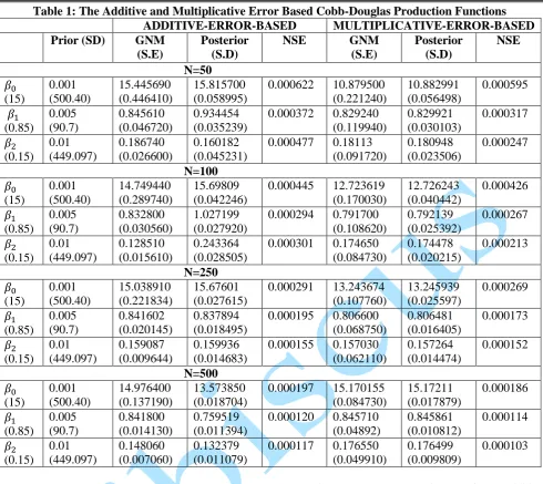
Table 1: The Additive and Multiplicative Error Based Cobb-Douglas Production Functions
ADDITIVE-ERROR-BASED MULTIPLICATIVE-ERROR-BASED
Prior (SD) GNM (S.E)
Posterior (S.D)
NSE GNM
(S.E) Posterior (S.D) NSE N=50 𝛽0 (15) 0.001 (500.40) 15.445690 (0.446410) 15.815700 (0.058995)
0.000622 10.879500 (0.221240) 10.882991 (0.056498) 0.000595 𝛽1 (0.85) 0.005 (90.7) 0.845610 (0.046720) 0.934454 (0.035239)
0.000372 0.829240 (0.119940) 0.829921 (0.030103) 0.000317 𝛽2 (0.15) 0.01 (449.097) 0.186740 (0.026600) 0.160182 (0.045231)
0.000477 0.18113 (0.091720) 0.180948 (0.023506) 0.000247 N=100 𝛽0 (15) 0.001 (500.40) 14.749440 (0.289740) 15.69809 (0.042246)
0.000445 12.723619 (0.170030) 12.726243 (0.040442) 0.000426 𝛽1 (0.85) 0.005 (90.7) 0.832800 (0.030560) 1.027199 (0.027920)
0.000294 0.791700 (0.108620) 0.792139 (0.025392) 0.000267 𝛽2 (0.15) 0.01 (449.097) 0.128510 (0.015610) 0.243364 (0.028505)
0.000301 0.174650 (0.084730) 0.174478 (0.020215) 0.000213 N=250 𝛽0 (15) 0.001 (500.40) 15.038910 (0.221834) 15.67601 (0.027615)
0.000291 13.243674 (0.107760) 13.245939 (0.025597) 0.000269 𝛽1 (0.85) 0.005 (90.7) 0.841602 (0.020145) 0.837894 (0.018495)
0.000195 0.806600 (0.068750) 0.806481 (0.016405) 0.000173 𝛽2 (0.15) 0.01 (449.097) 0.159087 (0.009644) 0.159936 (0.014683)
0.000155 0.157030 (0.062110) 0.157264 (0.014474) 0.000152 N=500 𝛽0 (15) 0.001 (500.40) 14.976400 (0.137190) 13.573850 (0.018704)
0.000197 15.170155 (0.084730) 15.17211 (0.017879) 0.000186 𝛽1 (0.85) 0.005 (90.7) 0.841800 (0.014130) 0.759519 (0.011394)
0.000120 0.845710 (0.04892) 0.845861 (0.010812) 0.000114 𝛽2 (0.15) 0.01 (449.097) 0.148060 (0.007060) 0.132379 (0.011079)
0.000117 0.176550 (0.049910)
0.176499 (0.009809)
0.000103
5. FINDINGS AND DISCUSSIONS
Table shows the estimates obtained using the Cobb-Douglas production function with additive error and multiplicative error term. The priors used are 0.001 (500.40), 0.005 (90.7), 0.01 (449.097) under the various sample sizes of study with the standard errors (SD) in bracket, a metropolis Hasting Within Gibbs algorithm was used with the Normal-Gamma prior to obtain the posterior estimates as recorded above using the additive and multiplicative error models. The result shows that the multiplicative error model behaves better than the additive error model.
Furthermore, the nuisance parameter 𝛽0shows a fluctuated and unsteady behaviour by producing values that are close to the true values for additive error model using the Gauss-Newton method while the estimates are far from the true values as sample size increased for the multiplicative error model. The estimates obtained by the Bayesian method are also closer to the true parameter values for the additive model than for the multiplicative model. In
general, the parameter estimates from additive model are better than those produced by the multiplicative model for both classical and Bayesian approaches.
Lastly, the standard error of the GNM and the Numerical Standard Error of the posterior decrease consistently as sample size increases, however, the standard errors of the Bayesian approach are generally better than those of the classical approach.
6. CONCLUSION
Bayesian approached is preferred in using the Cobb-Douglas production function based on the minimal numerical standard errors produced in between the two approaches under investigation. The level of efficiency in the Bayesian estimation as sample size increases is shown as the numerical standard errors decreased with increase in sample sizes.
REFERENCES
[Ant09] Antony J. - A dual elasticity of substitution production function with an application to cross-country inequality. Economics Letters, 102, 10-12, 2009.
[Bal96] Baltagi B. H. - Econometrics Analysis of Panel Data, John Wiley, New York, NY, 1996.
[Bha93] Bhatti M. I. - Efficient estimation of random coefficient models based on survey data. Journal of Quantitative Economics, 9(1), 99-110, 1993.
[Bha97] Bhatti M. I. - A UMP invariant test for testing block effects: an example. Far East Journal of Theoretical Statistics, 1(1), 39-50, 1997.
[BO96] Bhatti M. I., Owen D. - An econometrics analysis of agricultural performance in Sichuan, China. Asian Profile, 26(6), 443-57, 1996.
[BW88] Berger J. O., Wolpert R. L. - The
Likelihood Principle: A Review,
Generalizations, and Statistical
Implications. Hayward Institute of Mathematical Statistics, 1998.
[BKC98] Bhatti M. I., Khan I. H., Czerkawski C. - Agricultural productivity in
Shanghai region of China: an
econometric analysis. Journal of Economic Sciences, 1(2), 1-12, 1998.
[Chr01] Christensen R. - Advance Linear Modelling, 2nd ed., Springer, New York, 2001.
[CD28] Cobb C. W., Douglas P. H. - A Theory of Production, American Economic Review pp. 139 – 165, 1928.
[GQ73] Goldfield S. M., Quandt R. E. -
Nonlinear Methods of Econometrics,
North-Holland publication Company, Amsterdam, New York, 1973.
[Hoq91] Hoque I. - An application and test of
random coefficient model in
Bangladesh agriculture. Journal of Applied Econometrics, 6, 77-9, 1991.
[Hou55] Houthakker H. S. - The Pareto Distribution and the Cobb-Douglas Production Function in Activity Analysis, Review of Economic Studies, 23, 27-31, 1955.
[HA10] Hossain Z., Al-Amri K. S. - Use of Cobb-Douglas production model on some selected manufacturing industries in Oman. Education, Business and Society: Contemporary Middle Eastern Issues, 3(2), 78–85, 2010. doi:10.1108/17537981011047925
[HH07] Hájková D., Hurník J. - Cobb-Douglas Production Function: The Case of a Converging Economy. Czech Journal of Economics and Finance 57, 465-476, 2007.
[HM15] Hossain M., Majumder A. K. - On Measurement of Efficiency of Cobb-Douglas Production Function with Additive and Multiplicative Errors. Stat., Optim. Inf. Comput., Vol. 3, pp 96–104, 2015.
[HBA04] Hossain Z., Bhatti I., Ali Z. - An econometric analysis of some major manufacturing industries: A case study. Managerial Auditing Journal, 19(6),
790 – 795, 2004.
doi:10.1108/02686900410543895
[IL99] Ingene C. A., Lusch R. F. - Estimation of a department store production function. International Journal of Physical, Distribution & Logistics Management, 29, 453-64, 1999.
[Jon05] Jones C. I. - The Shape of Production
Functions and the Direction of
Technical Change, Quarterly Journal of Economics, 120, 517-549, 2005.
[Mok02] Mok V. W. K. - Industrial productivity in China: the case of the food industry in Guangdong province. Journal of Economic Studies, 29, 423-31, 2002.
[Pra08] Prajneshu - Fitting of Cobb-Douglas production functions: revisited. Agricultural Economics Research Review, 21, 289-92, 2008.
[Roy97] Royall R. - Statistical Evidence A Likelihood Paradigm. Chapman and Hall/CRC, Boca Raton, 1997.
[Sol56] Solow R. M. - A Contribution to the Theory of Economic Growth, Quarterly Journal of Economics 70, 65-94, 1956.