Collaboration-Type Identification in Educational Datasets

Collaboration-Type Identification in

Educational Datasets

ANDREW E. WATERS Department of Electrical and Computer Engineering Rice University

[email protected]

CHRISTOPH STUDER School of Electrical

and Computer Engineering Cornell University

[email protected]

RICHARD G. BARANIUK

Department of Electrical and Computer Engineering Rice University

[email protected]

Identifying collaboration between learners in a course is an important challenge in education for two reasons: First, depending on the courses’ rules, collaboration can be considered a form of cheating. Second, it helps one to more accurately evaluate each learner’s competence. While such collaboration identification is already challenging in traditional classroom settings consisting of a small number of learners, the problem is greatly exacerbated in the context of both online courses or massively open online courses (MOOCs) where potentially thousands of learners have little or no contact with the course instructor. In this work, we propose a novel methodology for collaboration-type identification, which bothidentifieslearners who are likely collaborating and alsoclassifiesthe type of collaboration employed. Under a fully Bayesian setting, we infer the probability of learners’ succeeding on a series of test items solely based on graded response data. We then use this information to jointly compute the likelihood that two learners were collaborating and what collaboration model (or type) was used. We demonstrate the efficacy of the proposed methods on both synthetic and real-world educational data; for the latter, the proposed methods find strong evidence of collaboration among learners in two non-collaborative take-home exams.

1 I

1.1 TODAY’S CHALLENGES IN IDENTIFYING COLLABORATION

learner’s true level of competence. If, for example, a group of learners work together on a set of homework problems, then it is difficult to evaluate the competence of each individual learner as opposed to the competence of the group as a whole. This aspect is especially important in scenarios where learners are simply copying the responses of a single peer. In such a scenario, a series of correct answers among collaborative group members could lead to the conclusion that all learners have mastered the material when—in reality—only one learner in the group achieved proficiency.

Manually identifying collaboration among learners is difficult enough when the class size is moderately small, say20–30learners, where an instructor may have a reasonable knowledge

about the aptitudes and habits of each particular learner. The problem is exacerbated as the class size increases to university-level classes with hundreds of learners. In the setting of online education, such as massive open online courses (MOOCs), a manual identification of learner collaboration (or cheating-through-collaboration) becomes infeasible, as potentially thousands of learners may be enrolled in a course, without ever having face-to-face interaction with an instructor (Pappano, 2012).

1.2 AUTOMATED COLLABORATION IDENTIFICATION

An alternative to manually identifying learners that collaborate is to rely on statistical methods that sift through learner response data automatically. Such data-driven methods look for pat-terns in learner answer data in order to identify potential collaborations. A naïve approach for automated identification of collaboration in educational datasets, such as multiple-choice tests, would consist of simply comparing the answer patterns between all pairs of learners and flag-ging learner pairs that exhibit a high degree of similarity. This approach, however, is prone to fail, as it ignores the aptitude of the individual learners, as well as the intrinsic difficulty of each test item or question (Levine and Donald, 1979; Wesolowsky, 2000).

In order to improve on such a naïve approach, a wealth of prior work exists on developing statistically principled methods of collaboration detection. Many of these methods focus on detecting the case of simple answer copying and a variety of statistical tests have been derived for this use case (Wollack, 2003; Sotaridona and Meijer, 2002; Sotaridona and Meijer, 2003; Wesolowsky, 2000). The proposed methods typically involve two steps: First, they estimate the probability that each learner will provide the correct response to each question by fitting models to both learners and questions. Second, they examine the actual answers provided by learners and compute a statistical measure on how likely the learner response patterns are to have arisen by chance. While such methods for collaboration identification have led to promising results, they possess a number of limitations:

data.

• The second limitation is in the explanatory weakness of the methods used in the existing col-laboration identification literature for predicting the success of each learner on each question. Learning analytics (LA) is concerned with jointly estimating learner ability and question dif-ficulty and using these estimates to predict future observations. More advanced LA methods have the potential to further improve the performance of automated collaboration identifica-tion.

• The third limitation is the use of simplistic models for how collaborative behavior between learners manifests in learner response data. Concretely, these methods are primarily con-cerned with the case of one learner copying the answers of another learner. The method of (Wesolowsky, 2000), for example, proposed the combination of point-estimates of the learner’s success probability (which are estimated directly from multiple-choice test results) and a basic model on the number of correspondences that should arise between learners based on these success probabilities. However, this method does not take into account the variety of complex ways that learners could collaborate, ranging from simple copying to symbiotic collaboration. By employing a variety of models for different types of collaborative scenar-ios, one could hope to improve overall identification performance as well as provide valuable information to educators.

1.3 CONTRIBUTIONS

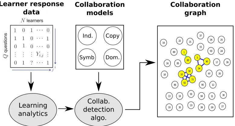
This paper develops a novel methodology for collaboration-type identification, which jointly identifies which learners engaged in collaboration and classifies the type of collaboration em-ployed. A block diagram of our methodology is shown in Figure 1. Our approach overcomes the limitations of existing approaches described in Section 1.2. Concretely, we make the following four contributions, each one corresponding to one of the four blocks shown in Figure 1.

• Generic learner response data: Our methodology relies only on simple right/wrong response data as opposed to multiple-choice responses (which usually contain multiple options per question). This response model enables our approach to be applied to a much broader range of educational datasets than existing methods.

Ind. Copy

Dom. Symb

Learning analytics

Collab. detection

algo.

1

88 5

34 90

10

62 73 92

11 12

13 14

15

16 17

18 19

20 21

22

23

24 25 26

27 28 29

30

33 35

37

39 85

86

87 89

91 93

94 95

Learner response

data Collaborationmodels

Collaboration graph

Figure 1: Block diagram for our proposed methodology for collaboration-type identification. The methodology consists of (i) learning analytics (Section 2) that model the success proba-bilities between learners and questions from learner response data, (ii) collaboration models

(Section 3) for various types of real-world collaborative behavior, and (iii)collaboration detec-tion algorithms(Section 4) that jointly identify collaboration and classify it according to one of the collaboration models. Thecollaboration graphsummarizes the result of the collaboration detection algorithm graphically. In this example, the collaboration graph depicts collaboration on a final exam for an undergraduate electrical engineering course. Collaboration was detected among three groups of learners. In two cases, collaboration is classified as symbiotic (denoted by solid, dark blue lines). In the other case, collaboration was classified as parasitic copying (denoted by the dashed, green line). Further details of this real-world application example are given in Section 5.

• Improved models for collaboration type: Our methodology proposes four novel models for describing collaboration in real-world educational scenarios. By employing these models, our methodology provides superior performance and increased flexibility in representing real-world collaborative behavior.

• Novel algorithms for collaboration-type identification: Our methodology provides two novel algorithms for collaboration-type identification that fuse LA and collaboration models. These algorithms have superior performance compared to state-of-the-art algorithms for detecting collaboration in educational datasets.

1.4 ORGANIZATION OF THE PAPER

of collaborative behavior between pairs of learners. In Section 4, we develop two novel algo-rithms for collaboration-type identification that make direct use of LA and collaboration models to search for likely pairs of learners engaged in collaboration. To demonstrate the efficacy of the proposed methodology, we validate our algorithms on both synthetic and real-world educational data in Section 5. We conclude in Section 6. The computational details of our methods are relegated to Appendices A, B, and C.

2 S

L

A

As discussed above, naïve methods for collaboration identification that simply compare the pat-tern of right/wrong learner responses are prone to fail because they do not take into account the ability of each learner and the difficulty of each question. We use the termlearning analytics

(LA) to refer to methods that estimate the probability that a given learner will be successful on a given question. LA is typically accomplished by specifying models on both the learner abilities and the question difficulties. By fusing these, one can formulate a statistical model and develop corresponding algorithms for estimating the success probability of a given learner for each question. Recent approaches to LA enable us to distinguish scenarios where two learners have highly similar response patterns due to active collaboration as opposed to simply having similar abilities or a set of very easy/hard questions, where learners jointly succeed/fail with high probability.

The collaboration identification methodology developed in this work is generic in that one may use an arbitrary LA algorithm. In this section, we briefly summarize two of our preferred approaches to LA, namely Bayesian Rasch and SPARFA. We will assume that the datasets con-sist of learner response data forN learners andQ questions. These questions can be adminis-tered in a variety of settings, such as during an exam or as a series of homework problems. For the sake of simplicity of exposition, we further assume that our data is fully observed; that is, each learner responds to every question. Extending our methods to the case of partially observed data is straightforward.

2.1 BAYESIAN RASCH LEARNING ANALYTICS

The Rasch model (Rasch, 1960; Rasch, 1993) is a simple, yet powerful approach to LA. This model assumes that each learner can be adequately characterized by a single latent ability pa-rameter, ci ∈ R, i = 1, . . . , N. Large positive values of ci indicate strong abilities, while

large negative values indicate weak ability. Questions are also modeled by a single parameter µj ∈ R, j = 1, . . . , Q, with large positive values indicating easy questions and large negative

values indicating difficult questions. By defining the slack variables

Zi,j =ci +µj, ∀i, j,

the Rasch model expresses the probability of userianswering questionj correctly (withYi,j = 1) or incorrectly (withYi,j = 0) using

Yi,j ∼Ber Φ(Zi,j)

, _∀i, j.

Here,Ber(x)denotes a Bernoulli distribution with meanx, while the function Φdenotes a link

model deploys the inverse logistic link function defined as

Φlog(x) = exp(x)

1 + exp(x).

Alternatively, one can use the inverseprobitlink function defined as

Φpro(x) =

Z x

−∞ 1

√

2πexp(−t

2_/2)dt.

An advantage of the inverse probit link function (over the inverse logistic link) is that, when coupled with suitable prior probability distributions (i.e., Gaussian distributions) for each pa-rameter, it enables efficient Markov chain Monte–Carlo (MCMC) methods based on Gibbs’ sampling (Gelman et al., 1995). In what follows, we exclusively make use the inverse probit link function and use the simplified notationΦ(x) = Φpro(x).

MCMC methods enable us to sample from the posterior distribution of each Rasch param-eter of interest in a computationally tractable manner. Among these paramparam-eters is the latent success probabilitypi,j = Φ(Zi,j), which denotes the probability of userj correctly responding

to questioni. Such a Rasch MCMC sampler will produce a series of samples from the posterior distribution ofpi,j that will be useful when developing the collaboration-type detection

algo-rithms in Section 4. We reserve the treatment of the full sampling details of the Rasch MCMC sampler for Appendix A.

2.2 SPARSE FACTOR ANALYSIS(SPARFA) LEARNING ANALYTICS

Like the Rasch model, SPARFA (Lan et al., 2013) characterizes the success probability of a set of learners across multiple questions. In contrast, however, the SPARFA model assumes that there are K latent factors, referred to as concepts, that govern the learners’ responses to these questions. In particular, SPARFA deploys the following model for the graded right/wrong response data:

Yi,j ∼Ber(Φ(Zi,j)) with Zi,j =wTi cj+µi, ∀i, j. (1)

Here, the vector cj ∈ RK, j = 1, . . . , N, represents the concept mastery of the jth learner,

with itskth entry representing the learner’s mastery of conceptk. The vectorwi ∈ RK models

theconcept associations, i.e., encodes how questioniis related to each concept. The scalar µi

models theintrinsic difficulty of questioni, where positive large values indicate easy questions (as in the Rasch model).

Retrieving the parameterscj,wi, andµi from the set of graded learner responsesYi,j in (1)

is, in general, an ill-posed inverse problem. To enable tractable inference, SPARFA assumes that the number of conceptsK is small compared to both the number of learners and questions, i.e.,K N, Q. Furthermore, to both enable interpretability and alleviate problems with model identifiability, SPARFA imposes non-negativity and sparsity on the question–concept vectors wi. These assumptions are imposed on the SPARFA model through the selection of the prior

distributions for each parameter of interest.

The SPARFA MCMC sampler extracts samples from the posterior distribution of each pa-rameter of interest, with the primary concern for collaboration detection being the samples of pi,j = Φ(Zi,j). As with the Rasch approach, we reserve the treatment of the full sampling details

3 S

-

Learners in real-world educational settings typically use a variety of strategies for providing responses to questions. In many cases, learners simply work independently (i.e., without any collaboration). In other cases, weaker learners may simply copy the responses of a stronger classmate. In yet other cases, learners may work together collaboratively such that every learner within the group both participates and benefits. Learners may also defer to one trusted learner’s answer, regardless of whether or not the trusted learner is actually correct. The fact that learn-ers may collaborate on only a subset of questions further complicates automated collaboration identification.

By explicitly modeling collaboration type, one could hope to both provide valuable infor-mation regarding collaboration as well as to improve detection of collaborating learners. To this end, we propose four statistical collaboration models that capture a range of different scenarios. We use the notation Mm for m = 1, . . . ,4 to refer to each model. We express our models

probabilistically for a given pair of learners, i.e., learner u and learnerv, and model the joint probability distribution of observing the set of answers(Yi,u, Yi,v). This joint distribution

natu-rally depends first on the prior success probabilities pi,u andpi,v of both learners. In practice,

these probabilities can be estimated via an LA approach such as the Bayesian Rasch model (see Section 2.1) or SPARFA (see Section 2.2). All models (with the exception of the independence model) are parameterized by a scalar variableε1 ∈[0,1], which characterizes the probability that two learners will choose to collaborate on a given question. This parametrization enables us to capture the fact that learners might only collaborate on a subset of allQquestions. Additionally, two of the collaboration-type models we propose will utilize a second parameter, ε2 ∈ [0,1]; the meaning of this parameter is model specific and will be explained when applicable. To sim-plify notation, we will use the following definitionsε¯1 = 1−ε1 and ε¯2 = 1−ε2, as well as

¯

pi,u = 1−pi,uandp¯i,v = 1−pi,v.

3.1 COLLABORATIVE MODELS

INDEPENDENCE MODEL_M1 Under the independence model, a pair of learners is not collab-orating. Instead, each learner answers the assigned questions independently. Hence, there are no parametersεfor this model. The probability of observing any answer sequence for two learners working independently is simply given by the product of the individual prior probabilities. For example, the graded response pair(1,0)is achieved if learner uprovides a correct response to theith question, while learner v provides an incorrect response. This case occurs with proba-bilitypi,up¯i,v. The likelihoods for each of the four possible observed set of responses under the

independence model for a given question are given in Table 1.

Table 1: Independence modelM1

Yi,u Yi,v P(Yi,u, Yi,v|pi,u, pi,v, ε1, ε2)

0 0 p¯i,up¯i,v 0 1 p¯i,upi,v 1 0 pi,up¯i,v 1 1 pi,upi,v

Table 2: Parasitic modelM2

Yi,u Yi,v P(Yi,u, Yi,v|pi,u, pi,v, ε1, ε2)

0 0 p¯i,up¯i,vε¯1+ε1(¯pi,uε¯2 + ¯pi,uε2)

0 1 p¯i,upi,vε¯1

1 0 pi,up¯i,vε¯1

1 1 pi,upi,vε¯1+ε1(pi,uε¯2 +pi,uε2)

Table 3: Dominance modelM3

Yi,u Yi,v P(Yi,u, Yi,v|pi,u, pi,v, ε1, ε2)

0 0 p¯i,up¯i,v+ ¯pi,upi,vε1ε2+pi,up¯i,vε1ε¯2

0 1 p¯i,upi,vε¯1

1 0 pi,up¯i,vε¯1

1 1 pi,upi,v+ ¯pi,upi,vε1ε¯2+pi,up¯i,vε1ε2

Table 4: OR modelM4

Yi,u Yi,v P(Yi,u, Yi,v|pi,u, pi,v, ε1, ε2)

0 0 p¯i,up¯i,v 0 1 p¯i,upi,vε¯1

1 0 pi,up¯i,vε¯1

1 1 pi,upi,v+ ¯pi,upi,vε1+pi,up¯i,vε1

in the event that (i) both learners do not collaborate on the question and both provide incor-rect responses independently or (ii) both learners are collaborating on the question and that the learner chosen to solve the question does so incorrectly. The probability of this event is given byp¯i,up¯i,vε¯1+ε1(¯pi,uε¯2+ ¯pi,uε2). The likelihood table for each of the four possible observed set of responses under the parasitic model is given in Table 2.

DOMINANCE MODEL M3 Under the dominance model, each learner works a question inde-pendently, after which each pair of learners discusses which of the two answers will be used. Un-der this model, each of the two learners attempts to convince the other to accept their response. The parameterε1denotes the probability that the pair will collaborate on a given question (anal-ogous to the parasitic model), while the second parameterε2denotes the probability that learner uwill convince learner v to adopt their response. For example, ε2 = 1implies that learneru will always convince learnerv, whileε2 = 0indicates the opposite scenario. Under this model, observing the graded response pair(0,0)occurs in either the event that (i) both learners get the

incorrect response (regardless of which learner dominates) or (ii) only one learner produces an incorrect responses, but convinces the other learner to accept the response. The probability of this event is given byp¯i,up¯i,v + ¯pi,upi,vε1ε2 +pi,up¯i,vε1ε¯2. The likelihood table for each of the four possible observed set of responses under the dominance model is given in Table 3.

OR MODEL _M4 Under the OR model, each learner may not be able to provide the correct response to a given question. However, they can identify the correct response if at least one of them is able to provide it. Thus, the learner pair will jointly provide the correct response if at least one of the learners succeeds. The name of this model derives from the Boolean OR function, which is1if either one or both inputs to the function are1and0otherwise. This model

they are collaborating on the question) or (ii) only one learner produces the correct response and the pair is actively collaborating on the given question. This probability of this scenario is given bypi,upi,v+ ¯pi,upi,vε1+pi,up¯i,vε1. The likelihood table for each of the four possible observed sets of responses under the OR model for questioniis given in Table 4.

3.2 DISCUSSION OF PAIRWISE COLLABORATION MODELS

Many more models can be developed to emulate various collaboration types. Such new models can be easily integrated into our methodology. We further note a number of correspondences that exist between the collaboration models detailed above. For example, the modelsM2,M3, andM4are equivalent toM1 wheneverε1 = 0, i.e., with the collaboration probability equal to zero. Further, modelsM2 andM4 are equivalent under the same value of ε1 and wheneverε2 is either0or1.

One limitation of the collaboration models proposed above is that we have entirely decoupled the collaboration rate parameterε1from the success probabilitiespi,uandpi,v. In real educational

scenarios, learners might choose to collaborate when they perceive a large potential benefit. Learners may, for example, be less likely to collaborate on questions that they are likely to answer correctly (i.e.,pi,u, pi,v are large) and more likely to collaborate on questions that they

are likely to answer incorrectly (i.e.,pi,u, pi,v are small). The development of such collaboration

models is an interesting topic for future work.

4 A

C

-T

I

We now develop two novel algorithms for pairwise collaboration-type identification. Both al-gorithms jointly utilize learner–response data, an LA method, and a set of collaboration models to jointly detect and classify different types of collaboration in educational datasets (recall Fig-ure 1).

The first algorithm, referred to as sequential hypothesis testing(SHT), uses a Bayesian hy-pothesis test first introduced in (Waters et al., 2013). This algorithm examines the joint answer sequence of a pair of learners and evaluates the likelihood that such patterns would arise inde-pendently (under modelM1) or under one of the other collaboration model (M2,M3, orM4). The second algorithm, referred to ascollaborative model selection(CMS), uses Bayesian model selection (Hoff, 2009) in order to jointlycompute posterior distributions on the probability of learner response data arising under various collaboration models.

4.1 SEQUENCE HYPOTHESIS TESTING (SHT)

SHT compares two hypotheses. The first hypothesisH1 corresponds to the case where learner u andv collaborate under a pre-defined collaboration-type model Mm, m 6= 1, given the LA

parameters. The second hypothesisH2of SHT assumes that the number of agreements between the graded responses of learneru andv are a result of the independence model_M1, given the LA parameters.

4.1.1 Collaboration hypothesis

Mm, m 6= 1. Note that the SHT method can be utilized with any of the collaborative models

introduced in Section 3. The model proposed here relies on the individual probabilities pi,u

andpi,v, which are the probabilities of learner u and v succeeding in questioni given the LA

parameters. For ease of exposition, we will proceed with our derivation for a two-parameter model such asM2 orM3 with parametersε1 andε2; the reduction to a single parameter model (such as the OR model) or the extension to a model with additional parameters is straightforward. Assuming uniform priors onε1 andε2over the range[0,1]our collaboration hypothesis for a given modelMmis simply given by

P(H1| Mm) =

Z 1

0

Z 1

0

Q

Y

i=1

P(Yi,u, Yi,v|pi,u, pi,v, ε1, ε2,Mm)dε1dε2, (2)

which corresponds to the probability of observing the pair of sequences of graded responses for allQ questions under the collaboration model_Mm. The quantity in (2) can be computed

efficiently via convolution; we reserve the computation details for Appendix C.

4.1.2 Independence hypothesis

The probability of the second hypothesis H2 for SHT corresponds to the probability of the observed pair of graded response sequences, given the success probabilitiespi,uandpi,vobtained

under the independence modelM1, i.e.,

P(_H2) =

Q

Y

i=1 pYi,u

i,u p¯

(1−Yi,u)

i,u p Yi,v

i,v p¯

(1−Yi,v)

i,v . (3)

Given the probabilities (2) and (3) for the hypothesesH1andH2, respectively, we can finally compute thelog Bayes factor1_{for SHT for a given pair of learners as follows:}

LBF= log

P(H1) P(_H2)

. (4)

A log Bayes factor greater than 0indicates more evidence for the collaborative hypothesis

(under the chosen modelMm) than the independent hypothesis, while a log Bayes factor smaller

than0indicates the reverse scenario. In general, however, a large value of the log Bayes factor

is required when asserting that the evidence of collaboration is strong.

4.1.3 Discussion of SHT

The primary advantage of the SHT method is computational efficiency and flexibility. It can be used with simple point estimates of the learner success probabilities. Thus, it can be eas-ily incorporated into classical approaches for LA, such as the standard (non-Bayesian) Rasch model (Rasch, 1993) or item-response theory (IRT) (Bergner et al., 2012). When utilized in this way, the log Bayes factor needs only be computed once for each pair of students, making it computationally very efficient.

SHT can also be used with a fully Bayesian LA approach (such as those detailed in Section 2 that provide full posterior distributions of the learner success probabilities). This is done by

1_{Under a uniform prior, the log Bayes factor is called the log likelihood ratio (LLR) in the statistical signal}

Figure 2: Graphical model for collaborative model selection (CMS).

adding the computation of(4)as an additional sampling step of the MCMC sampler. Concretely,

we compute (4) at each iteration of the MCMC sampler given the current estimates of pi,u

andpi,v, ∀i, u, v. The log Bayes factor can be equivalently converted to a posterior probability

for each hypothesis, from which we can sample the hypotheses directly as part of the MCMC sampler. This approach has the advantage of improving the robustness of our inference over classical approaches, albeit at higher computational cost.

One restriction of our method is that SHT compares the independence model M1 against exactly one other collaboration model Mm. One could, however, consider testing multiple

models simultaneously by using a form of Bonferroni correction to control the family-wise error rate (Westfall et al., 1997). The approach proposed in the next section avoids such necessary corrections by means of Bayesian model selection.

4.2 FULLYBAYESIAN COLLABORATIVE MODELSELECTION

We now turn to a collaboration-type indentification method based on Bayesian model selection (Hoff, 2009). This method allows us tojointlyexplore multiple collaboration models (types) and to extract the associated model parameters in an efficient way in order to find configurations that best explain the observed data. The result will provide estimates of the full posterior distributions for each collaboration model and each parameter of interest. We dub this methodcollaborative model selection(CMS).

4.2.1 Generative model for CMS

We first present the complete generative model for the pairwise collaborative model and state all necessary prior distributions. This will enable efficient MCMC sampling methods for estimating the relevant posterior distributions.

The full generative model is illustrated in Figure 2 for the case of the SPARFA LA model (the equivalent Rasch-based model is obtained by removing the nodeWand replacingCwith the vectorc). By symmetry of the proposed collaboration models, collaboration between each pair of N learners can be specified with D = (N2−N)/2 total models and corresponding

sets of the associated model parameters. We will use the quantity Md to denote the random

variable that indexes the collaboration model for learner pair d; the notation εd denotes the

random vector of model parameters for learner paird. For the collaborative model index Md

we assume a discrete prior πm,d such that P4_m=1πm,d = 1 for all d. For the elements of the

parameter vectorεd, we assume a Beta-distributed priorBeta(αε, βε). Generation of the latent

model parametersεd.

4.2.2 MCMC sampling for collaboration type detection

Given the graded response data matrixYalong with the prior distribution onMdandεd, we wish

to estimate the posterior distribution of each model index along with its respective parameters for each pair of learners d = 1, . . . , D. Doing this will allow us to infer (i) which pairs of learners are collaborating, (ii) what type of collaborative model are they using, and (iii) how strong the evidence is for these assertions.

We use Bayesian model selection techniques (Hoff, 2009) to efficiently search the space of possible models and model parameters for configurations that best explain the observed data Y. Full conditional posteriors for the models and model parameters, however, are not avail-able in closed form, rendering Gibbs’ sampling infeasible. Thus, we make use of a suitavail-able Metropolis-Hastings step (Gelman et al., 1995). Specifically, assume that at iterationt of the MCMC sampler and for a specific pair of learnersd, we have a model sampleMt

dparametrized

byεt

d. The Metropolis-Hastings step proceeds by proposing a new modelMdt+1with parameters

ε_dt+1via some proposal distributionq(M_dt+1,εt_d+1|Mt

d,εtd). We will utilize a proposal distribution

of the following form:

q(M_it+1,εt_i+1_|M_it,εt_i) = qε(εt_i+1_|M_it+1, M_it,εt_i)qM(Mit+1|Mit,εti) =qε(εt_i+1_|M_it+1, M_it,εt_i)qM(Mit+1|Mit).

In words, we (i) split the proposal into a model component and model parameters component and (ii) make use of a proposal for the modelMdthat is independent of the model parametersεd.

We implement this proposal in two steps: First, we proposeM_dt+1 _∼ qM(M_dt+1|Mdt). Note that

there are many choices for this proposal; we will make use of the following simple one given by

p(M_dt+1 =Mt+1_|Mt

d=Mt) =

(

γ, ifMt+1 _=Mt

1−γ

|M|−1, ifM

t+1 _6=Mt_. (5)

Here, γ ∈ (0,1) is a user-defined tuning parameter. In words, with probabilityγ the MCMC sampler will retain the previous model; otherwise, one from the remaining|M| −1models is

proposed uniformly. The proposal for the parametersεt_d+1 takes the following form:

q(εt_d+1_|M_dt+1, M_dt,εt_d) =

    

δ0, ifMdt+1 =M1

qβ(εtd+1|Mdt+1, Mdt,εtd), ifMdt+1 =Mt,

πε(ε|αε, βε), otherwise,

(6)

where δ0 corresponds to a point-mass at 0; the distribution qβ corresponds to a random walk

proposal on the interval[0,1]defined by

qβ(a|b) = Beta(cb, c(1−b)), (7)

wherec >0is a tuning parameter. In words, the sampling ofεt_d+1(i) is performed via a random

walk when the model remains unchanged, (ii) is drawn directly from the priorπε(ε|αε, βε)when

a new model non-independent model is proposed, and (iii) is set to0when the model changes

convenience). Note that it can be shown that the mean of the proposal distributionqβ is simply

b (the previous value used) while the variance is c_c22(₊b−_c+1b2), which tends to zero asb approaches either0or1.

After proposing the new model {M_dt+1,εt_d+1} via (5)–(7) we accept the proposal with a

probabilityras

r= min

1,p(Y|M

t+1

d ,εtd+1)π(Mdt+1)π(εtd+1|αε, βε)qε(εtd|Mdt, Mdt+1,εdt+1)qM(Mdt|Mdt+1))

p(Y_|Mt

d,εtd)π(Mdt)π(εtd|αε, βε)qε(ε t+1

d |M t+1

d , Mdt,εtd)qM(M t+1

d |Mdt))

.

The accept/reject decision is computed individually for each learner paird = 1, . . . , D.

4.2.3 Discussion of CMS

The primary advantage of CMS is that it can jointly search across all collaborative models for each pair of learners in the dataset. This comes at the price of additional computational com-plexity, as a new set of models and model parameters must be proposed at each iteration of the MCMC.

We note that while our fully Bayesian method for collaboration detection uses the success probability matrixΦ(Z)when exploring new collaboration models, those models donot

influ-encethe sampling ofZitself. This is due to the structure of the model we have proposed, asY separates the LA portion of the MCMC from the CMS portion. This assumption is similar to the work in (Wesolowsky, 2000) which computes success probabilities for each learner–question pair based only on the dataYregardless of the evidence of collaboration.

The model depicted in Figure 2 could be augmented in a way that enables us to propose a new posterior distribution forZ where the current belief about the collaborative models will influence our beliefs about learner ability. For example, such a model could be accomplished by proposing an additional latent variable for the answer that a learner would have provided had they not been in collaboration; this would enable us to automatically temper our beliefs about learner ability in the event that we believe that they are involved in collaboration. We will leave such an approach for future work.

5 E

We now validate the performance our proposed methodology. We first examine the identification capabilities using synthetic data with a known ground truth. Following this, we showcase the capabilities of our methods on several real-world educational datasets.

5.1 SYNTHETIC EXPERIMENTS

We first validate the performance of our methodology using synthetic test data using both the SHT and CMS algorithms. We furthermore compare against two other methods. The first is the state-of-the-art method collaboration identification method developed in (Wesolowsky, 2000), which was designed specifically for handling responses to multiple choice exams, where one is interested in the specific option chosen by the pair of learners. Since we are interested in detect-ing collaboration given only binary (right/wrong) graded responses, we need to first modify the method (Wesolowsky, 2000) accordingly. Concretely, we set their termvi indicating the number

of wrong options for questionito1, meaning that all wrong answers are treated equally. The

is theagreement hypothesis testingmethod proposed in (Waters et al., 2013), which we will call AHT for short. This method utilizes a Bayesian hypothesis test similar to SHT that compares the likelihood of the independence modelM1 relative to a simple collaboration model in which two learners choose to agree in their answer patterns with some arbitrary probabilityδ. We refer the interested reader to (Waters et al., 2013) for further details.

5.1.1 Performance metrics

In order to evaluate collaboration identification performance, we will examine how well the con-sidered methods identify learners who collaborate relative to learners who work independently. Each of the four methods naturally outputs acollaboration metricrelated to the probability of collaboration between each pair of learners:

• Bayesian Hypothesis Tests (AHT and SHT):For each learner pair, the collaboration metric is given by the log Bayes’ factor.

• Bayesian Model Selection (CMS):For each learner pair, we first threshold on the posterior probability that two learners worked under a collaborative model and then, we rank them ac-cording to the posterior mean ofε1.

• Wesolowsky’s Method: For each learner pair, the collaboration metric is given by theZ-score (see (Wesolowsky, 2000) for the details).

By sorting the output metrics in ascending order, a course instructor can easily see which pairs of learners in a class are most likely engaging in collaborative behavior. To this end, letξdenote the output vector of pairwise metrics for each learner pair for a given algorithm. Sorting the entries ofξ from smallest to largest, we can compute a normalized percentile ranking for each pair of learners. LetId denote the index of learner pairdin this sorted vector. The normalized

percentile ranking is then given simply by

Pd= I

d

D, d= 1, . . . , D, (8)

with larger values of Pd denoting higher likelihood of collaboration relative to the rest of the

entire learner population.

5.1.2 Algorithm comparison on synthetic data

As a first synthetic experiment, we consider a class ofN = 30learners (withD = 435unique

learner pairs) answering Q = 50 questions. Learner abilities are initially generated via the

SPARFA model. We select three pairs of learners who will work together collaboratively, one pair for each model M2, M3, and M4 as defined in Section 2. Each pair has a per-question collaboration probabilityε1 = 0.75, while the value forε2for each of the two-parameter models is set to0for simplicity. The answers for the collaborating learners are generated according the

0.75 0.8 0.85 0.9 0.95 1

ra

nk

in

g

pe

rf

or

m

an

ce

CMS SHT Wes. AHT

M₂ M₃ M₄ M₂ M₃ M₄ M₂ M₃M₄ M₂ M₃M₄

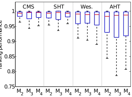
Figure 3: Normalized percentile ranking performance for all four collaboration methods with a synthetic dataset consisting of N = 30 learners and Q = 50 questions. Three learner pairs

are engaged in collaboration, one for each of the collaborative models, with a per-question collaboration probability ε1 = 0.75. Larger values indicate better identification performance. The CMS method achieves the best collaboration identification performance, followed by SHT, Wesolowsky’s method (denoted by “Wes.”), and AHT, respectively.

their answers are generated according to the SPARFA model via (1). We then deploy CMS, SHT, Wesolowsky’s method (denoted by “Wes.” in Figure 3), and AHT, and we compute the normalized percentile ranking for each learner pair according to (8). We repeat this experiment over 100 trials and present the normalized percentile ranking statistics for the collaborating

learner pairs for each collaboration model and each algorithm as a box-whisker plot.

From Figure 3, we see that CMS outperforms all other methods, both in the average and stan-dard deviation of the normalized percentile ranking. CMS is followed by SHT, Wesolowsky’s method, and AHT. Since our proposed CMS method shows the best collaboration identification performance, we focus exclusively on this method in the remaining synthetic experiments.

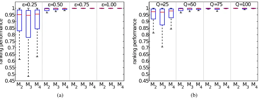
5.1.3 Performance evaluation for CMS over multiple parameters

We now examine the performance trends of the CMS method for a varying number of questions as well as the collaboration probability ε1. First, we generate data for N = 50 learners with Q= 50questions and sweep the collaboration probabilityε1 ∈ {0.25,0.5,0.75,1.0}and repeat this experiment over100trials. We again examine performance using the normalized percentile

ranking (8) and display the results in Figure 4(a). We can see that the performance is excellent for collaboration probabilities as low asε1 = 0.5, meaning that learners were expected to collab-orate on only every-other question. Second, we fixε1 = 0.5and sweepQ ∈ {25,50,75,100}. The result is displayed in Figure 4(b). We see that the proposed CMS method achieves excellent identification performance forQ≥50questions.

5.2 REAL-WORLD EXPERIMENTS

0.45 0.5 0.55 0.6 0.65 0.7 0.75 0.8 0.85 0.9 0.95 1 ra nk in g pe rf or m an ce

ε=0.25 ε=0.50 ε=0.75 ε=1.00

M₂ M₃ M₄ M₂ M₃ M₄ M₂ M₃ M₄ M₂ M₃M₄

(a) 0.45 0.5 0.55 0.6 0.65 0.7 0.75 0.8 0.85 0.9 0.95 1 ra nk in g pe rf or m an ce

Q=25 Q=50 Q=75 Q=100

M₂ M₃ M₄ M₂ M₃ M₄ M₂ M₃ M₄ M₂ M₃ M₄

(b)

Figure 4: Collaboration-type identification performance for the collaborative model selection (CMS) approach with a synthetic N = 50 learner dataset. (a) impact of varying

collabora-tion probabilitiesε1 ∈ {0.25,0.5,0.75,1.0} forQ = 50 questions; (b) impact of numbers of questions forQ_{∈ {}25,50,75,100_}with collaboration probabilityε1 = 0.5.

Tutor.2

5.2.1 Undergraduate signal processing course

We first identify collaboration on homework assignments in the course up to the first midterm examination. One interesting aspect of this course is that learners were encouraged to work to-gether on all homework assignments, albeit with some restrictions. Concretely, each learner was assigned into a group of2-to-4 learners with whom they were allowed to actively collaborate

on homework assignments. Learners within each group were free to discuss each homework problem as well as its solution with any members of their group, though each learner was re-quired to submit their own homework solutions for final grading. Learners were, however, not required to collaborate; the only restriction was that any collaboration with other learners was to be confined to the assigned homework group. Collaborating outside of the assigned homework group was considered cheating.

This particular setting presents an interesting test case for our method since we have a rough ground truth with which to compare our results. We examine the performance of CMS and the method of Wesolowsky on all homework assignments up to the first midterm exam; a total of Q = 50 questions andN = 38 learners. We further include all question–responses to the

midterm (14additional responses) in extracting the SPARFA parameters, though these questions

were excluded from the collaboration detection algorithm. The data is especially challenging since learners were given ample time to solve and discuss homework problems. Because of this, most responses given on homework problems were correct. As a consequence, an extremely high degree of similarity between answer patterns is required for collaboration to be considered probable.

For CMS we posit collaborative connections between learner pairs for whom Md 6= 1

(i.e., from which the independence model M1 is excluded) in more than 90% of MCMC

1

2 3

4 19

5 6

7 8 20

9

10 11

12 34

14

13

15 16 17

18

21

22

23 24 25 26

27

28

29 30 31 32

33 35

36

37 38

Figure 5: Collaboration-type identification result for the Bayesian model selection method for the first set of homework assignments in the undergraduate signal processing class dataset. The data consists of38learners answering50homework questions plus14midterm exam questions.

Grey ellipses designate the assigned homework groups. Dashed green lines denote parasitic collaborations, while solid blue lines denote symbiotic collaborations detected by CMS. Dotted red lines denote the connections found using Wesolowsky’s method, which, in general, finds fewer ground truth connections than the CMS method.

erations and for whom the posterior mean of ε1 was greater than 0.4. The Z-score threshold for Wesolowsky’s method was adjusted manually to provide the best match to the ground truth. We display the corresponding results in Figure 5. Dotted red lines denote connections detected under Wesolowsky’s method. For the Bayesian model selection method, blue solid lines denote detections under symbiotic (OR) model, whereas dashed green lines show detections under the parasitic model.

Most collaborative types found using CMS for this dataset are of the OR type. An exception is the group{9,10,12}, for which the parasitic copying model was proposed most frequently. Examination of the answer pattern for these learners show that while the joint answer patterns for these learners are very similar on the homework assignments, Learners10and12perform

homework is more a consequence of copying the responses of Learner9rather than because of

their mastery of the subject material. We additionally note the collaborative connection between Learners 9 and 24 as well as between Learners 10 and 14. These connections arise due to

high similarity in the homework answering patterns which are also quite different from the rest of the collaborative group. Interestingly, Wesolowsky’s method also found strong evidence of collaborations between Learners 9and 24; this method, however, failed to reveal three of the

intra-group collaborations found by our proposed CMS method. In the following, we omit further comparisons with Wesolowsky’s method for the sake of brevity.

As a second experiment with the same undergraduate signal processing course, we consider collaboration identification on the final exam, which was administered as a take-home test. Dur-ing this examination, learners were instructed not to collaborate or discuss their results with any other learners in the class. The final exam consisted of24questions. We deploy CMS

us-ing all questions in the course (a total of147questions) to extract the SPARFA parameters and

search for collaboration only on the questions on the final exam. We jointly threshold on the posterior mean ofε1 and the proportion of MCMC samples that indicated a non-independent collaborative model for each learner pair to arrive at the collaboration graph of Figure 6. We find strong evidence of collaboration between the learner pair{14,38}under the symbiotic col-laboration model. Interestingly, Learner14 was also detected in the previous experiment as a

learner working outside of his collaborative group on the course homework assignments. Both learners provided correct responses to each question on the final exam, although their previous performance in the course would lead one to expect otherwise. To prevent false accusations (see, e.g., (Chaffin, 1979) for a discussion on this matter), we examined their open form responses available in OpenStax Tutor and found a remarkable similarity in the text of their answers; this observation further strengthens our belief about their collaboration.

5.2.2 Final exam of an undergraduate computer engineering course

This course consists of97learners who completed the course answering a total of203questions,

distributed over various homework assignments and three exams. We examine collaboration among learners in the final exam, which consists of 38 questions. As was the case with the

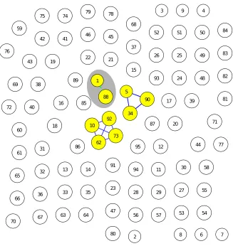
signal processing final exam, the computer engineering final exam was administered as a take-home examination where learners were instructed not to collaborate with their peers. In order to extract the SPARFA parameters, we use all questions administered during the entire course and then use CMS to extract the posterior distributions for each pair of learners on the subset of questions corresponding to the final exam. We jointly threshold the posterior probability of non-independent collaboration as well as the posterior mean of ε1. We display the result in Figure 7, where dashed green lines correspond to parasitic collaboration (M2) and solid blue lines denoting symbiotic collaboration (M4). Note that no collaborations were detected under the dominance model (M3).

All three groups of learners in Figure 7 for whom we identify collaboration have identical an-swer patterns. The group{10,92,62,73_}provides the correct response to every question on the

exam. The group{5,34,90}jointly miss only one question which is estimated by SPARFA to be in the mid to high range of difficulty. The group{1,88_}jointly miss the same two questions,

1

2

3

4

5

6

7 8 ₉

10

11 12

13

14

38

15 16

17

18 19

20

21

22

23 24

25

26 27

28 29

30

31

32 33

34

35 36

37

Figure 6: Collaboration-type identification result for a take-home exam in an undergraduate electrical engineering course consisting of38learners answering24questions. The connected

nodes correspond to learners for which the collaboration hypothesis. Manual inspection of the open-form responses provided by Learners14and 38further strengthens the collaboration

hy-pothesis.

group{10,62,73,92_}. This, coupled with the fact that each of the learners have only managed

to perform slightly better than what SPARFA would predict, allows us to reasonably exclude this group from further scrutiny. By contrast, the answer patterns for the other groups reveal strong evidence of collaboration due to very similar wording and grammar. This is especially true for the pair {1,88}; as it can be seen from Table 5, Learner 1 consistently provides a shortened version of the responses provided by Learner 88, including those answered incorrectly.3

6 C

We have developed new methods for pairwise collaboration-type identification in large educa-tional datasets, where the objective is to both identify which learners work together and classify the type of collaboration employed. Our framework combines sophisticated approaches to learn-ing analytics (LA) with new models for real-world collaboration and employs powerful algo-rithms that fuse the two to search for active collaborations among all pairs of learners. We have validated our methodology on both synthetic and real-world educational data and have shown

3_{We analyzed the same computer engineering dataset using a different collaboration detection framework in}

(Waters et al., 2013). We omitted two learners in this work due to their failure to submit all homework assignments. Thus, learner indices in these two papers differ. As an example, Learners1and88in this work thus correspond to

1 88 2 3 4 5 34 90 6 7 8 9 10 62 73 92 11 12 13 14 15 16 17 18 19 20 21 22 23 24 25 26 27 28 29 30 31 32 33 35 36 37 38 39 40 41 42 43 44 45 46 47 48 49 50 51 52 53 54 55 56 57 58 59 60 61 63 64 65 66 67 68 69 70 71 72 74 75 76 77 78 79 80 81 82 83 84 85 86 87 89 91 93 94 95

Figure 7: Collaboration identification result for a take-home exam in an undergraduate electrical engineering course consisting of 97 learners answering 38 questions. The connected nodes

correspond to learners identified by CMS to be collaborating, with dashed green lines denoting one-side copying and solid blue lines denoting symbiotic collaboration. Manual inspection of the open-form responses provided by Learners 1 and 88 (highlighted by a gray oval) reveals

Table 5: Selected responses of Learners 1 and 88 in the non-collaborative take-home exam. Answer similarities are highlighted in black. Both learners responded to the last item incorrectly.

Learner 1 Learner 88

double char integral double cannot be used to base a

switch decision int andcharcan be used as they are ofintegraltype

When thename field is defined. student.name would correctly

ac-cess the name field if the name of the student struct objectdeclaredis student.

A This prints the ASCII character

as-sociated with the decimal value 65, which isA

5 The value of x would be5; it would

truncate the digits right of the deci-mal point.

−2147483648−+2147483647 Its potential range is

−2,147,483,648− +2,147,483,647

(using the typical 32 bit representa-tion).

that they significantly outperform the state-of-the-art methods available in the open literature. Additionally, we detected several cases of non-permissible collaboration (which is considered cheating) on both homework assignments and examinations in two undergraduate-level courses. The collaboration rankings that our method provides can greatly facilitate collaboration iden-tification as it provides a good (and small) set of candidates that need to be evaluated in greater depth (with respect to collaborative behavior) by an instructor. This advantage reduces the in-structor’s workload and promotes fairness in educational settings.

One interesting avenue for future work involves modeling more complicated social groups among learners. In particular, extending the capability of collaboration detection methods be-yond pairwise collaboration is useful in real-world educational scenarios in which learners of-ten work in larger groups with complicated social dynamics. Another avenue for future work consists of using collaboration detection methods to “denoise” or, more colloquially, “decol-laborate” LA. Such an application is crucial in the deployment of intelligent tutoring systems (Nwana, 1990), as it could use its beliefs about collaboration to estimate the true learner ability (i.e., without collaboration).

arise when only the answer patterns themselves are considered.

A D

MCMC

B

R

-PROACH TO

L

A

Here, we derive the sampling steps for the Rasch MCMC sampler. Recall that the generative model for the dataY under the Rasch approach is given by

Yi,j ∼Ber(Φ(Zi,j)) with Zi,j =ci+µi, ∀i, j.

It can be shown (see, e.g., (Chib and Greenberg, 1998)) that this model is equivalent to

Yi,j ∼sign(Φ(Zi,j0 )) with Zi,j0 =ci+µi +ei,j, ∀i, j.

where sign(_·) is the signum function and ei,j ∼ N(0,1). This latter representation is more

convenient for the purposes of MCMC.

By specifying the following prior distributions

π(cj)_{∼ N}(0, σ_c2) and π(µi)_{∼ N}(0, σ_µ2),

we can perform Gibbs’ sampling on each of the variablescj, µj by augmenting with the latent

variableZ0

i,j. The sampling steps at each MCMC iteration are given by

(1) For alli = 1, . . . , Qandj = 1, . . . , N sampleZ0

i,j ∼ N(ci+µj,1), truncating above 0 if

Yi,j = 1, and truncating below 0 ifYi,j = 0.

(2) For alli= 1, . . . , Qsampleµi ∼ N(σeµ2

PN

j=1(Zi,j0 −cj),σeµ2), whereeσµ2 = σ12

µ +N

−1 .

(3) For allj = 1, . . . , N samplecj ∼ N(eσc2

PN

i=1(Zi,j0 −µi),eσ2c), whereσec2 = σ12

c +Q

−1 . By repeating this sampling scheme over several iterations, we assemble a set of samples from the posterior distribution of the Rasch parameterscj, ∀j andµi, ∀i. In addition, the values of

pi,j = Φ(cj +µi)are samples of the probability of learner j answering itemicorrectly, which

are then used by the collaboration-type identification algorithms of Section 4.

B D

MCMC S

SPARFA A

TO

L

A

Here, we discuss the sampling scheme for the SPARFA-based MCMC sampler. Like the Rasch MCMC sampler of Appendix A, we can introduce the latent variableZ0 _{and use the equivalent}

generative model

Yi,j ∼sign(Φ(Zi,j0 )) with Zi,j0 =wTi cj+µi+ei,j, ∀i, j.

whereei,j ∼N(0,1)as with the Rasch MCMC.

In order to comply with the constraints discussed in Section 2.2, Bayesian SPARFA imposes the following prior distributions

Wi,k ∼rkExp(λk) + (1−rk)δ0, λk∼Ga(α, β), and rk ∼Beta(e, f)

it can be shown that the posterior samples can be computed via a Gibbs’ sampler with the following updates

(1) For all i = 1, . . . , Q and j = 1, . . . , N, sample Z0

i,j ∼ N (WC)i,j +µi,1

, truncating above 0 ifYi,j = 1, and truncating below 0 ifYi,j = 0.

(2) For alli= 1, . . . , Q, drawµi ∼ N(mi, v)withv = (v−µ1+N)−1,mi =µ0+vP₍i, j) Zi,j0 −wTi cj

.

(3) For allj = 1, . . . , N, drawcj ∼ N(mj,Mj)with Mj = (V−1 +WTW)−1, andmj =

MjWT(zj −µ), wherezj denotes thejth column ofZ.

(4) DrawV∼IW(V0+CCT_{, N +h).}

(5) For alli = 1, . . . , Q andk = 1, . . . , K, draw Wi,k ∼ Rbi,kNr(Mci,k,Sbi,k) + (1−Rbi,k)δ0, whereNr_{(a, b)is a rectified Normal distribution (Schmidt et al., 2009) and:}

(a) Rbi,k =p(Wi,k = 0|Z0,C,µ) =

Nr(0|_Mi,k,c _Si,k,λkb )

Exp(0|λk) (1−rk)

Nr(0|_Mi,k,c _Si,k,λkb )

Exp(0|λk) (1−rk)+rk ,

(b) Mci,k =

P

(i,j) (Zi,j0 −µi)−Pk06=kWi,k0Ck0,j

Ck,j

P

(i,j)C2k,j , and

(c) Sbi,k =P_(i,j)Ck,j2

−1 .

(6) For allk = 1, . . . , K, letbkdefine the number of active (i.e., non-zero) entries ofwk. Draw

λk∼Ga(α+bk, β+PQi=1Wi,k).

(7) For allk = 1, . . . , K, drawrk∼Beta(e+bk, f+Q−bk), withbkdefined as in Step 6.

We refer the interested reader to the work in (Lan et al., 2013) for further details regarding the derivation of these sampling steps.

C N

(2)

Here, we detail the efficient numerical evaluation of the SHT collaboration hypothesis (2). We do this specifically for the case of a two-parameter collaboration model such as M2 or M3. Reduction to a single parameter model such asM4or to the extension to a model with additional parameters is straightforward.

First, it is important to notice that the product term in (2) is a polynomial in the variablesε1 andε2 of the form

Q

Y

i=1

P(Yi,k, Yi,`|pi,k, pi,`, ε1, ε2,Mj) =

g0,0ε01ε02+g0,1ε01ε12+. . .+g0,Qε01ε

Q

2 +g1,0ε11ε02 +. . .+gQ,QεQ1ε

Q

2. (9)

The coefficientsga,b of the polynomial expansion in (9) can be evaluated efficiently using a 2-dimensional convolution. In particular, consider the matrix expansion

G= Q

∗

i=1

where

∗

Gi(_·) =

" e Gi

0,0 Gei0,1

e Gi

1,0 Gei1,1

# ,

whereGei

a,bis the coefficient associated withεa1εb2 corresponding to theithquestion: P(Yi,k, Yi,`|pi,k, pi,`, ε1, ε2,Mj). For example,Gi(0,0|pi,k, pi,`,M2)is given by

Gi(0,0|pi,k, pi,`,M2) =

¯

pi,kp¯i,` −p¯i,kp¯i,`+ ¯pi,k 0 ₋p¯i,k + ¯pi,`

.

The result of (10) is a matrixG∈R(Q+1)×(Q+1) _whereG

a,b=ga,b. Since

Z 1

0

Z 1

0

ga,bεa1εb2dε1dε2 =

ga,b (a+ 1)(b+ 1),

we can evaluate (2) by computing

P(_H2 1) =

P

ijHij with H=G◦F, (11)

where the entries of the matrixFcorrespond toFa,b = _(a+1)(1_b+1), and◦denotes the Hadamard

(element-wise) matrix product. Simply put, P(_H2

1)is given by the sum of all elements in the matrixH=G◦F.

It is important to note that finite precision artifacts in the computation of (10) and (11) become non-negligible as Q becomes large, i.e., if Q exceeds around 35 items with

double-precision floating-point arithmetic. In order to ensure numerical stability while evaluating of (10) and (11) for largeQ, we deploy specialized high-precision computation software packages. Specifically, for our experiments, we used Advanpix’s Multiprecision Computing Toolbox for

MATLAB.4

D A

The authors would like to thank J. Cavallaro, T. “Smash” Goldstein, Mr. Lan, and D. Vats for insightful discussions. This work was supported by the National Science Foundation un-der Cyberlearning grant IIS-1124535, the Air Force Office of Scientific Research unun-der grant FA9550-09-1-0432, and the Google Faculty Research Award program.

R

BECKER, W. E.ANDJOHNSTON, C. 1999. The relationship between multiple choice and essay response

questions in assessing economics understanding.Economic Record 75,4 (Dec.), 348–357.

BERGNER, Y., DROSCHLER, S., KORTEMEYER, G., RAYYAN, S., SEATON, D., ANDPRITCHARD, D.

2012. Model-based collaborative filtering analysis of student response data: Machine-learning item response theory. InProc. 5th Intl. Conf. Educational Data Mining. Chania, Greece, 95–102.

BUTLER, A. C. ANDROEDIGER, H. L. 2008. Feedback enhances the positive effects and reduces the

negative effects of multiple-choice testing.Memory & Cognition 36,3 (Apr.), 604–616.

CHAFFIN, W. W. 1979. Dangers in using the Z index for detection of cheating on tests.Psychological Reports 45, 776–778.

CHIB, S.AND GREENBERG, E. 1998. Analysis of multivariate probit models.Biometrika 85,2 (June),

347–361.

FRARY, R. B. 1993. Statistical detection of multiple-choice answer copying: Review and commentary.

Applied Measurement in Education 6,2, 153–165.

GELMAN, A., ROBERT, C., CHOPIN, N.,ANDROUSSEAU, J. 1995.Bayesian Data Analysis. CRCPress.

HALADYNA, T. M., DOWNING, S. M., AND RODRIGUEZ, M. C. 2002. A review of multiple-choice

item-writing guidelines for classroom assessment. Applied measurement in education 15, 3, 309– 333.

HOFF, P. D. 2009.A First Course in Bayesian Statistical Methods. Springer Verlag.

LAN, A. S., WATERS, A. E., STUDER, C., AND BARANIUK, R. G. 2013. Sparse factor analysis for

learning and content analytics.submitted to Journal of Machine Learning Research,.

LEVINE, M. V. AND DONALD, B. R. 1979. Measuring the appropriatemess of multiple-choice test

scores.Journal of Educational Statistics 4,5 (Winter), 269–290.

NWANA, H. S. 1990. Intelligent tutoring systems: an overview.Artificial Intelligence Review 4,4, 251–

277.

PAPPANO, L. 2012. The year of the MOOC.The New York Times.

RASCH, G. 1960. Studies in Mathematical Psychology: I. Probabilistic Models for Some Intelligence

and Attainment Tests. Nielsen & Lydiche.

RASCH, G. 1993.Probabilistic Models for Some Intelligence and Attainment Tests. MESA Press.

RODRIGUEZ, M. C. 1997. The art & science of item writing: A meta-analysis of multiple-choice item

format effects. Inannual meeting of the American Education Research Association, Chicago, IL. SCHMIDT, M. N., WINTHER, O.,ANDHANSEN, L. K. 2009. Bayesian non-negative matrix

factoriza-tion. InIndependent Component Analysis and Signal Separation. Vol. 5441. 540–547.

SOTARIDONA, L.ANDMEIJER, R. 2002. Statistical properties of the k-index for detecting answer

copy-ing.Journal of Educational Measurement 39,2, 115–132.

SOTARIDONA, L. S.ANDMEIJER, R. R. 2003. Two new statistics to detect answer copying.Journal of

Educational Measurement 40,1, 53–69.

WATERS, A. E., STUDER, C.,ANDBARANIUK, R. G. 2013. Bayesian pairwise collaboration detection

in educational datasets. InProc. IEEE Global Conf. on Sig. and Info. Proc. (GlobalSIP). Austin, TX. WESOLOWSKY, G. O. 2000. Detection excessive similarity in answers on multiple choice exams.Journal

of Applied Statistics 27,7 (Aug.), 909–921.

WESTFALL, P. H., JOHNSON, W. O.,ANDUTTS, J. M. 1997. A bayesian perspective on the bonferroni

adjustment.Biometrika 84,2, 419–427.

WOLLACK, J. A. 2003. Comparison of answer copying indices with real data.Journal of Educational