Permuted and Augmented Stick-Breaking Bayesian Multinomial Regression

Permuted and Augmented Stick-Breaking

Bayesian Multinomial Regression

Quan Zhang [email protected]

Mingyuan Zhou [email protected]

Department of Information, Risk, and Operations Management McCombs School of Business

The University of Texas at Austin Austin, TX 78712, USA

Editor:David M. Blei

Abstract

To model categorical response variables given their covariates, we propose a permuted and augmented stick-breaking (paSB) construction that one-to-one maps the observed cate-gories to randomly permuted latent sticks. This new construction transforms multinomial regression into regression analysis of stick-specific binary random variables that are mu-tually independent given their covariate-dependent stick success probabilities, which are parameterized by the regression coefficients of their corresponding categories. The paSB construction allows transforming an arbitrary cross-entropy-loss binary classifier into a Bayesian multinomial one. Specifically, we parameterize the negative logarithms of the stick failure probabilities with a family of covariate-dependent softplus functions to con-struct nonparametric Bayesian multinomial softplus regression, and transform Bayesian support vector machine (SVM) into Bayesian multinomial SVM. These Bayesian multi-nomial regression models are not only capable of providing probability estimates, quan-tifying uncertainty, increasing robustness, and producing nonlinear classification decision boundaries, but also amenable to posterior simulation. Example results demonstrate their attractive properties and performance.

Keywords: Discrete choice models, logistic regression, nonlinear classification, softplus regression, support vector machines

1. Introduction

Inferring the functional relationship between a categorical response variable and its covari-ates is a fundamental problem in physical and social sciences. To address this problem, it is common to use either multinomial logistic regression (MLR) (McFadden, 1973; Greene, 2003; Train, 2009) or multinomial probit regression (Albert and Chib, 1993; McCulloch and Rossi, 1994; McCulloch et al., 2000; Imai and van Dyk, 2005), both of which can be expressed as a latent-utility-maximization model that lets an individual make the decision by comparing its random utilities across all categories at once. In this paper, we address the problem via a new stick-breaking construction of the multinomial distribution, which defines a one-to-one random mapping between the category and stick indices. Rather than assuming an individual compares its random utilities across all categories at once, we as-sume an individual makes a sequence of stick-specific binary random decisions. The choice

c

of the individual is the category mapped to the stick that is the first to choose “1,” or

the category mapped to stick S if all the first S−1 sticks choose “0.” This framework

transforms the problem of regression analysis of categorical variables into the problem of inferring the one-to-one mapping between the category and stick indices, and performing regression analysis of binary stick-specific random variables.

Both MLR and the proposed stick-breaking models link a categorical response variable to its covariate-dependent probability parameters. While MLR is invariant to the permutation of category labels, given a fixed category-stick mapping, the proposed stick-breaking mod-els purposely destruct that invariance. We are motivated to introduce this new framework for discrete choice modeling mainly to facilitate efficient Bayesian inference via data aug-mentation, introduce nonlinear decision boundaries, and relax a well-recogonized restrictive model assumption of MLR, as described below.

An important motivation is to extend efficient Bayesian inference available to binary regression to multinomial one. In the proposed breaking models, the binary specific random variables of an individual are conditionally independent given their stick-specific covariate-dependent probabilities. Under this setting, one can solve a multinomial regression by solving conditionally independent binary ones. The only requirement is that the underlying binary regression model uses the cross entropy loss. In other words, we require each stick-specific binary random variable to be linked via the Bernoulli distribution to its corresponding stick-specific covariate-dependent probability parameter.

Another important motivation is to improve the model capacity of MLR, which is a linear classifier in the sense that if the total number of categories isS, then MLR uses the intersection ofS−1 linear hyperplanes to separate one class from the others. By choosing nonlinear binary regression models, we are able to enhance the capacities of the proposed

stick-breaking models. We are also motivated to relax the independence of irrelevant

al-ternative (IIA) assumption, an inherent property of MLR that requires the probability ratio of any two choices to be independent of the presence or characteristics of any other alternatives (McFadden, 1973; Greene, 2003; Train, 2009). By contrast, the proposed stick-breaking models make the probability ratio of two choices depend on other alternatives, as long as the two sticks that both choices are mapped to are not next to each other.

In light of these considerations, we will first extend the softplus regressions recently proposed in Zhou (2016), a family of cross-entropy-loss binary classifiers that can introduce nonlinear decision boundaries and can recover logistic regression as a special case, to con-struct Bayesian multinomial softplus regressions (MSRs). We then consider a multinomial generalization of the widely used support vector machine (SVM) (Boser et al., 1992; Cortes and Vapnik, 1995; Sch¨olkopf et al., 1999; Cristianini and Shawe-Taylor, 2000), a max-margin binary classifier that uses the hinge loss. While there has been significant effort in extend-ing binary SVMs into multinomial ones (Crammer and Sextend-inger, 2002; Lee et al., 2004; Liu and Yuan, 2011), the resulted extensions typically only provide the predictions of deter-ministic class labels. By contrast, we extend the Bayesian binary SVMs in Sollich (2002) and Mallick et al. (2005) under the proposed framework to construct Bayesian multinomial SVMs (MSVMs), which naturally provide predictive class probabilities.

to posterior simulation via data augmentation. Another attractive feature shared by all these proposed Bayesian algorithms is that they can not only predict class probabilities but also quantify model uncertainty. In addition, we will show that robit regression, a robust cross-entropy-loss binary classifier proposed in Liu (2004), can be extended into a robust Bayesian multinomial classifier under the proposed stick-breaking construction.

The remainder of the paper is organized as follows. In Section 2 we briefly review MLR and discuss the restrictions of its stick-breaking construction. In Section 3 we propose the permuted and augmented stick breaking (paSB) to construct Bayesian multi-class classi-fiers, present the inference, and show how the IIA assumption is relaxed. Under the paSB framework, we show how to transform softplus regressions and support vector machines into Bayesian multinomial regression models in Sections 4 and 5, respectively. We provide experimental results in Section 6 and conclude the paper in Section 7.

2. Multinomial Logistic Regression and Stick Breaking

In this section we first briefly review multinomial logistic regression (MLR). We then use the stick-breaking construction to show how to generate a categorical random variable as a sequence of dependent binary variables, and further discuss a naive approach to transform binary logistic regression under stick breaking into multinomial regression. In the following discussion, we use i ∈ {1, . . . , N} to index the individual/observation, s ∈ {1, . . . , S} to index the choice/category, and the prime symbol to denote the transpose operation.

2.1 Multinomial Logistic Regression

MLR that parameterizes the probability of each category given the covariates as

P(yi =s|xi,{βs}1,S) =pis, pis=ex 0

iβs PS j=1ex

0

iβj ₍₁₎

is widely used, where xi ∈ RP+1 consists of xi1 = 1 and P covariates, and βs ∈ RP+1

consists of the regression coefficients for the sth category (McCullagh and Nelder, 1989;

Albert and Chib, 1993; Holmes and Held, 2006). Without loss of generality, one may

choose categoryS as the reference category by setting all the elements ofβ_S as 0, making

ex0iβS _{= 1 almost surely (a.s.). For MLR, if dataiis assigned to the category with the largest}

pis, then one may consider that category s resides within a convex polytope (Gr¨unbaum,

2013), defined by the set of solutions to S −1 inequalities as x0(β_j −β_s) ≤ 0, where

j∈ {1, . . . , s−1, s+ 1, . . . , S}.

multinomial likelihood to develop a Gibbs sampling algorithm for MLR. This algorithm, however, has to updateβ_sone at a time while conditioning on allβ_j forj6=s. Thus it may

not only lead to slow convergence and mixing, especially when the number of categories S

is large, but also prevent us from parallelizing the sampling of{β_s}_1,S within each MCMC iteration.

2.2 Stick Breaking

Supposeyi is a random variable drawn from a categorical distribution with a finite vector of probability parameters (pi1, . . . , piS), whereS <∞,pis ≥0, and PS

s=1pis = 1. Instead

of directly using yi ∼ PS

s=1pisδs, one may consider generating yi using the multinomial

stick-breaking construction that sequentially draws binary random variables

bis

{b_ij}_j<s ∼ Bernoulli h

1−P

j<sbij

πis

i

, πis =

pis

1−P

j<spij

(2)

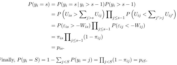
for s = 1,2, . . . , S. Note that πiS = 1 and biS = 1−PS−1j=1 bij by construction. Defining yi = s if and only if bis = 1 and bij = 0 for all j 6= s, then one has a strick-breaking representation for the multinomial probability parameter as

P(yi =s| {πis}_1,S) =P(bis= 1)Q

j6=sP(bij = 0) =πis

Q

j<s(1−πij), (3)

which, as expected, recovers pis by substituting the definitions of πis shown in (2).

The finite stick-breaking construction in (3) can be further generalized to an infinite setting, as widely used in Bayesian nonparametrics (Hjort et al., 2010). For example, the stick-break construction of Sethuraman (1994) represents the length of the kth stick using the product ofkstick-specific probabilities that are independent, and identically distributed (i.i.d.) beta random variables. It represents a size-biased random permutation of a Dirichlet process (DP) (Ferguson, 1973) random draw, which includes countably infinite atoms whose weights sum to one. The stick-breaking construction of Sethuraman (1994) has also been generalized to represent a draw from a random probability measure that is more general than the DP (Pitman, 1996; Ishwaran and James, 2001; Wang et al., 2011a).

Related to this paper, one may further consider making the stick-specfic probabilities depend on the covariates (Dunson and Park, 2008; Chung and Dunson, 2009; Ren et al., 2011). For example, the logistic stick-breaking process of Ren et al. (2011) uses the product ofk covariate-dependent logistic functions to parameterize the probability of thekth stick. To implement a stick-breaking process mixture model, truncated stick-breaking represen-tations with a finite number of sticks are commonly used, with inference developed via both Gibbs sampling (Ishwaran and James, 2001; Dunson and Park, 2008; Rodriguez and Dunson, 2011) and variational approximation (Blei and Jordan, 2006; Kurihara et al., 2007; Ren et al., 2011).

2.3 Logistic Stick Breaking

The stick-breaking construction parameterizes each pis with the product of s probability

parameters and links each yi with a unit-norm binary vector (bi1, . . . , biS), where biyi = 1

and bij = 0 a.s. if j 6=yi. Following the logistic stick-breaking construction of Ren et al.

(2011), one may represent pis with (3) and parameterize the logit of each πis with a latent Gaussian variable wis as πis = ewis_/PS

j=1ewij. To model observed or latent multinomial

variables, a stick-breaking procedure, closely related to that of Ren et al. (2011), is used in Khan et al. (2012) to transform the modeling of multinomial probability parameters into the modeling of the logits of binomial probability parameters using Gaussian latent

variables. As shown in Linderman et al. (2015), this procedure allows using the P´

olya-Gamma data augmentation, without requiring the assistance of the technique of Holmes and Held (2006), to construct Gibbs sampling that simultaneously updates all categories in each MCMC iteration, leading to improved performance over the one proposed in Polson et al. (2013).

The simplification brought by the stick-breaking representation, which stochastically arranges its categories in decreasing order, comes with a clear change in that it removes the invariance of the multinomial distribution to label permutation. While the loss of invariance to label permutation may not pose a major issue for Bayesian mixture models inferred with MCMC (Jasra et al., 2005; Kurihara et al., 2007), it appears to be a major obstacle when applying stick breaking for multinomial regression, where the performance is often found

to be sensitive to how the labels of the S categories are ordered. In particular, if one

constructs a logistic stick breaking model by letting logit(πis) =wis =x0_iβ_s, which means

πis = (1 +e−x0iβs₎−1_{, then one has}

pis= 1 +e−x0iβs−1Q

j<s 1 +e x0

iβj−1_,

which clearly tends to impose fewer geometric constraints on the classification decision boundaries of a category with a smallers. For example,pi1= 1 +e−x0iβ1−1 _{is larger than}

50% ifx0_iβ₁>0 whilepi2= 1 +ex 0

iβ1−1 _{1 +e}−x0iβ2−1 _{is possible to be larger than 50%}

only if both x0_iβ₁ < 0 and x0_iβ₂ > 0. We will use an example to illustrate this type of geometric constraints in Section 6.1.

Under the logistic stick-breaking construction, not only could the performance be sen-sitive to how theS different categories are ordered, but the imposed geometric constraints could also be overly restrictive even if the categories are appropriately ordered. Below we address the first issue by introducing a permuted and augmented stick-breaking rep-resentation for a multinomial model, and the second issue by adding the ability to model nonlinearity.

3. Permuted and Augmented Stick Breaking

Bayesian multinomial one. The paSB construction infers a one-to-one mapping between the labels of the S categories and the indices of the S latent sticks, transforming the problem

from modeling a multinomial random variable into modeling S conditionally independent

binary ones. It not only allows for parallel computation within each MCMC iteration, but also improves the mixing of MCMC in comparison to the one used in Polson et al. (2013), which updates one regression-coefficient vector conditioning on all the others, as will be shown in Section 6.5. Note that the number of distinct one-to-one label-stick mappings

is S!, which quickly becomes too large to exhaustively search for the best mapping as S

increases. Our experiments will show that the proposed MCMC algorithm can quickly es-cape from a purposely poorly initialized mapping and subsequently switch between many different mappings that all lead to similar performance, suggesting an effective search space that is considerably smaller than S!.

3.1 Category-Stick Mapping and Data Augmentation

The proposed paSB construction randomly maps a category to one and only one of the S

latent sticks and makes the augmented Bernoulli random variables {bis}1,S conditionally

independent to each other given {πis}1,S. Denote z = (z1, . . . , zS) as a permutation of

(1, . . . , S), wherezs∈ {1, . . . , S}is the index of the stick that categorysis mapped to. Given the label-stick mappingz, let us denotepis(z) as the multinomial probability of categorys,

and πizs(xi,βs) as the covariate-dependent stick probability that is associated with the

covariates of observation i and the stick that category s is mapped to. For notational

convenience, we will write πizs(xi,βs) as πizs and πij(xi,βs:zs=j) as πij. We emphasize

that here thesth regression-coefficient vectorβ_s is always associated with both categorys

and the corresponding stick probabily πizs, a construction that will facilitate the inference

of the label-stick mapping z. The following Theorem shows how to generate a categorical

random variable ofS categories with a set ofS conditionally independent Bernoulli random variables. This is key to transforming the problem from solving multinomial regression into solvingS binary regressions independently.

Theorem 1 Suppose yi ∼PSs=1pis(z)δs, where [pi1(z), . . . , piS(z)] is a multinomial

prob-ability vector whose elements are constructed as

pis(z) = (πizs)

1(zs6=S) Y j<zs

(1−πij), (4)

then yi can be equivalently generated under the permuted and augmented stick-breaking

(paSB) construction as

yi ∼ S

X

s=1

n

[1(bizs = 1)]

1(zs6=S)Q

j<zs1(bij = 0)

o

δs, (5)

bij ∼Bernoulli(πij), j∈ {1, . . . , S}. (6)

Distinct from the conventional stick breaking in (2) that maps category s to stick s

and makes bis depend on bij, j = 1, . . . , s−1, under the new construction in (5)-(6), the

the augmented binary random variables {bij}j become mutually independent given{πij}j.

Given yi, we still have bij = 0 for j < zyi and biz_yi = 1 a.s., but impose no restriction

on any bij for j > zyi, whose conditional posteriors given yi and πij remain the same as

their priors. These changes are key to appropriately ordering the latent sticks, more flexibly parameterizing πizs and hencepis(z), and maintaining tractable inference.

With paSB, the problem of inferring the functional relationship between the categorical

response yi and the corresponding covariates xi is now transformed into the problem of

modelingS conditionally independent binary regressions as

bizs|xi,βs∼Bernoulli[πizs(xi,βs)], i= 1, . . . , N, s= 1, . . . , S.

Note that the only requirement for the binary regression model under paSB is that it uses the Bernoulli likelihood. In other words, it uses the cross entropy loss (Murphy, 2012) as

− N

X

i=1

lnP(bizs|xi,βs) = N

X

i=1

−bizslnπizs(xi,βs)−(1−bizs) ln[1−πizs(xi,βs)] .

A basic choice is paSB logistic regression that lets

πizs(xi,βs) = 1/(1 +e −xiβs_),

which becomes the same as the logistic stick breaking construction described in Section 2.3 if zs = s for all s ∈ {1, . . . , S}. Another choice is paSB-robit regression that extends robit regression of Liu (2004), a robust binary classifier using cross entropy loss, into a robust Bayesian multinomial classifier. In robit regression, observation i is labeled as 1 if

x0_iβ+εi >0 and as 0 otherwise, whereεiare independently drawn from at-distribution with

κ degrees of freedom, denoted as εi iid∼ tκ. Consequently, the conditional class probability function of robit regression is P(yi = 1|xi,β) = Fκ(x0iβ), where Fκ is the cumulative

density function of tκ. The robustness is attributed to the heavy-tail property of Fκ(x0_iβ), which, if κ < 7, imposes less penalty than the conditional class probability function of logistic regression does on misclassified observations that are far from the decision boundary.

Applying Theorem 1, the category probability of paSB-robit regression with κ degrees of

freedom is shown in (4), whereπizs(xi,βs) =Fκ(x0iβs). The paSB-robit regression provides

a simple solution to robust multiclass classification; with {bij}i,j defined in Theorem 1, we

run independent binary robit regressions using the Gibbs sampler proposed in Liu (2004). In addition to paSB, we define permuted and augmented reverse stick breaking (parSB) in the following Corollary.

Corollary 2 Suppose yi∼PSs=1pisδs and pis(z) = (1−πizs)

1(zs6=S)Q

j<zsπij,

then yi can also be generated under the permuted and augmented reverse stick-breaking

(parSB) representation as

yi ∼ S

X

s=1

n

[1(bizs = 0)]

1(zs6=S)Q

j<zs1(bij = 1)

o

δs, (7)

Generally speaking, if πizs(xi,−βs) = 1−πizs(xi,βs), which is the case for logistic stick

breaking and robit stick breaking, whereπizs are defined as (1 +e

−x0_iβs₎−1 _{and Fκ(x}0 iβs),

respectively, and Bayesian multinomial SVMs to be discussed in Section 5, then there is no need to introduce parSB as an addition to paSB. Otherwise, there are potential benefits, such as for softplus regressions to be introduced in Section 4, to combine parSB with paSB.

3.2 Inference of Stick Variables and Category-Stick Mapping

Below we first describe Gibbs sampling for the augmented stick variables{bij}1,S, and then

introduce a Metropolis-Hastings (MH) step to infer the category-stick mapping z. Given

the category label yi, stick probabilityπij, and z, we samplebij as

(bij|yi, πij,z)∼1(j =zyi) +1(j > zyi)Bernoulli(πij),

forj= 1, . . . , S−1, and let

biS =1(zyi =S).

This means we let bij = 0 if j < zyi, bij = 1 if j = zyi, draw bij from Bernoulli(πij)

if zyi < j < S, and let biS = 1 if and only if zyi = S. Note that stick S is used as a

reference stick and πiS is not used in defining pis(z) in (4). Despite having no impact

on computing {pis}1,S, we inferπiS (i.e., sample the regression-coefficient vector βs0_:z s0=S)

under the likelihood QN

i=1Bernoulli(biS;πiS) and use it in a Metropolis-Hastings step, as

described in (8) shown below, to decide whether to switch the mappings of two different

categories, if one of which is mapped to the reference stick S. Once we have an MCMC

sample of{bij}1,S, we then essentially solve independentlyS binary classification problems,

thejth of which can be expressed asbij|xi,βs:zs=j ∼Bernoulli[πij(xi,βs:zs=j)].

Analogously, for parSB, {bij}1,S can be sampled as (bij|yi, πij,z)∼1(j < zyi) +1(j > zyi)Bernoulli(πij) forj = 1, . . . , S−1, andbiS = 1−1(zyi =S),which means we letbij = 1

ifj < zyi, let bij = 0 ifj =zyi, drawbij from Bernoulli(πij) if zyi < j < S, and let biS = 0

if and only if zyi =S.

Since stick-breaking multinomial classification is not invariant to the permutation of its class labels, it may perform substantially worse than it could be if the inherent geometric constraints implied by the current ordering of the labels make it difficult to adapt the decision boundaries to the data. Our solution to this problem is to infer the one-to-one mapping between the category labels and stick indices from the data. We construct a Metropolis-Hastings (MH) step within each Gibbs sampling iteration, with a proposal of switching two sticks that categories c and c0, 1≤c < c0 ≤S, are mapped to, by changing the current category-stick one-to-one mapping from z= (z1, . . . , zc, . . . , zc0, . . . , z_S) to z0=

(z₁0, . . . , z_S0) := (z1, . . . , zc0, . . . , zc, . . . , zS). Assuming a uniform prior on z and proposing

(c, c0) uniformly at random from one of the S₂

=S(S−1)/2 possibilities, we would accept the proposal with probability

min (

Y

i

QS

s=1[pis(z0)]1(yi=s)

QS

s=1[pis(z)]1(yi=s)

, 1 )

= min   

 

Y

i

QS

s=1

h (πiz0

s)

1(z0_s6=S)Q

j<z0

s(1−πij) i1(yi=s)

QS

s=1

h (πizs)

1(zs6=S)Q

j<zs(1−πij)

i1(yi=s), 1   

 

.

3.3 Sequential Decision Making

Random utility models, including both the logit and probit models as special examples, are widely used to infer the functional relationship between a categorical response variable and its covariates. For discrete choice analysis in econometrics (Hanemann, 1984; Greene,

2003; Train, 2009), these models assume that among a set of S alternatives, an individual

makes the choice that maximizes his/her utilityUis =Vis+εis, whereVis andεis represent

the observable and unobservable parts ofUis, respectively. If Vis is set asVis =x0iβs, then

marginalizing out εi = (εi1, . . . , εiS)0 leads to MLR if all εis follow the extreme value

dis-tribution (McFadden, 1973; Greene, 2003; Train, 2009), and multinomial probit regression if all εi follow a multivariate normal distribution (Albert and Chib, 1993; McCulloch and

Rossi, 1994; McCulloch et al., 2000; Imai and van Dyk, 2005).

Instead of examining the utilities of all choices before making the decision, the paSB construction is characterized by a sequential decision making process, described as follows. In step one, an individual decides whether to select the choice mapped to stick 1, or to select a choice among the remaining alternatives, i.e., choices {s:zs ∈ {2, . . . , S}}. If the

individual selects the choice mapped to stick 1, then the sequential process is terminated. Otherwise this choice is eliminated and the individual proceeds to step two, in which he/she would follow the same procedure to either select the choice mapped to stick 2 or proceed to the next step to select a choice among the remaining alternatives, i.e., choices {s:zs∈ {3, . . . , S}}. The individual, reconsidering none of the eliminated choices, will keep making a one-vs-remaining decision at each step until the termination of the sequential decision making process.

This unique sequential decision making procedure relaxes the independence of irrelevant alternatives (IIA) assumption, as described in the following Lemma.

Lemma 3 Under the paSB construction, the probability ratio of two choices are influenced by the success probabilities of the sticks that lie between these two choices’ corresponding sticks. In other words, the probability ratio of two choices will be influenced by some other choices if they are not mapped to adjacent sticks.

As in Lemma 3, the paSB construction could adjust how two choices’ probability ratio depends on the other alternatives by controlling the distance between the two sticks that they are mapped to, and hence provide a unique way to relax the IIA assumption. While the widely used MLR can be considered as a random-utility-maximization model with the IIA assumption, the paSB multinomial logistic model performs sequential random utility maximization that relaxes this assumption, as described in Lemma 5 in the Appendix.

4. Bayesian Multinomial Softplus Regression

Softplus regression uses the interaction of multiple hyperplanes to construct a union of convex-polytope-like confined spaces to enclose the data labeled as “1,” which are hence separated from the data labeled as “0”. It is constructed under a Bernoulli-Poisson link (Zhou, 2015) that thresholds at one a latent Poisson count, with the distribution of the Poisson rate defined as the convolution of the probability density functions of K experts,

each of which corresponds to the stack ofT gamma distributions with covariate-dependent

scale parameters. The number of expertsK and the number of layersT can be considered

as the two model parameters that determine the nonlinear capacity of the model. More specifically, for expert k, denotingrk as its weight andβt+1k as its tth regression-coefficient

vector, the conditional class probability can be expressed as

P(yi= 1|xi,{rk,{β(t+1)_k }1,T}1,K) = 1− K

Y

k=1

(1−pik),

pik= 1−1+ex0iβ

(T+1)

k _ln

n

1+ex0iβ

(T)

k _ln

h

1+. . .ln

1+ex0iβ

(2)

k

io−rk

;

when K=T = 1, the conditional class probability reduces to

P(yi = 1|xi, r,β) = 1−

1 1 +ex0iβ

r ;

and when K =T =r= 1, it becomes the same as that of binary logistic regression. Note

that a gamma process, a random draw from which is expressed asG =P∞

k=1rkδ{βt_k+1}1,T,

can be used to support a potentially countably infinite number of experts for softplus regression. For this reason, one can set K as large as permitted by computation and relies on the gamma process’s inherent shrinkage mechanism to turn off unneeded model capacity (not allK experts will be used ifK is set to be sufficiently large).

4.1 paSB and parSB Extensions of Softplus Regressions

We first follow Zhou (2016) to define

ς(x1, . . . , xt) = ln (1 +ext_{ln{1 +e}xt−1_{ln [1 +. . .ln (1 +e}x1_)]})

as the stack-softplus function. Note that if t = 1, the stack-softplus function reduces to softplus function ς(x) = ln(1 +ex), which is often considered as a smoothed version of the rectifier function, expressed as rectifier(x) = max(0, x), that has become the dominant nonlinear activation function for deep neural networks (Nair and Hinton, 2010; Glorot et al.,

2011; Krizhevsky et al., 2012; LeCun et al., 2015). We then parameterize λizs = −ln(1−

πizs), the negative logarithms of the failure probabilities of the stick that category s is

mapped to, as

λizs = ∞

X

k=1

rskς x0β(2)_sk, . . . ,x0β(T_sk+1), (9)

where the countably infinite atoms (β(2)_sk, . . . ,β(T_sk+1)) and their weights{rsk}k constitute a

continuous base distribution over a complete separable metric space Ω and 1/cs as a scale

parameter. In other words, we letbizs ∼Bernoulli(πizs) or

bizs ∼Bernoulli

"

1−

∞

Y

k=1

1+ex0iβ

(T+1)

sk _ln

n

1+ex0iβ

(T)

sk _ln

h

1+. . .ln

1+ex0iβ

(2)

sk

io−rsk

#

.

(10)

As shown in Theorem 10 of Zhou (2016), bizs can be equivalently generated from a

hierarchical model that convolves countably infinite stacked gamma distributions, with covariate-dependent scales, as

θ(T_isk)∼Gammarsk, ex 0 iβ

(T+1)

sk

,

. . .

θ(t)_isk∼Gammaθ(t+1)_isk , ex0iβ

(t+1)

sk

,

. . .

θ(1)_isk∼Gamma

θ(2)_isk, ex0iβ

(2)

sk

,

bizs =1(mis ≥1), mis= ∞

X

k=1

m(1)_isk, m(1)_isk ∼Pois(θ(1)_isk), (11)

the marginalization of whose latent variables lead to (10). Note the gamma distribution

θ∼Gamma(r,1/c) is defined such that E[θ] =r/c and var[θ] =r/c2, and the hierarchical structure in (11) can also be related to the augmentable gamma belief network proposed in Zhou et al. (2016). We consider the combination of (11) and either paSB in (5) or parSB in (7) as the Bayesian nonparametric hierarchical model for multinomial softplus regression (MSR) that is defined below.

Definition 1 (Multinomial Softplus Regression) With a draw from a gamma process for each category that consists of countably infinite atoms β(2:T_sk +1) with weights rsk > 0,

where β(t)_sk ∈ RP+1, given the covariate vector xi and category-stick mapping z, MSR

pa-rameterizes pis, the multinomial probability of category s, under the paSB construction as

pis(z) =

1−Q∞

k=1

1+ex0iβ

(T+1)

sk ln

n

1+ex0iβ

(T)

sk ln

h

1+. . .ln1+ex0iβ

(2)

sk

io−rsk 1(zs6=S)

×Q

j:zj<zs

"

Q∞

k=1

1+ex0iβ

(T+1)

jk _ln

1+ex0iβ

(T)

jk _ln

1+. . .ln

1+ex0iβ

(2)

jk

−rjk # ,

and parameterizes pis under the parSB construction as

pis(z) =

Q∞

k=1

1+ex0iβ

(T+1)

sk ln

n

1+ex0iβ

(T)

sk ln

h

1+. . .ln

1+ex0iβ

(2)

sk

io−rsk 1(zs6=S)

×Q

j:zj<zs

"

1−Q∞

k=1

1+ex0iβ

(T+1)

jk _ln

1+ex0iβ

(T)

jk _ln

1+. . .ln

1+ex0iβ

(2)

jk

For the convenience of implementation, we truncate the number of atoms of the gamma process atKby choosing a discrete base measure for each category asGs0=PK

k=1 γs0

Kδβ(2:_skT+1),

under which we have rsk ∼Gamma(γs0/K,1/cs0) as the prior distribution for the weight

of expert kin categorys. For each category, we expect only some of itsK experts to have non-negligible weights ifK is set large enough, and we may useP

k1

P

im (1) isk >0

, where

m(1)_isk is defined in (11), to measure the number of active experts inferred from the data.

4.2 Geometric Constraints for MSR

Since by definition we havepis(z) =πizs 1−

P

j<spis(z)

=πizs

Q

j<zs(1−πij) in MSR, it

is clear that ifπij for allj < zs are small andπizs is the first one to have a large probability

value close to one,yiwill be likely assigned to categorysregardless of how large the values of

{πij}j>zs are. To motivate the use of the seemingly over-parameterized sum-stack-softplus

function in (9), we first consider the simplest case ofK=T = 1. Without loss of generality, let us assume that the category-stick mapping is fixed atz = (1, . . . , S).

Lemma 4 For paSB-MSR with K = T = 1 and z = (1, . . . , S), the set of solutions to

pis(z)> p0 in the covariate space are bounded by a convex polytope defined by the intersec-tion of s linear hyperplanes.

Note that the binary softplus regression with K = T = 1 is closely related to logistic

regression, and reduces to logistic regression ifr = 1 (Zhou, 2016). With Lemma 4, it is clear

that even if an optimal category-stick mapping z is provided, paSB-MSR with K=T = 1

may still clearly underperform MLR. This is because category s uses a single hyperplane

to separate itself from the remaining S−scategories, and hence uses the interaction of at

most s hyperplanes to separate itself from the other S−1 categories. By contrast, MLR

uses a convex polytope bounded by at mostS−1 hyperplanes for each of theS categories.

WhenK >1 and/orT >1, an exact theoretical analysis is beyond the scope of this pa-per. Instead we provide some qualitative analysis by borrowing related geometric-constraint analysis for softplus regressions in Zhou (2016). Note that Equation (10) indicates that a noisy-or model (Pearl, 2014; Srinivas, 1993), commonly appearing in causal inference, is used at each step of the sequential one-vs-remaining decision process; at each step, the binary outcome of an observation is attributed to the disjunctive interaction of many possible hid-den causes. Roughly speaking, to enclose categorysto separate it from the remainingS−s

categories in the covariate space, paSB-MSR with K >1 and T = 1 uses the complement

of a convex-polytope-bounded space, paSB-MSR with K = 1 and T > 1 uses a

convex-polytope-like confined space, and paSB-MSR with both K > 1 and T > 1 uses a union

of convex-polytope-like confined spaces. For parSB-MSR with K+T > 1, the

5. Bayesian Multinomial Support Vector Machine

Support vector machines (SVMs) are max-margin binary classifiers that typically minimize a regularized hinge loss objective function as

l(β, ν) =

N

X

i=1

max(1−bix0_iβ,0) +νR(β),

wherebi ∈ {−1,1}represents the binary label for theith observation,R(β) is a

regulariza-tion funcregulariza-tion that is often set as the L1 orL2 norm of β,ν is a tuning parameter, and x0i

is the ith row of the design matrix X= (x1, . . . ,xn)0. For linear SVMs,xi is the covariate

vector of the ith observation, whereas for nonlinear SVMs, one typically set the (i, j)th element ofXas the kernel distance between the covariate vector of theith observation and the jth support vector. The decision boundary of a binary SVM is {x:x0β = 0} and an observation is assigned the labelyi= sign(x0β), which meansbi= 1 ifx0β≥0 andbi =−1

ifx0β<0.

5.1 Bayesian Binary SVMs

It is shown in Polson and Scott (2011) that the exponential of the negative of the hinge loss can be expressed as a location-scale mixture of normals as

L(bi|xi,β) = exp

−2 max(1−bix0iβ,0)

= Z ∞

0

1

√

2πωi exp

−1

2

(1 +ωi−bix0_iβ)2

ωi

dωi.

Consequently, L(b|X,β) = Q

iL(bi|xi,β) = exp{−2

P

imax(1−bix 0

iβ,0)} can be

re-garded as a pseudo likelihood in the sense that it is unnormalized with respect to b =

(b1, . . . , bN)0 ∈ {−1,1}N. This location-scale normal mixture representation of the hinge

loss allows developing close-form Gibbs sampling update equations for the regression coeffi-cientsβvia data augmentation, as discussed in detail in Polson and Scott (2011) and further generalized in Henao et al. (2014) to construct nonlinear SVMs amenable to Bayesian in-ference. While data augmentation has made it feasible to develop Bayesian inference for SVMs, it has not addressed a common issue that SVMs provide the predictions of determin-istic class labels but not class probabilities. For this reason, below we discuss how to allow SVMs to predict class probabilities while maintaining tractable Bayesian inference via data augmentation.

Following Sollich (2002) and Mallick et al. (2005), by defining the joint distribution of β and {xi}i to be proportional to Qi[L(1|xi,β) +L(−1|xi,β)], one may define the

conditional distribution of the binary label bi∈ {−1,1} as

P(bi|xi,β) =



 

 

1

1 +e−2bix0_iβ, for|x

0

iβ| ≤1;

1

1 +e−bi[x0_iβ+sign(x0_iβ)], for|x 0

iβ|>1;

(12)

the penalty termνR(β) of the regularized hinge loss can be related to a corresponding prior

distribution imposed on β, such as Gaussian, Laplace, and spike-and-slab priors (Polson

and Scott, 2011).

5.2 paSB Multinomial Support Vector Machine

Generalizing previous work in constructing Bayesian binary SVMs, we propose multinomial SVM (MSVM) under the paSB framework that is distinct from previously proposed MSVMs (Crammer and Singer, 2002; Lee et al., 2004; Liu and Yuan, 2011). A Bayesian MSVM that predicts class probabilities has also been proposed before in Zhang and Jordan (2006), which, however, does not have a data augmentation scheme to sample the regression coefficients in closed form, and consequently, relies on a random-walk Metropolis-Hastings procedure that may be difficult to tune.

Redefining the label sample space from bi ∈ {−1,1} tobi∈ {0,1}, we may rewrite (12)

asbi|xi,β∼Bernoulli[πi,svm(xi,β)], where

πi,svm(xi,β) =



 

 

1

1 +e−2xiβ, for|x

0

iβ| ≤1;

1

1 +e−xiβ−sign(x0_iβ), for|x 0

iβ|>1.

(13)

The Bernoulli likelihood based cross-entropy-loss binary classifier, whose covariate-dependent probabilities are parameterized as in (13), is exactly what we need to extend the binary SVM into a multinomial classifier under paSB introduced in Theorem 1. More specifically, given the category-stick mapping z, with the success probabilities of the stick that cate-gory s is mapped to parameterized asπizs,svm(xi,βs) and binary stick variables drawn as bizs ∼Bernoulli[πizs,svm(xi,βs)], we have the following definition.

Definition 2 (paSB multinomial SVM) Under the paSB construction, given the co-variate vectorxiand category-stick mappingz, multinomial support vector machine (MSVM)

parameterizes pis, the multinomial probability of category s, as

pis(z) = [πizs,svm(xi,βs)]1(zs 6=S)Y

j:zj<zs

πizj,svm(xi,βj).

Note that there is no need to introduce parSB-MSVM in addition to paSB-MSVM, since by definition, we have πizs,svm(xi,−βs) = 1−πizs,svm(xi,βs) for all s.

6. Example Results

Constructed under the paSB framework, a multinomial regression model of S categories is

characterized by not only how the S stick-specific binary classifiers with cross entropy loss parameterize their covariate-dependent probability parameters, but also how itsScategories

are one-to-one mapped to S latent sticks. To investigate the unique properties of a paSB

multinomial regression model, we will study the benefits of both inferring an appropriate

mappingzand increasing the modeling capacity of the underlying binary regression model.

6.1 Influence of Binary Regression Model Capacity

We first consider the Iris data set with S = 3 categories. We choose the sepal and petal

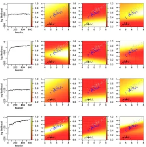
lengths as the two dimensional covariates to illustrate the performance of MSR under four different settings. We fix z = (1,2,3), which means category s is mapped to stick s for all s, but choose different model capacities by varying K andT.

Examining the relative 2D spatial locations of the observations, where the blue, black, and gray points are labeled as category 1, 2, and 3, respectively, one can imagine that setting z= (2,1,3), which means mappings categories 2, 1, and 3 to the 1st, 2nd, and 3rd sticks, respectively, will already lead to excellent class separations for MSR withK=T = 1, according to the analysis in Section 4.2 and also confirmed by our experimental results (not shown for brevity). More specifically, with the 2nd, 1st, and 3rd categories mapped to the 1st, 2nd, and 3rd sticks, respectively, one can first use a single hyperplane to separate category 2 (black points) from both categories 1 (blue points) and 3 (gray points), and then use another hyperplane to separate category 1 (blue points) from category 3 (gray points). However, when the mapping is fixed atz= (1,2,3), as shown in the first row of Figure 1,

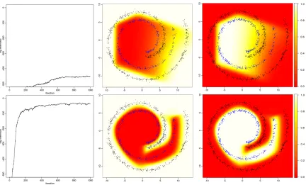
MSR with K = T = 1 performs poorly and fails to separate out category 1 (blue points)

right in the beginning. This is not surprising since MSR withK =T = 1 is only equipped

with a single hyperplane to separate the category that the first stick is mapped to (category

z1 = 1 in this case) from the others, whereas for this data set it is apparent at least two

hyperplanes are required to separate the blue from the black and gray points. MSR with

K = 5 andT = 1 also fails to work withz = (1,2,3), as shown in the third row of Figure 1, which is also not surprising since it can only use the complementary of a convex-polytope-bound confined space to enclose categoryz1 = 1, but the blue points can not be enclosed in such a manner. Despite purposely enforcing an unfavorable category-stick mapping, once

we increase T, the performance quickly improves, which is expected since T > 1 allows

using a single (if K= 1 as in the second row) or a union (ifK >1 as in the fourth row) of convex-polytope-like confined spaces to separate one category from the others (by enclosing the positively labeled observations in each stick-specific binary classification task).

The results in Figure 1 show that even an unoptimized category-stick mapping, which

is unfavorable to MSR with smallK and/orT, is enforced, empowering each stick-specific

binary regression model with a higher capacity (using larger K and/or T) can still allow

MSR to achieve excellent separations. It is also simple to show that for the data set in Figure 1, even if one chooses low-capacity stick-specific binary regression models by setting

T = 1, one can still achieve good performance with MSR if the category-stick mapping is

set asz= (2,1,3),z= (3,1,2),z= (2,3,1), orz= (3,2,1). That is to say, as long as it is

not category 1 (blue points) that is mapped to stick 1, MSR withT = 1 is able to provide

satisfactory performance.

6.2 Influence of Category-Stick Mapping and its Inference

The Iris data set in Figure 1 provides an instructive example to show not only the importance of increasing the model capacity if a poor category-stick mapping is imposed, but also the importance of optimizing the category-stick mapping if the capacities of these stick-specific

binary regression models are limited. To further illustrate the benefits of inferring an

Figure 1: Log-likelihood plots and predictive probability heat maps for the 2-D iris data with a fixed category-stick mapping z= (1,2,3). Blue, black, and gray points are labeled

as categories 1, 2, and 3, respectively. For the first row, K = 1 and T = 1, second row,

K = 1 andT = 3, third row, K = 5 andT = 1, and fourth row, K = 5 and T = 3. The

log-likelihood plots are shown in Column 1, and the predictive probability heat maps of categories 1 (blue), 2 (black), and 3 (gray) are shown in Columns 2, 3, and 4, respectively.

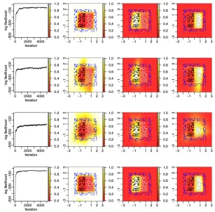
We show that for MSR, even if bothKandT are sufficiently large to allow each stick-specific binary regression model to have a high enough capacity, whether an optimal category-stick mapping is selected may still clearly matter for the performance.

As shown in the first three rows of Figure 2, with K =T = 10, three differentz’s are considered andz= (1,2,3) (shown in the first row) is found to perform the best. As shown

in the fourth row, we samplez using (8) within each MCMC iteration and achieve a result

that seems as good as fixingz= (1,2,3). In fact, we find that our inferred mappings switch betweenz = (1,2,3) andz= (1,3,2) during MCMC iterations, indicating that the Markov

chain is mixing well. These results suggest the importance of both learning the mappingz

from the data and allowing the stick-specific binary classifiers to have enough capacities to model nonlinear classification decision boundaries.

When sampling z = (z1, . . . , zS) that the S categories are mapped to, although S!

Figure 2: Log-likelihood plots and predictive probability heat maps for the square data

with K = T = 10. The blue, black, and gray points are labeled as categories 1, 2, and 3,

respectively. We fix the category-stick mapping asz= (1,2,3) for Row 1, (2,1,3) for Row 2, and (3,1,2) for Row 3, and sample z for Row 4. The log-likelihood plots are shown in Column 1, and the predictive probability heat maps of categories 1 (blue), 2 (black), and 3 (gray) are shown in Columns 2, 3, and 4, respectively.

the proposed MH step, proposing two indices zj and zj0 to switch in each iteration, is a

simple but effective strategy to escape from the mappings that lead to poor fits. Note that the probability of azj not being proposed to switch aftertMCMC iterations is [(S−2)/S]t.

Even if S is as large as 100, this probability is less than 10−8 at t= 1000. Also note the iteration at whichzj is proposed to switch at the first time follows a geometric distribution, with success probability 2/S. ThusS/2 is the expected number of iterations for a zj to be

proposed to switch once.

To demonstrate the efficiency of our permutation scheme, we construct square101, a syn-thetic two-dimensional data set consisting of 101 categories. We generate 8000 data points that are uniformly at random distributed within the 12×12 spatial region occupied by all 101 categories. The decision boundaries of different classes are displayed in Figure 3(a), where the data points placed within the outside square frame, whose outer and inner di-mensions are 12 and 10, respectively, are assigned to category 1, and these placed within the

Although it is almost impossible to search for the best category-stick mappingzgiving rise to the highest likelihood from all 101!≈10160 possible mappings, we show our permutation scheme is very effective in escaping from poor mappings, leading to a performance that is comparable to the best of those obtained with pre-fixed suboptimal mappings. More specifically, applying the analysis in Section 4.2 to Figure 3(a), we expect an aSB-MSR

to perform well under a fixed suboptimal category-stick mapping z, where z1 = 1, which

means the outside square frame is mapped to stick 1, and the squares closer to the inner boundary of the square frame are mapped to the sticks broken at earlier stages; the mapping

z = (1,2,· · · ,101) is such an example. In other words, we first separate the frame from all the other squares, and then sequentially separate the squares from the remainders; the closer a square is from the frame, the earlier it is separated. The total number of suboptimal mappings z’s constructed in this manner is as large as 36!×28!×20!×12!×4!≈1099.5.

First, we uniformly at random generate 3600 different suboptimal mappings z’s under

this construction, run aSB-MSR with K = T = 4, and plot the histogram of the 3600

log-likelihoods in Figure 3(b). Second, we start from 3600 randomly initialized z, run

paSB-MSR with K = T = 4, and also plot the histogram of the 3600 log-likelihoods in

Figure 3(b). For each run, we choose 20,000 MCMC iterations and collect the last 1000 MCMC samples. Each log-likelihood is averaged over those of the corresponding model’s collected MCMC samples. As in Figure 3(b), the log-likelihood from a paSB-MSR is in general clearly larger than that of an aSB-MSR with a fixed suboptimalz, and there is little

overlap between their corresponding histograms. Further examining the 3600 z’s inferred

by paSB at its last MCMC iteration shows that 3482 of them have z1 = 1 and all of them

have z1 ≤5. Supposez1 ∈ {/ 1,2,3,4,5} at the current iteration, which means category 1 is mapped to none of the first five sticks, then the probability of not only selecting stickz1, but

also switching it with one of the first five sticks in the MH proposal is ₁₀₁1 ×₁₀₀5 . Thus the probability that category 1 has never been proposed to mapped to one of the first five sticks after t iterations is [1−5/(101×100)]t, which becomes as small as 0.005% att= 20,000, demonstrating the effectiveness of our permutation scheme in dealing with a large number of categories. Note we have also tried 3600 aSB-MSR, each of which is provided with a

randomly initialized z. The log-likelihoods, however, are all far below −4000 and hence

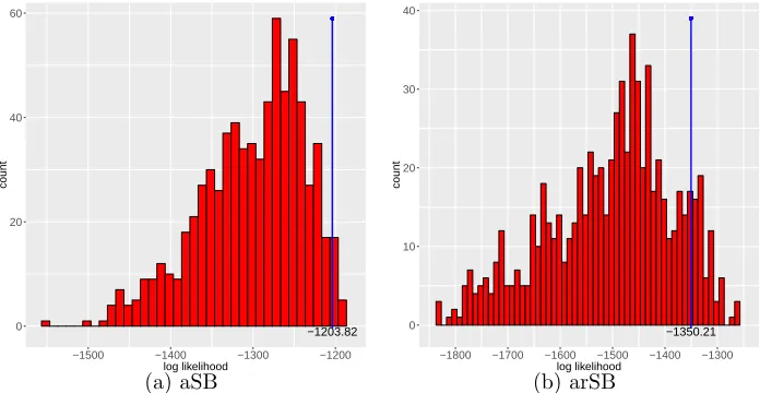
not included for comparison. This phenomenon is not surprising, as the probability for a randomly initializedzto be suboptimal is as tiny as 36!×28!×20!×12!×4!/101!≈10−60.5. Figure 4 empirically demonstrates the effectiveness of permutingzon the satimage data set, using MSRs withK = 5,T = 3, andz fixed at each of the 6! = 720 possible one-to-one category-stick mappings. Panels (a) and (b) show the log-likelihood histograms for MSRs constructed under augmented SB (aSB) and augmented reversed SB (arSB), respectively. Both histograms are clearly left skewed, indicating under both aSB and arSB, only a small proportion of the 720 different category-stick mappings lead to very poor fits. The blue vertical lines at −1203.82 in (a) and−1350.21 in (b) are the log-likelihoods by paSB and

parSB, respectively, in both of which the category-stick mapping z is updated by a MH

step in each MCMC iteration. Only 20 (97) out of 720 aSB-MSRs (arSB-MSRs) have a higher likelihood than paSB-MSR (parSB-MSR).

1 1 1 1 2 3 4 5 6 7 8 9 10 11 37 38 39 40 41 42 43 44 45 12 36 65 66 67 68 69 70 71 46 13 35 64 85 86 87 88 89 72 47 14 34 63 84 97 98 99 90 73 48 15 33 62 83 96 101 100 91 74 49 16 32 61 82 95 94 93 92 75 50 17 31 60 81 80 79 78 77 76 51 18 30 59 58 57 56 55 54 53 52 19 29 28 27 26 25 24 23 22 21 20 (a) 0 100 200 300 400

−4200 −4000 −3800 −3600 −3400 log likelihood

count

aSB paSB

(b)

Figure 3: (a) Illustration of the square101 data and (b) log-likelihood histograms, by aSB-MSR with 3600 random suboptimal category-stick mappings and by paSB-aSB-MSR with 3600 randomly initialized category-stick mappings.

−1203.82 ● ● ● ● ● ● ● ● ● ● ● ● ● ● ● ● ● ● ● ● ● ● ● ● ● ● ● ● ● ● ● ● ● ● ● ● ● ● ● ● ● ● ● ● ● ● ● ● ● ● ● ● ● ● ● ● ● ● ● ● ● ● ● ● ● ● ● ● ● ● ● ● ● ● ● ● ● ● ● ● ● ● ● ● ● ● ● ● ● ● ● ● ● ● ● ● ● ● ● ● ● ● ● ● ● ● ● ● ● ● ● ● ● ● ● ● ● ● ● ● ● ● ● ● ● ● ● ● ● ● ● ● ● ● ● ● ● ● ● ● ● ● ● ● ● ● ● ● ● ● ● ● ● ● ● ● ● ● ● ● ● ● ● ● ● ● ● ● ● ● ● ● ● ● ● ● ● ● ● ● ● ● ● ● ● ● ● ● ● ● ● ● ● ● ● ● ● ● ● ● ● ● ● ● ● ● ● ● ● ● ● ● ● ● ● ● ● ● ● ● ● ● ● ● ● ● ● ● ● ● ● ● ● ● ● ● ● ● ● ● ● ● ● ● ● ● ● ● ● ● ● ● ● ● ● ● ● ● ● ● ● ● ● ● ● ● ● ● ● ● ● ● ● ● ● ● ● ● ● ● ● ● ● ● ● ● ● ● ● ● ● ● ● ● ● ● ● ● ● ● ● ● ● ● ● ● ● ● ● ● ● ● ● ● ● ● ● ● ● ● ● ● ● ● ● ● ● ● ● ● ● ● ● ● ● ● ● ● ● ● ● ● ● ● ● ● ● ● ● ● ● ● ● ● ● ● ● ● ● ● ● ● ● ● ● ● ● ● ● ● ● ● ● ● ● ● ● ● ● ● ● ● ● ● ● ● ● ● ● ● ● ● ● ● ● ● ● ● ● ● ● ● ● ● ● ● ● ● ● ● ● ● ● ● ● ● ● ● ● ● ● ● ● ● ● ● ● ● ● ● ● ● ● ● ● ● ● ● ● ● ● ● ● ● ● ● ● ● ● ● ● ● ● ● ● ● ● ● ● ● ● ● ● ● ● ● ● ● ● ● ● ● ● ● ● ● ● ● ● ● ● ● ● ● ● ● ● ● ● ● ● ● ● ● ● ● ● ● ● ● ● ● ● ● ● ● ● ● ● ● ● ● ● ● ● ● ● ● ● ● ● ● ● ● ● ● ● ● ● ● ● ● ● ● ● ● ● ● ● ● ● ● ● ● ● ● ● ● ● ● ● ● ● ● ● ● ● ● ● ● ● ● ● ● ● ● ● ● ● ● ● ● ● ● ● ● ● ● ● ● ● ● ● ● ● ● ● ● ● ● ● ● ● ● ● ● ● ● ● ● ● ● ● ● ● ● ● ● ● ● ● ● ● ● ● ● ● ● ● ● ● ● ● ● ● ● ● ● ● ● ● ● ● ● ● ● ● ● ● ● ● ● ● ● ● ● ● ● ● ● ● ● ● ● ● ● ● ● ● ● ● ● ● ● ● ● ● ● ● ● ● ● ● ● ● ● ● ● ● ● ● ● ● ● ● ● ● ● ● ● ● ● ● ● ● ● ● ● ● ● ● ● ● ● ● ● ● ● ● ● ● ● ● ● ● ● ● ● ● ● 0 20 40 60

−1500 −1400 −1300 −1200 log likelihood count (a) aSB −1350.21 ● ● ● ● ● ● ● ● ● ● ● ● ● ● ● ● ● ● ● ● ● ● ● ● ● ● ● ● ● ● ● ● ● ● ● ● ● ● ● ● ● ● ● ● ● ● ● ● ● ● ● ● ● ● ● ● ● ● ● ● ● ● ● ● ● ● ● ● ● ● ● ● ● ● ● ● ● ● ● ● ● ● ● ● ● ● ● ● ● ● ● ● ● ● ● ● ● ● ● ● ● ● ● ● ● ● ● ● ● ● ● ● ● ● ● ● ● ● ● ● ● ● ● ● ● ● ● ● ● ● ● ● ● ● ● ● ● ● ● ● ● ● ● ● ● ● ● ● ● ● ● ● ● ● ● ● ● ● ● ● ● ● ● ● ● ● ● ● ● ● ● ● ● ● ● ● ● ● ● ● ● ● ● ● ● ● ● ● ● ● ● ● ● ● ● ● ● ● ● ● ● ● ● ● ● ● ● ● ● ● ● ● ● ● ● ● ● ● ● ● ● ● ● ● ● ● ● ● ● ● ● ● ● ● ● ● ● ● ● ● ● ● ● ● ● ● ● ● ● ● ● ● ● ● ● ● ● ● ● ● ● ● ● ● ● ● ● ● ● ● ● ● ● ● ● ● ● ● ● ● ● ● ● ● ● ● ● ● ● ● ● ● ● ● ● ● ● ● ● ● ● ● ● ● ● ● ● ● ● ● ● ● ● ● ● ● ● ● ● ● ● ● ● ● ● ● ● ● ● ● ● ● ● ● ● ● ● ● ● ● ● ● ● ● ● ● ● ● ● ● ● ● ● ● ● ● ● ● ● ● ● ● ● ● ● ● ● ● ● ● ● ● ● ● ● ● ● ● ● ● ● ● ● ● ● ● ● ● ● ● ● ● ● ● ● ● ● ● ● ● ● ● ● ● ● ● ● ● ● ● ● ● ● ● ● ● ● ● ● ● ● ● ● ● ● ● ● ● ● ● ● ● ● ● ● ● ● ● ● ● ● ● ● ● ● ● ● ● ● ● ● ● ● ● ● ● ● ● ● ● ● ● ● ● ● ● ● ● ● ● ● ● ● ● ● ● ● ● ● ● ● ● ● ● ● ● ● ● ● ● ● ● ● ● ● ● ● ● ● ● ● ● ● ● ● ● ● ● ● ● ● ● ● ● ● ● ● ● ● ● ● ● ● ● ● ● ● ● ● ● ● ● ● ● ● ● ● ● ● ● ● ● ● ● ● ● ● ● ● ● ● ● ● ● ● ● ● ● ● ● ● ● ● ● ● ● ● ● ● ● ● ● ● ● ● ● ● ● ● ● ● ● ● ● ● ● ● ● ● ● ● ● ● ● ● ● ● ● ● ● ● ● ● ● ● ● ● ● ● ● ● ● ● ● ● ● ● ● ● ● ● ● ● ● ● ● ● ● ● ● ● ● ● ● ● ● ● ● ● ● ● ● ● ● ● ● ● ● ● ● ● ● ● ● ● ● ● ● ● ● ● ● ● ● ● ● ● ● ● ● ● ● ● ● ● ● ● ● ● ● ● ● ● ● ● ● ● ● ● ● ● ● ● ● ● ● ● ● ● ● ● ● ● ● ● ● ● ● ● ● ● ● ● ● ● ● ● ● ● ● 0 10 20 30 40

−1800 −1700 −1600 −1500 −1400 −1300 log likelihood

count

(b) arSB

Figure 4: Log-likelihood histograms for MSRs using all 720 possible category-stick map-pings, constructed under (a) augmented stick breaking (aSB) and (b) augmented and re-versed stick breaking (arSB). The blue lines in (a) and (b) correspond to the log-likelihoods of paSB-MSR and parSB-MSR, respectively.

modeling capacity of the binary classifier. However, even with a low-capacity binary classi-fier, the performance could be significantly improved if that difficult-to-separate category is mapped to a larger-indexed stick, for which there are fewer categories left to be separated in its “one-vs-remaining” binary classification problem. Examining thez’s associated with the 100 lowest log-likelihoods in Figure 4, we find there are 51 mappings belonging to the set {z :z5 = 1 or z6 = 1} in aSB, and 77 belonging to {z :z3 = 1 or z6 = 1} in arSB. It

suggests that separating Categories 5 or 6 (Categories 3 or 6) from all the other categories

0

50

100

150

200

250

Expert k rk

● ●

● ●

●

● ● ● ● ●

1 2 3 4 5 6 7 8 9 10

● category 1 category 2 category 3

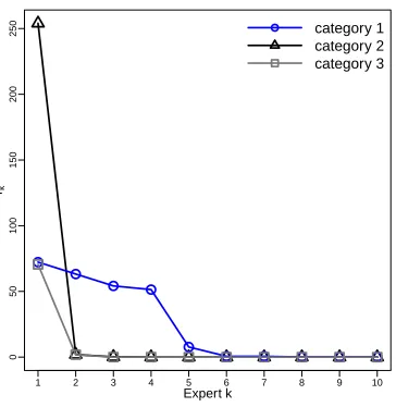
Figure 5: Inferred expert weights rk in descending order for each category of the square

data with K=T = 10.

the aSB (arSB) construction. But if breaking the sticks associated with these categories at late stages, we only need to separate them from fewer remaining categories, which could be much easier. We have further examined the other 620 arrangements, and found no evident

patterns. These observations suggest that the effective search space of the mapping z is

considerably smaller thanS!, and the proposed MH step is effective in escaping from poor category-stick mappings.

In paSB-MSVM, we use a Gaussian radial basis function kernel, whose kernel width is cross validated from a set of predefined candidates. We find its performance to be sensitive to the setting of the kernel width, which is a common issue for SVMs (Cherkassky and Ma, 2004; Soares et al., 2004; Chang et al., 2005). If an appropriate kernel width could

be identified through cross validation, we find that learning the mapping z becomes less

important for paSB-MSVM to perform well. However, we find that if the kernel width is not well selected, which can happen if all candidate kernel widths are far from the optimal value, the binary classifier for each category may not have enough capacity for nonlinear classification and the learning of the category-stick mappingzcould then become important.

6.3 Turning Off Unneeded Model Capacities

While one can adjust both K and T to control the capacity of binary softplus regression,

for MSR, the total number of experts K is a truncation level that can be set as large as

permitted by the computation budget. This is because the truncated gamma process used by each stick-specific binary softplus regression shrinks the weights of unnecessary experts

towards zeros. Figure 5 shows in decreasing order the inferred weights of the experts

belonging to each of the 3 categories of the square data set. These weights are inferred by

MSR with K =T = 10 and the learning of z, as in the fourth row of Figure 2. It is clear

Figure 6: First row: classification of a 2-D swiss roll data by paSB-MSR withK = 5,T = 3,

using the original covariates. Second row: paSB-MSR with K = 5, T = 1 trained on the

covariates transformed via the paSB-MSR used in the first row. In each row, the left column plot the log-likelihood against MCMC iteration, and the middle and right columns show the predictive probability heatmaps for Category 1 (black points) and Category 2 (blue points), respectively.

of the corresponding classification decision boundaries shown in the fourth row of Figure 2. We note that while T is a parameter to be set by the user, we find increasing it increases model capacity, without observing clear signs of overfitting for all the data considered here.

6.4 MSR with Data Transformation

then augment the original covariate vector xi as

˜

xi:=

x0_i,log 1 +ex0iβ˜

(2)

11_{,· · · ,log 1 +e}x0iβ˜

(t+1)

jk _{,· · · ,log 1 +e}x0iβ˜

(T+1)

SK

0

(14)

and run another MSR with the transformed covariates ˜xi.

For illustration, we show the efficacy of this data-transformation strategy on a 2-D swiss

roll data in Figure 6. The first row shows the results of MSR withK = 5 andT = 3, using

the original covariates xi, while the second row shows MSR withK = 5 and T = 1, using

the transformed covariates ˜xidefined by (14), where the regression coefficient vectors ˜β (t+1) jk

are learned using the MSR illustrated in the first row. It is evident that the classification is greatly improved in terms of both training log-likelihood and out-of-sample predictions.

6.5 Results on Benchmark Data Sets

To further evaluate the performance of the proposed paSB multinomial regression mod-els, we consider paSB multinomial logistic regression (paSB-MLR), paSB multinomial robit

with κ = 6 degrees of freedom (paSB-robit), paSB multinomial support vector machine

(paSB-MSVM), and MSRs. We compare their performance with those of L2 regularized

multinomial logistic regression (L2-MLR), support vector machine (SVM), and adaptive

multi-hyperplane machine (AMM), and consider the following benchmark multi-class clas-sification data sets: iris, wine, glass, vehicle, waveform, segment, dna, and satimage. We also include the synthetic square data shown in Figure 2 for comparison. For SVM we use the LIBSVM package, which trainsS(S−1)/2 one-vs-one binary classifiers and makes

prediction using majority voting (Chang and Lin, 2011). We run LIBSVM in Rwith

pack-agee1071 (Meyer et al., 2015). We consider MSRs with (K, T) as (1,1), (1,3), (5,1), and

(5,3), respectively. We also consider MSR with data transformation (DT-MSR), in which

we first train a MSR with K = 5 and T = 3 to transform the covariates and then stack

another MSR with K = 5 and T = 1. We provide detailed descriptions on the data and

experimental settings in the Appendix.

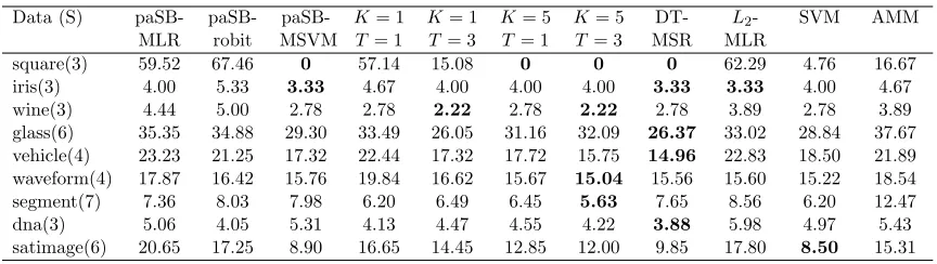
With the number of categories in parentheses right after the data set names, we sum-marize in Table 1 the classification error rates by various models, where those of MSRs are

calculated by averaging over paSB and parSB. Table 1 shows that an MSR with K or T

sufficiently large generally outperforms paSB-MLR, paSB-robit, L2-MLR, and AMM, and

using another MSR on the transformed covariates can in general further reduce the error rate. This is especially evident when there are nonlinearly separable categories, as indicated

by a clearly higher error rate of L2-MLR in contrast to that of SVM. One may notice that

paSB-robit, paSB-MLR, and MSR with K = T = 1 are similar to L2-MLR in terms of

performance, suggesting the effectiveness of the proposed permutation scheme, which helps mitigate the potential adverse effects of having asymmetric class labels. One may also note that paSB-robit outperforms paSB-MLR on glass, vehicle, waveform, dna, and satimage, indicating there are benefits in using a robust classifier on these data sets. Comparable error rates of paSB-MSVM to SVM and better performance of MSRs on most data sets demonstrate the success of the paSB framework in transforming a binary classifier with cross entropy loss into a Bayesian multinomial one.

Data (S) paSB-MLR

paSB-robit

paSB-MSVM

K= 1 T = 1

K= 1 T = 3

K= 5 T= 1

K= 5 T = 3

DT-MSR

L2

-MLR

SVM AMM

square(3) 59.52 67.46 0 57.14 15.08 0 0 0 62.29 4.76 16.67 iris(3) 4.00 5.33 3.33 4.67 4.00 4.00 4.00 3.33 3.33 4.00 4.67 wine(3) 4.44 5.00 2.78 2.78 2.22 2.78 2.22 2.78 3.89 2.78 3.89 glass(6) 35.35 34.88 29.30 33.49 26.05 31.16 32.09 26.37 33.02 28.84 37.67 vehicle(4) 23.23 21.25 17.32 22.44 17.32 17.72 15.75 14.96 22.83 18.50 21.89 waveform(4) 17.87 16.42 15.76 19.84 16.62 15.67 15.04 15.56 15.60 15.22 18.54 segment(7) 7.36 8.03 7.98 6.20 6.49 6.45 5.63 7.65 8.56 6.20 12.47 dna(3) 5.06 4.05 5.31 4.13 4.47 4.55 4.22 3.88 5.98 4.97 5.43 satimage(6) 20.65 17.25 8.90 16.65 14.45 12.85 12.00 9.85 17.80 8.50 15.31

Table 1: Comparison of the classification error rates (%) of MLR, robit,

paSB-MSVM, MSRs with various K and T (columns 5 to 8), MSR with data transformation

(DT-MSR), L2-MLR, SVM, and AMM.

among the collected ones for all paSB models, and summarize in Table 4 of the Appendix the classification error rates of various models, with the number of inferred support vectors or active hyperplanes included in parenthesis. Following the definition of active experts in

Zhou (2016), we define for MSRs the number of active hyperplanes asTPS

s Kse whereKse is the number of active experts for class s. The number of active hyperplanes determines the computational complexity for out-of-sample prediction with a single MCMC sample, which is O(TPS

s Kse ). Since the error rates of MSRs in Table 4 are calculated by averaging over

both paSB and parSB, the number of active hyperplanes isTPS

s(Ke

(paSB) s +Ke

(parSB) s ).

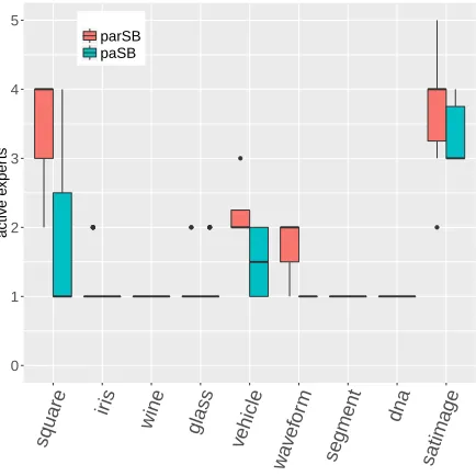
Shown in Figure 8 in the Appendix are boxplots of the number of each category’s active

experts for MSR with K = 5 and T = 3. Except for several categories of satimage that

require all K = 5 experts for parSB-MSR, K = 5 is large enough to provide the needed

model capacity under all the other scenarios. As shown in Table 4, MSRs with sufficiently

largeKand/orT are comparable to both SVM and paSB-MSVM in terms of the error rates,

while clearly outperforming them in terms of the number of (active) hyperplanes/support vectors and hence computational complexity for out-of-sample predictions. While MSR

withK =T = 1, paSB-MLR, and paSB-robit generally perform worse than SVM in terms

of the error rates, they use much fewer hyperplanes and hence have significantly lower computation for out-of-sample predictions. In summary, MSR whose upper-bound for the

number of active expects K and number of layers for each expert T can both be adjusted

to control its capacity of modeling nonlinearity, can achieve a good compromise between the accuracy and computational complexity for out-of-sample prediction of multinomial class probabilities, and can be further improved by training an additional MSR on the transformed covariates.

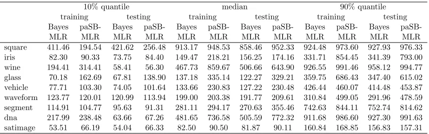
We further measure how well the Gibbs sampler is mixing using effective sample size (ESS) for both paSB-MLR and Bayesian multinomial logistic regression (Bayes MLR) of Polson et al. (2013). For both algorithms we let β_j ∼ N0,diag(α_j0−1, . . . , α−1_jV)

, where

αjv ∼ Gamma(0.001,1/0.001). The ESS (Holmes and Held, 2006) of a parameter or a

function of parameters is defined as ESS =L/[1 + 2P∞

h=1ρ(h)],whereLis the number of

10% quantile median 90% quantile training testing training testing training testing Bayes

MLR

paSB-MLR Bayes

MLR

paSB-MLR Bayes

MLR

paSB-MLR Bayes MLR

paSB-MLR

Bayes MLR

paSB-MLR

Bayes MLR

paSB-MLR square 411.46 194.54 421.62 256.48 913.17 948.53 858.46 952.33 924.48 973.60 927.93 976.33 iris 82.30 90.33 73.75 84.40 149.47 218.21 156.25 174.16 331.71 854.45 341.39 793.00 wine 194.41 314.41 58.41 56.30 467.73 859.67 506.66 643.90 926.55 991.46 958.12 994.77 glass 70.18 162.69 67.81 138.90 137.18 335.14 122.27 329.21 359.75 686.43 347.40 615.02 vehicle 77.71 103.30 74.05 101.64 133.66 230.83 127.22 230.48 426.44 460.07 414.48 453.87 waveform 123.77 120.01 120.99 113.94 199.00 203.38 191.77 209.61 310.84 499.05 291.96 478.59 segment 114.91 104.77 95.63 91.31 281.11 294.17 270.63 355.46 742.63 844.11 752.74 814.62 dna 217.99 238.48 63.66 67.26 481.65 736.58 505.59 772.32 911.68 986.60 927.30 991.63 satimage 53.51 66.19 54.04 66.33 82.50 90.50 81.87 90.11 160.84 168.85 156.83 157.31

Table 2: Comparison of the ESS of the conditional class probability between Bayes MLR and paSB-MLR.

Since the Gibbs sampler of Bayes MLR samples one β_j conditioning on allβ_j0 for j0 6=j,

which may lead to strong dependencies between different categories and hence slow down the mixing of the Markov chain. By contrast, theβ_j’s are conditionally independent given

the augmented variables bij’s in paSB-MLR, which may lead to faster mixing. For both

Bayes MLR and paSB-MLR, we consider five independent random trials, in each of which we randomly initialize the model parameters, run 10,000 Gibbs sampling iterations, and

collect the last 1,000 MCMC samples of β_j. We use the mcmcse package (Flegal et al.,

2016) to estimate the ESS of each pij in a random trial using the 1,000 collected MCMC

samples. For the training set, we calculate the 10% quantile, median, and 90% quantile of the ESSs of all pij for each random trial, and then report their averages over the five

random trials in Table 2. For the testing set, we follow the same steps and report the results in Table 2. While paSB-MLR underperforms Bayes MLR on some of the data sets for the 10% ESS quantile, they consistently outperform Bayes MLR on all data sets for both the ESS median and 90% ESS quantile, for both training and testing.

6.6 Robustness of paSB-Robit Regression

We use the contaminated vehicle data to demonstrate the robustness of paSB-robit. As discussed by Liu (2004), the heavy-tailed conditional class probability function of robit regression can robustify the decision boundary when there exist outliers. We use the vehicle training set as inliers, synthesize outliers that are far from inliers, combine both as the new training set, and keep the testing set unchanged. We generate different numbers of outliers so that the ratio of outliers to inliers varies from 0, 0.1, 0.2, 0.3, to 0.5, at each of which we randomly simulate 10 different sets of outlier covariates. We provide the details on how we generate outliers in the Appendix.

We compareL2-MLR and paSB-robit withκ= 1 degree of freedom on the contaminated

vehicle data. Figure 7 shows the prediction error rate (mean ±standard deviation) of the

testing set for different outlier-inlier ratios. When there are no outliers, both approaches

delivers comparable performances. As the ratio increases, paSB-robit withκ= 1 more and