Consistency, Breakdown Robustness, and Algorithms for Robust Improper Maximum Likelihood Clustering

Consistency, Breakdown Robustness, and Algorithms for

Robust Improper Maximum Likelihood Clustering

Pietro Coretto [email protected]

Department of Economics and Statistics University of Salerno

Fisciano (SA), Italy

Christian Hennig [email protected]

Department of Statistical Science University College London London, United Kingdom

Editor:Ingo Steinwart

Abstract

The robust improper maximum likelihood estimator (RIMLE) is a new method for robust multivariate clustering finding approximately Gaussian clusters. It maximizes a pseudo-likelihood defined by adding a component with improper constant density for accommo-dating outliers to a Gaussian mixture. A special case of the RIMLE is MLE for multi-variate finite Gaussian mixture models. In this paper we treat existence, consistency, and breakdown theory for the RIMLE comprehensively. RIMLE’s existence is proved under non-smooth covariance matrix constraints. It is shown that these can be implemented via a computationally feasible Expectation-Conditional Maximization algorithm.

Keywords: Robustness, Improper density, Mixture models, Model-based clustering,

Maximum likelihood, ECM-algorithm

1. Introduction

Maximum likelihood estimation (MLE) in a Gaussian mixture model with mixture com-ponents interpreted as clusters is a popular approach to cluster analysis (see, e.g., Fraley and Raftery (2002)). In many datasets not all observations can be assigned appropriately to clusters that can be properly modelled by a Gaussian distribution, and it is also well known that the MLE can be strongly affected by outliers (Hennig (2004)). In this paper we investigate the recently introduced “robust improper maximum likelihood estimator” (RIMLE, see Coretto and Hennig, 2016), a method for robust clustering with clusters that can be approximated by multivariate Gaussian distributions. The basic idea of RIMLE is to fit an improper density to the data that is made up by a Gaussian mixture density and a “pseudo mixture component” defined by a small constant density, which is meant to capture outliers and observations in low density areas of the data that cannot properly be assigned to a Gaussian mixture component (called “noise” in the following). This is inspired by the addition of a uniform “noise component” to a Gaussian mixture suggested by Banfield and Raftery (1993). Hennig (2004) showed that using an improper density improves the breakdown robustness of this approach for one-dimensional datasets. As in

c

many other statistical problems, violations of the model assumptions may cause problems in cluster analysis. Our general attitude to the use of statistical models in cluster analysis is that the models should not be understood as reflecting some underlying but in practice unobservable “truth”, but rather as thought constructs implying a certain behaviour of methods derived from them (e.g., maximizing the likelihood), which may or may not be appropriate in a given application (more details on the general philosophy of clustering can be found in Hennig and Liao (2013); Hennig (2015b)). Using a model such as a mixture of multivariate Gaussian distributions, interpreting every mixture component as a “cluster”, implies that we look for clusters that are approximately “Gaussian-shaped”, but we do not want to rely on whether the data really were generated i.i.d. by a Gaussian mixture. We

focus on situations in which the number of clustersGis fixed.

There is a number of proposals already in the literature for accounting for the presence of noise and outliers in model-based clustering problems. The contributions can be divided in two groups: methods based on mixture modelling, and methods based on fixed partition models. Within the first group Banfield and Raftery (1993) and Coretto and Hennig (2011) dealt with uniform distributions added as “noise components” to a finite Gaussian

mix-ture. Peel and McLachlan (2000) proposed to model data based on Studentt-distributions.

Cuesta-Albertos et al. (1997) and Garc´ıa-Escudero and Gordaliza (1999) introduced and

studied trimming in order to robustify thek-means partitioning method. Robust

partition-ing methods with homoscedastic clusters based on ML–type procedures where proposed in Gallegos (2002) and Gallegos and Ritter (2005). Heteroscedasticity in ML-type partition-ing methods has been introduced with the TCLUST algorithm of Garc´ıa-Escudero et al. (2008) and the “k–parameters clustering” of Gallegos and Ritter (2013). More references and an in-depth overview are given in Garc´ıa-Escudero et al. (2015). Different from the methods based on fixed partition models, mixture models and RIMLE allow a smooth transition between different clusters and between clustered observations and noise, which improves parameter estimation in the presence of overlap between mixture components. The one-dimensional version of the RIMLE was introduced in Coretto and Hennig (2010) and was investigated based on Monte Carlo experiments. Extension of the methods to the multivariate setting is not straightforward. Existence and consistency of the MLE for the multivariate Gaussian mixtures is a long standing problem due to the ill-posedness of the likelihood function. Even for ML for plain multivariate Gaussian mixtures (i.e. the RIMLE with the improper constant density set to zero), consistency theory is limited to the situa-tion in which the model is assumed to hold precisely, and restrictive condisitua-tions are required (e.g., Redner and Walker (1984)). Chen and Tan (2009) and Alexandrovich (2014) propose and study a penalized ML estimator. Garc´ıa-Escudero et al. (2014) studied a classification ML estimator for Gaussian mixture that is based on the TCLUST idea.

3.2. The consistency results given here in Section 4 are of a nonparametric nature and show the consistency of the RIMLE for the RIMLE-functional defined for a general class of sampling distributions. Similar results have been shown for a partition likelihood model (Gallegos and Ritter (2013)) and for alternative, trimming-based approaches to robust clus-tering (e.g., Garc´ıa-Escudero et al. (2008); Gallegos and Ritter (2009)). Compared to these results, there is an additional difficulty for the RIMLE, namely that degeneration of the likelihood needs to be prevented also in the case that almost all observations are assigned to the noise component and the remaining observations are fitted arbitrarily well. This may look like a disadvantage, but in the literature cited above such problems are only avoided by fixing the trimming rate. An analysis like the one given here, and in Coretto and Hen-nig (2016), is required for understanding the case in which both the proportion of points considered as “noise” and the density level at which this happens are flexible. Coretto and Hennig (2016) introduce the OTRIMLE, a data-adaptive choice of the improper constant density, the method’s tuning constant for achieving robustness. That paper also includes a comprehensive simulation study comparing the different approaches to robust clustering. In the study, every method turns out to be superior for one or more setups, but the OTRIMLE achieves the most satisfactory overall performance.

The paper is organized as follows. We first discuss in Section 2 an artificial dataset to illustrate the issues RIMLE is meant to deal with. The RIMLE is introduced and defined in Section 3. In Section 4 existence and consistency of the RIMLE are proved. Section 5 treats the computation of the RIMLE and the choice of input parameters for the algorithms. Section 6 studies the breakdown robustness of RIMLE. Numerical experiments are presented in Section 7. Section 8 concludes the paper.

2. Artificial data examples

Every clustering method is designed to recover certain types of clusters even when they are based on methods and algorithms that apply universally. For instance, the well known

k-means method aims to discover spherical balanced clusters, although the algorithm will

find a solution when this is not the case. In this section we introduce some issues in robust clustering by showing examples of data affected by noise that cause trouble to most cluster-ing methods, includcluster-ing those that supposedly explicitly account for it. These examples will illustrate the kind of clustering problem that the method investigated in this paper aims

to address. Two artificial data sets are generated in dimension p= 20 from two sampling

designs, called AsyNoise and GEM respectively, also considered for the numerical experi-ments presented in Section 7. The two data sets are shown in Figure 1 and 3. A detailed description of the sampling designs is given in Section 7.

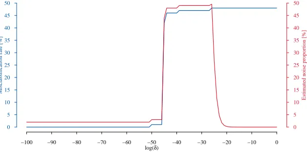
In AsyNoise (Figure 1) there are 500 observations in 5 moderately separated clusters from student-t distributions with varying degrees of freedom, 187 observations (37.4%) are background noise. We have symmetric and elliptical clusters that are not well separated along all directions, and they are of different size. Although there is a deviation from Gaussianity in the tails of the clusters’ distribution, methods based on Gaussian shapes are candidates to reconstruct such groups. Plain Gaussian mixture clustering (without noise

component) fixing the number of clusters at G= 5 using the popularR package mclust of

X1

−2 2 4 6 8 12

+ + + + + + + + + + + + + + + + + + + + + + + + + + + + + + + + + + + + + + + + + + + + + ++ + + + + + + + + + + + + + + + ++ + + + + + + + + + + + + + + + + + ++ + + + + + + + + + + + + + + + + + + + + + + + + + + + + + + + + + + + + + + + ++ + + + ++ + + + + + + + + + ++ + + + + + + + + + + + + + + + + + + + + + + + + + + + + ++ + + + + + + + + + + + + + + + + + 1

1 111 11 111 111111 11 11 1111 1111111 1111111111 11111

222 222 2 22222 2222 222 2222 22 222 222222 22 222₂2 2 2 2222_{22 2}2₂ 2 _{22 2}

22 22₂₂ 22_{2 2} 2

222 22 2₂ 2 2 2

2 222 ₃₃33 3 3 33_{333 33}3333

33 333333

4 444 4444 4444 44 444 44 444444 4444 4444444444 4444444 44

5 5555555 555555555555555 5 ₅₅₅5₅₅ 5555

5 ₅ 5 5 55 5 5 555 5 55555555

5 5 5 5 5555₅55 5 5 5 5 5

5 555 555 55 5

5 5

5555 555 5555 55 5555 5555 5555555555 + + + + + + + + + + + + + + + + + + + + + ++ + + + + ₊ + + + + + + + + + + + + + + + + + + + + + + + + + + + + + + + + + + + + + + + + + + + + + + + + + + + + + + + + + + + + + + + + + + + + + + + + + + + + + + + + + + + + + + + + + + + + + ++ + + + + + + + + + + + + + + + + + + + + + + + + + + + + + + + + + + + + + + + + + + + + + + + + + + + + + + + + + + + + + + + + 1 1 1 11 1111111 1 11111 1111111111111111111111111111

2 22 2 22 22 22 2 222222222222222222222222222222

2 22 2 2222₂₂22 22 22 22222 22₂ 2

2 2 222222 22₃₃322₃₃₃33223333233333333₃ 3333

44 44 4 4 4 44 44 4 44 444444444 44444444444444 4444444444554

55555555 5555 55 5 555 5 555555555 5555 5 555 5 5 5 5 5 55 555555555 5 5 55555 5555555555555555 55 5 55555555555 55 5 55 5 555 5 5₅555555 5 5 55

−2 2 4 6 8

+ + + + + + + + + + + + + + + + + ++ + + + + + + + + ₊ + + + + + + + + + + + + + + + + + + + + + + + + + + + + + + + + + + + + + + + + + + + + + + + + + + + + + + + ++ + + + + + + + + + + + + + + + + + + + + + + + + ++ + + + + + ++ + + + +++ + + + + + + ++ + + + + + + + + + + + + + + + + + + + + + + + + + + + + + + + + + + + + ++ + + + + + + + + + + + + ++ + + +1 1 11 11 1

1 111 1111111111111 111 1 11 11 11 111 1 11 11111 1

2 222 22 222 2 22 2 2 ₂

2 2 2 2 2 2 222222 2222222 2 22 22 222 22222 222₂22222 222 2222₂2

2 2 2 2 2222₂ 2 2 22_{3 3}333 33333 33 32_{3 3 3}23 3333 33 323

4 4 4 444 44 4444444 444 4 4 4444 4 44444 44 444444 4455544444444

5 5 5 5555

5 5 5 555 55555555 555 5555555

5 55 5₅5 5 55 5 5 55 5

5 55 5 55

5 5 5₅555555 5 555 55 5555555

55 5

5 555555 555555555

5 5 5555_{55 55}5555555

−20 0 10 20 + + + + + + + + + + + + + + + + + + + + + + + + + + + + + + + + + + + + + + + + + + + + + + + + + + + + + + + + + + + + + + + + + + + + + + + + + + + + + + + + + ++ ++ + + + + + + + + + + + + + + + + + + + + + + + + + + + + + + + ++ + + + + + + + + + ++ + + + + + ++ + + + + + + + + + + + + + + + + + + + + + + + + + + + + + + + + + + + + + + + + + + + + + + + + + + + 1 1 1111 111111111 1111 111 1 11111 1₁11 111111 1

1 1 1 11 1 1 2 2 2 222 22 2 2 222₂ 2 2 2222222222 2 2222 2 22 2₂ 22 222 2222 2 222 2 2 2 2 ₂₂

2 2 22222₂ 2 2

2 2

222 2 22₂332 2223222 3 33_{3 3}3 3 333333₃₃3_{3 33}33 3

444 44444 4 4 4 444 4 4 444 4 44444444 44 44444444554444444444

55 55 55 55 55 555 5

55 555 555 5 5 5555 5555 5₅ 555₅ 555555 5 5

5 5 5555

5 5 5 5₅ 5 5 ₅ 5 5 5 5 55 555 55 5555 5 5 5 5 555 5 5 55 55 5 55555555555555555555₅5

−2 2 4 6 8 12 ++ +++ + + + + + + + + + + + + + + + + ++ + + + + ++ + + + +++ + + + + ++ + + + + ++ + + + + + + + + +₊ + ++₊+++ + + + + + + + + + ++ + + + + + + + + + ++ + + + + + ₊+ ++++++ +++++ + +++ + +++ + + + ++ ++ +++++ + + + + + + + + + + + + ++ + + + + + + + + ++ + + + + + ++ ++ + + + + + + + + + + + + + + + + + + + + ++ + ++_{+ +} + ++ 1 111 111 1 1 1 1 1 1 11 1 11 1 11 1 1 111 1 1 1₁11 1 1 1 11 11 11 11 1 1 1 2 2 2 22₂ 2₂₂₂₂₂ 2 2 2 2 2 2 2 2 2 2 2 2 222 2 2 2 2 22 2 2 22₂ 2 2 2 2 2 2 2 22 2 2 2 2 2 2 22 2 2 2 2 2 22 2 2 2 2 2 22 2 2 2 2 2₂₂₂ 2 2 2 2 33 3 3 33 3 3 3 3 3 3 3 333

3 33 3 3 3 333 4 4444₄4 4 44 4 44 4 4 44 4 4 4 444 44444444 4 444 44 4 4444444 4 4 4 5 5 5 55 5 5 5 5 5 5 5 5 5 5 5 5 5 5 5 5 5 5 5 55 5 5 5 5 55 5 55

5 55 55 5 55 5 55 55 5 5 5 5 5 5 5 5 5 5 5 5 5 5 5 55 55 5 5 5 5 5 5 5 5 5 5 55 5 5 5 5 5 5 5 5 5 5 55 5 55555 5 5 5 55 5 5 5₅₅₅5 5 5 5 5 X2 + + ++ + + + + + + + + + + + + + + + + + ++ + + + + + + + + + ++ + + + + + + + ++ + + + + + + + + + + + + + + + ++₊+++ ₊ +++ + + + ++ ++ + + + + + + + ++ +++ + ++++ + + + + +++ + _{++ +} ++ + + + + ++ ++ +++++++++++++++ + + + + + + ++ + + + + + + + + + + + + + + + + + + + + + + + + + + + + + + + + + + + + + + + ++ + +++₊+ + + ++ 1 1 1 11 1 1 1 1 1 1 1 1 1 1 1 11 1 11 1 1 1 1 11 1 1 11 1 1 1 1 11 1 1 11₁ 1 111

2 22 2 22 2₂ 222 2 2222 2 2 2 2 2 222222 2 2222₂ 2 2 2 222 2 22 2 2 2 2222 2 2 2 2 22 2 2 2 2 222 2 2 2 2 2 2 22 2 2₂₂ 22₂₂2 2 2 3 3 3 3 3 3 3 3 3 3 3 3 33333 3 3 33 33334

4 44 4 4 4 4 4 44 44 4 4 44 4₄ 44₄₄444 4 4 4 4 4 4 44 4 4 4 4 4 4 44 444444

5 5 5 55 5 5 55 5 5 5 5 5 5 5 5 55 5 555 5 5 5 5555 55 5 5 5 5 55 5 5 5 5 5 5 5 5 5 5 5 5 5 55 5 5 5 5 5 5 5 5 5 55555 5 5 55 5 5 5 5 5 5 55 5 5 5 5 5 5 5 5 5 5 5 5 55 5₅5₅ 5 5 5 555 555555 5 5 5 5 ++++ + + + + + + + ++ + + + + ++ + + +++ + + + + + + + +++++ + + + ++++ + ++ + + ++ + + + + + + + +++₊₊ ++ + + ++ + + + + + + + + + + + + + + ++ +++++ + + ++ ++ +++++ ++ + +++++ + + +++ +++++++ + +++ + + + + + + + + + + + ++ + + + + + + + + + +++ + + + + +++++ + + ++ + + + + + + + + ++ + + + + + +++ + + ++ + + + 1 1 11 1 1 1 1 1 1₁ 1111₁

1 1 1 1111 1 11 1 1 11 1 1 1 1 1 1 1 1111

1 1 111

2 222 22 2_{22 2 22} 2 222

2 22 2 2

2 22222 2222 22

2 2

22 22 2 2 2 2 2 2222 2 2 2 2 2 2 2 2 2222222

2 2 2 2 2 2 2 2 2₂₂ 2 2 2 2 2 2 2 3 3 3 3 3 3 3 3 3 3 3 3 33 3 3 3 3 3 3 3 3 3 3 34

4 4 4_{4 44}4 44 4 4 4 44 4 4 4 44 4444 4 444444 4 44 444

4 444 4 4 44 4 4 4 5 5 5 5 5 5 5 5 5 5 5 5 5 5 5 5 5 55

5 5 55

5 5 5

5 5₅5 5 5 5 5 5 5 55 55 5 55 5 5 5 5 5 5 5 5 555₅ 5 5 5 5 5 5 5 555 5 5 5 5 55 5 5 5 5 5 5 55 5 5 5 5 5 5 5 5 5 55 55 55 5 5 ₅ 5 5 5 5 5 5 5 555

5 5 5 5 5 5 + + + ++ + + + + + + + ++ + ++ + ++ + ++ + + + + + ++ + + +++ + + + + ++ ++ + ++ + +₊ + + + + + + + + + + ++ + ++ + + + + + + + + +++ + + + + + + + + +++++ + ++ + + + + +++ ++ ++ + + + + + + + + ++ ++ + +₊+₊++++++₊+₊+ ₊₊ + + +++ ++ + + + + + + +++ + + + + + + + ++ + + + + + + + + + + + + + + + + + ++ ++ + + + ++ ++ ++ + 1 111 11 1 1

1 1 11 111 1 1 1 1 111 1 1 1 1 1 1 1 1 1 1 1 1 1 1 1 1 1 1 1 1 1 1 1 1 2 2 2 2 2 2222 2 22 2 2 2 2 2 2222

2 2222 2 2222

2 2 2 2

2 2_{2 2} 2

2 2

2 2 222 2 2 2 2 2 2 2 2 2 2 2 222 2 2 2 2 2 2 222 2 2₂₂

2 22 2 2 2 2 3 33 3 3 3 3

3 3 3 3 3 3 333 3 3 3 3 3 3 33 3

44444444 4 4 4 4 4

44 4 44 4 4444444444 44

4 4 ₄ 44 4 4 4 4 444 4 4 4 4 4 55 5 55 5 5 55 5 5 5 5 5 5 555 5

5 55 5 5 5 5 5 5 5 5 55 5 5 5 5 55 5 5 5 55 5 5 5 5 5 5 5 5 5 5 5 5 5 5 5 5 5 5 5 5 5 5 5 5 5 5 5 5 5 5 55 5 5 5 5 5 5 5 5 5 5 5 5 5 5 5 5 555 555 5 5 5 5 5 5 5 5 55 55 5 55 5 + + + + + + + + + + + + + + + + + + + + + ++ + + + + + + + + + + + + + + + + + + + + + + + + + + + + + + + + + + + + + + + + + + + + + + + + + + + + + + + + + + + + + + + + + + + + + + + + + + + + + + + + + + + + + + + + + + + + + + + + + + +++ + ₊ + + + + ++ + + + + + + + + + + + + + + + + + + + + + + + + + + + + + + + + + + + + + + + + + + + + + + + + + + + + + + + 1 1111₁₁₁ 1111111111 111111111111111111111111111₁2 222222 22222222222 22222222222222222222222222222222222₂₂2222222

2 2 2 2 2222222 2 2222 2 2 233 3 3 33 333333 3 3333 333₃3333

4 444444 4444444444444444 444444444₄4444 444444444 44555 5555 555555555555₅5555₅

5 5 555 55 5 5555555 555555 55555555 55 55₅5

5 5 55555555555

5 55 5

55 55 555555555555555555 55555555555555 +

+ + ++ + + + + + + + + + + + + + + + + + + + + + + + + + + + + + + + + + + + + ++ + + + + + + + + + + + + + + + + + + + ++ + + + + + + + + + + + + + + + + + + + + + + + + + + + + + + + + + + + + + + + + + + + + + + ++ + + + + + + + + + + + + + + + + + + + + + + + + + + + + + + + + + + + + + + + + + + + + + + + + + + + + + + + + + + + + + + + + + + + + + + + + + + + 1 1 111 11 111111 111 11 11 111 1 11 1111111 111111111₁1₁1

222 2222222₂2 222 2 22 222 2222 222 222222 222 222222 2222222 22 2 222222 222

22 2 2 2 22222 22

2 2 2

2 222 33 33333333 333₃333334444 43_{4 4}4 4433344444 44 4444444434444434444444 4 44 4 44 444 44

5 555555555555555 55 5 5₅55 5 5 55555 5555 55 555 55555 5 55 55555 555555 ₅ 5

5 5 555 5 5 5 55 5 555555 555 5 5 55 5

5 5 5 5 55555555555 55 5 555 555 5 5

5 5 X3 +

+ + + + + + + + + + + + + + + + + + + + + + + + + + + + + + + + + + + + ++ + + + ++ ++ + + + + + + + + + + + + + + + + + + + + + + + + + + + + + + + + + + + + + + + + + + + + + + + + + + + + + + ++ + + + + + + + + + + + + +₊ + + + +₊ +++ ++ + + + + ++ + + + + + + + + + + + + + + + + + + + + + + + + + + + + + + + + + + + + + + + + + + + + + + + + + + + + + + + 1 1 11 11111 1111111111111111 111111111 11₁ 1 11211212222 2 2112 2222 1

22 222 22 222 222 2 22222 22 22222222222222 22222222 2

2 22 2 2

22 2222 2 22222 2 2 23 32333_{33 3}233 33 3 323 3333 323

3 3 3 344 4 444 44 4444444 444 4 4 4444 4 4444444 45 5454_{555 5}4₄₄₄₄5 5554444455₄55454

5555555₅5 5 5 555₅ 5 5 555 55 5 555₅55555 55555 5555 5₅55

5 555 55 55 55 5555 555555 5555

555 5 5 5555 5 555 5 5

5 5 55 5555555 55 −20 0 10 20 + + + ++ + + + + + + + + + + + +₊ + + + + + + + + + + + + + + + + + + + + + + + + + + ++ + + + + + + + + + + + + + + + + + + + + + + + + + + + + + + + + + + + + + + + + + + + + + + ++ ++ + ++ + + + + + + + + + + + + + + + + + + + + +₊ + + + + + + + + + + + + + ++ + + + + + + + + + + + + + + + + + + + + + + + + + + + + + + + + + + + + + + + + + + + + + + + + + ++ 1 1 11_{11 1}1111₁₁11 1111 111 1 11 11 1111111 1111 11111211 12 222 2 22 222222 22 2 22 2222222222 2 22222222222222222222 2 2 2222222 2222222222222₂

2 2 22 22 2 23 33 3 344434443 33333 3 33333343 333343

4 4 4 444 4 4 44 4 4444444444444₄₄4₄4 44 4 444 4555 55 555555544555544

55 555₅5₅ 5

5 555 55 555 5 5 55 55 5 55555 5 5555555 55555₅ 5 5 5 5 5 5555 55 555 55 5555 55555555 55 55555 555555555555555₅55

−2 2 4 6 8 ++ +++ + + + + ++ ++ + + ++ +++++ + + + ++ + + + + + + + + + + + + + + + + + + + + + + + + + + + + + + + + + + + + + + + + + + + + + + +₊ + + + + + + + + +++ + + + + + + + ++ + + + +++ +++ + + + + + + + + + + + + ++ + + + +++ + ++ + + + ++ + + + + + + + + + + + + + + +++ + ++ + ++ ++ + + + + + + + + + + + + + ++ + + + + + + + + + + + + + 1+1+

1 1 1 1 1 1 111 1 1 1 1 111 111111₁11111₁₁1₁ 1 1 1 11 11 1 1 1 1 1 2 2 2 222 2222 2 2 2 2 2 2 2 2 2 2 2 2 2 2 222 2 2 2 2222 2 222 222 2 2 2 2 22 2 2₂2

2 2 2₂ 2 2 2 2 2 22 2 2 2 2 22

2 22 2 2 2 222 2 2 2 23 3 3 3 3 3 3 3 3 33 3 3 3₃33 3 33 3 3 3 3 3 4 444444 44444444 4 4 4 4 4 4 4 4 4 44 444 4 44

444 44 444444444 44555

5 5 5 5 5 5 5 55₅ 555

5 5 5 55

5 55 5 5 5 55 5 5 5 5 5 5 5 55 55 55555 5555

5 5 5 5 5 5 55 5

5 5 5 5 555 5 5 5 55 55 5 5 5 5 5 55 5 5 5 5 5 5 555 5 5 5 5₅₅55 5 5 5 5 5 5 5

55555555₅₅ + +

+ ++ + + + ++ + +++++++ ++++ ++ + + + + + + + + + + ++ + + + + + ++ + + + + + +++ + + + + + +++ + + ++ + + ++ + + + + + +₊ + + + + + + + + + + + + + + + + + + + + + + + + ++++ ++ + + + + + + + + + + ++ + + + + + + +++++ + + + ++₊ + + + + + + + + ++ + + + + + + + + + +++ ++ + + + ++ + + + + + + + + + + + + + ++ + + + + + + + + + +1 1

1 1 1 1 1 1 1 1 1 1 1 1 1 1 11 1 1111

1 1 1 11 1₁₁ 11 11

1 1 1111 1 1 11 1 2 2 2 222

2 222 2 2 2₂ 2 22 22 2 222 2 2 2 2 2 2 2

2 22 2 2 22

2 2 22222222 2₂2 22 2 ₂ 2 2 2 2 2 2 22 2 2 2 2 2 2 2 2 2 2 22 2 2 2 2 22 2 3 3 3 3 3 3 3 33 3 3 3 33 3 3₃ 3 3 3 3 3 3 3 3

4 444 4444 44 4 4 4 4 4 4 4 4 4 4 4 4 4 4 444 44 4 4 4 4 4 44 44

44 4

4 4 444 4 4

5 5 5 5

5 5 5 5 5555 5 5 5 5 5 5 5 55 5 5 5 5 5 5 5 5 5 5 5 5 5 5 5 55 55 5 5 555 5 55 5 5 5 5 5 5 5 5 5 5 5555555 5 5 5 5 55 5

5 55 55 55 5 5 5 5 5 5 5 5 5 5555

5 5 55 5 5 5 55 5 5 5 5 55 5 5 5 5 5 5 + + ++ + + + + + + + + + ++ +++ + +++ + ₊ + + + + + + + + + + + + + ++ + + ++ + + + ++ + ++ + + + + + + + + + + + + + + + + + + + + ++ ₊+ + + + + + + + ++ + + + + + + + + + + ++ +++ + +++ + + + + + + + + + + ++ + + + ++ + ++ + + + ₊ + + + + + + ₊ + + + + + + + ++ + + ++++ + + + + + + + + + + +++ + + + + + + + + + + + + + + + +++ + + +

+ + 11 ++

1 1 1 1 11 1 1 1 1 1 1 1 11111111 1 1 1 1 1 1 1 1 1 111 1 1 1 1 111 1

111

2 2 2 2 2₂ 22 22 2 2 2₂ 2 2 2 2 2 2 2 22 2 2 2 2 2 22 2222 2 2 2222 22 22 2 2222 2 2₂ 2 2₂ 2 2 2 2 2 22 22₂ 222 22 2 222 222 2 2 2 23 3 3 3 3 3 3 3 33 3 3 333₃3 3 3 3 3 33 3 3 44 4 4 4 4 4 44 44 4 444

4 4 4 4 4 4 4 4 4 44 44 4 4 44 44 4 4 4 4444444445544

5555 5 5 5 5 5₅5

5 55 5 5 5 5 5 55 5 5 5 5 555 5 5 5 5 5 555 5 5 5 5 5 55 55₅5 5 5 5 5 5 5 5555 5 5 5555 5 5 5 5 555 5 5 5 5 5 555 5 5 5 5 5 5 55 5 5 5 55 5 5 5 5 5 5 5 5 5 5 5555 5 55 5 55 X4 + + + ++ + + + + +++ +++ +++ ++ + + + + ++ + + + + + + + + + + + + + + + + + + ++ + + + + + + + + + + + + + + + + + + + + + + + + + + +++ + + + + + + + + ++ + + ++ + + + +₊ ++++++++++ + + + ++ + + + + + + + ++ + + + + + + + + + + + + + + +₊ + + + + + + + ++ + + + + + +++ + + + ++ + + + + + + + + + + + + + + + ++ + + + + + + + + + + + ++ + 1 1 1 1 1 1 1 1 1 1 1 1 1 1 1 1111 1111 1 1 1 1₁1₁11_{1 1}

1 1 1 1 1 111 1

1 1 12

2 2 222 22 2 222

2 ₂ 2 2₂222

2 2 2 2 2 2 2 2 2 2 2 2 22 2 2 222 2

2 2

2222 222 2 2 ₂ 2 ₂ 2 2 2 2 2 2 2 2 2 2 2 2 22

22 2 222222₂₂₂ 2 3 3 3 3 3 3 3 3 3 33

3 3 333 3 3 3 3 3 3 3 3 3

44444444 4 4

4 4₄4 44 4 4 4 4 4 4 4 4 4 4 4444

4 4

444444 4 4 4

44 45445544

5 5 5 5 5 5 5 5₅ 5 5 5 5 5 5 555 5 5 5 5 5 5 5 5 5 5 5 5 5 5 5 55 55 5 55 5555 5 55

5 5 5 5 5 5 555 5 5 5 5 5 5 5

5 5 5 55 5

5 555 5555 5

5 55 5 5

55 5 ₅₅55555 5 5 5

5 5 5555 55 555

55 5

−20 0 10 20

+ + + + + + ++ +₊+ +++++++ + + + + + + + + + + + + + + + + + + + + + + + + + + + + + + + + + + + + + + + + + + + +++ + + + + + + + + + ++ + + + + + + + + + + + + + + + + + + ++ ++ + + + + + + + + + + + + ++ + + + + + ++ + + + + ++ + + + ++ + + + + + ++ + + + + + + + ++ ++ + + + + + + + + + + + + + ++++ +++ + + + + + + + + + + + + ++ + + + + ++ 1 111 11 1 1 1 1 1 1 1 1 1 1 1 1 1 11 1 1 1 1 1 1 1 1 1 1 1 1 11 11 1 1 11 1 11 1 1 22

2 222 222 2 2 2 2 2 2 2 2 2 2 22 2 2 2 222 2 2 2 2 2 222 2 2 2 2 2 2 22 2 2 22 2 2 2 2 2 2 2 2 22 2 2 2 2 2 2 2 2 2 2 22 2 2 2 2 2 2 22 2 2 2 2 33 3 3 3 3 3 3 3 3 3 3 3 3333 3333₃ 33 3 4 44 4 4 44 4 4 4 4 4 4 4 4 4 4 4 4 4 4 44 444₄444 4 4 4 4 4 4 4 44444 4

4 4 4 4455

5 55 5 5 5 5 5 555 5 5 5 5 5 5 5 5 5 5 5 55 5 55 5 5 5 5 5 5 5 55 5 5 5 55 5 5 5 5 5 5 5 5 5 5 5 5 5 5 5 5 5 5 5 5 5 5 55 5 55 55 5 5 5 5 5 55 55

55 5 5 5 5 5 5 5 5 5 555₅₅5 5 5 5 5 5 5 5 55 55 555

5 + + + ++ + + + ++ + + ++ +₊+ + + + + + + ++ + + + + + + + ++ + ++ + + + + + + + + + + + ++++ ++ + + ++ + ++++++++ + + + + + ++ + + + + + + + + + + + + + + + ++ + + + + + + + + + + + + + + + + + + + + + + + + + + + + + + + ++ + + ++++ + + + ++ + + + +++ ++ + ++ + + + + + + + + ++ + + + ++ +++ +++ + ++++ + + + + + + + + ++ + + + + + 1 111

11 1 1 1 1 11 11 1 1 1 1 1 111 1 1 1 11 1 1 1 1 1 1 11 1 1 1

1 11 1

1111

2 2 2 2 2 22 22 2 2 2 2 2 2₂2 2 222

2 2 2 2 2 2 2 2 22 2 2 2 2 2 2 2 2 22 22

2 222 2 2 2 2 2 2 2 2 2 2 2 222 2 2 2 2 2 2 222 2 2 22 2 2 2

2222 333 3 3 3 3 3 3 3 3 33333 3 333₃3 33 34 44

4 4 44 4 4 44 4 4 44 4 4 4 4₄ 4 444 444444 4 44 4 44 4 4 4 4 4 44

4 4 4 4 4 5 5 5 55 5 5 5 5 5 5 5 55 5 5 555 5555 5

55 55 5

5 5 5 55

5 5 5 5 5 5 5 55 5 5 5 5 5 5 5 5 5 5 5 5 5 5 5 5 5 5 5 55 5 5 5 5 5 5 5

5 5 55 5₅ 55 5 5 5 5 5 5 5 5 5 5 5 555 5555 5 5 5 5 5 5 5 5 55 5 5 5 55 5

−20 0 10 20

+ ++ ₊₊+ + ++ ++ + + +₊ + ++ + + + + + + + + + + + + + + + + + + + ++ + + + + + + + + + + + + + ++ + + + + + + +++ ++ + + + + + + + + + + + + + + + + + + + + + + + + + + + + + ++ + + + + + + + + + + + + + + + + + + + + + + + + + + + + + + + + + + + + + + + + +₊+ + + ++ + + + + + + + + + + + + + + + + +++++ ++ + + + + + + + + + + + + + + + + + + + ++ 1 1 1 1 1 1 11 1 1 1 1 1 1₁

1 1 11 11 1 1 1 1 11 1 1 1 1 1 11111111111111

2 2 2 2 22 22 2 2 2 2 2 2 2₂ 2 2 2 22 2 22222 2 2 2 22 2 22 2 2 2 2 2 2 2 2 2 2 222 2 2 2 2 2 2 2 22 2 2 22 2 2 2 2 2 2 2 22 2 222 22₂

2 2 2 2 3 3 3 33 3 3 3 3 3 3 3 33333 3 3 33 3 3 3 3 44 4 4 4 4 4 4 4 44 4 44 4 4 4 44 4 4 44 4 44 44 4 4 4 4 4 4 4 4 4 44444 4 4 4 4 4 4 5 5 5 55 5 5 55 5 5555 5 5 5 5 5 5 5 5 5 5 5 555 5 5 555 5 5 5 55 5 5 5 5 5 5 5 5 5 5 5 5 5 5 5 5 5 5 5 5 5 5 5 5 55 5 55 5 5 5555 5 5 5 5 555 5 555 5 5 55 5 5 5 55 5555₅ 5 5 5 5 5 5 555 5 55 5 5 5 + +₊ + + + + + + +++ + + +₊+ + + + + + + + + + + + + + + + + + +₊₊+₊ + + + + + ++ + + ++ + +++ + + + + + + + + + + + + + + + + + + + + + ₊ + + + + + + + + + + + ++ + + + + +++ + + + + + + + + + + + + + + + + + + ++ ++ + + + + ++ + + + + + + + + + + + + + + +₊+ ₊ ++ + + + + + ++ + + ++ + + + + +++++ ++ + + + + + + + + + + + + + + + + + + + + + 1 1 1₁ 1 1 1 1 1 11 1 1 1 1 1 1 1 1 111 1 1 1 1 1 1 1 1 11 11 1 1 1 1 1 1 11 1 1 1 12 2 2 2 22 222 2 2 2 2 2 2 2 2 2 22 2

2 22222 2 2 2 2 2 22 2 2 2 2 2 222 2 2 222 22 2 2 2 2 2 2 2 2 2 22 2 2 2 2 2 2 22 2 2 2 222 2 2 2 2 2 2 2 3 3 3 3 3 3 3 3 3 3 3 3333 3 3

3 33 333 3 3 4 4 4 4 4 4 4 4 4 44 4 44 4 4 4 4 4₄ 4 4 44 4 44444 4 4 4 4 44 4 444

4 4 4 4 4 4 44 55 5 5 5 5 5 5 5 5 5 5₅ 5 5 5 5 5 5 55 5 5 5 5 5

5 55 55 5 ₅ 5 5 5 5 5 5 5 5 55 5 5 5 5 5 5 5 5 5 5 5 5 5 55 5 5 5 5 55 5 5 5 5 5 555 5 5 5555555 5 55

5 5 55 5 5 5555 5 555 5 5 5 5 55 55 5 5 5 5 5 5 5

−2 0 2 4 6 8

−2 0 2 4 6 8 X5

Figure 1: Scatter plots of n= 500 data points sampled from the AsyNoise design defined

in Section 7. Marginals 1 to 5 are represented, further dimensions show a similar pattern. Colors denote the 5 clusters, while noise is represented by the “+” symbol. 0 5 10 15 20 25 30 35 40 45 50 Misclassif

ication rate [%]

Estimated noise proportion [%]

0 5 10 15 20 25 30 35 40 45 50

−100 −90 −80 −70 −60 −50 −40 −30 −20 −10 0 log(δ)

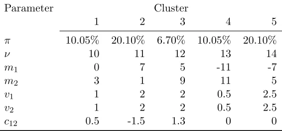
Figure 2: Misclassification rates (blue), and estimated noise proportions (red) by RIMLE

remaining clusters achieving a misclassification rate of 61.4% (i.e., the best misclassification rate that can be achieved by permutation of the cluster labels so that no cluster is identified

with the noise). Note that in this paper, mclust always automatically chooses an optimal

covariance matrix parametrization by the BIC (see Fraley et al., 2012; Celeux and Govaert, 1995). One could wonder whether the data set may be an easy job for clustering methods that take into account outliers, but this is not the case as shown in Section 7. All robust methods require tuning that, directly or indirectly, controls the amount of noise present in the data set. Perhaps the only exception is the MLE for Gaussian mixtures with uniform

noise of Banfield and Raftery (1993) implemented in the mclust package, but this can be

led astray if the noise in fact behaves very differently from a uniform distribution. In real situations a priori information on the level of the noise is rarely available. The RIMLE method treated in this paper also requires tuning. The level of the noise is essentially

controlled by the level of the improper noise density, called δ. For a given value of δ, the

noise proportion then is estimated from the data.

For the data set in Figure 1 we computed the RIMLE for several values of log(δ) (there

are other constants required, chosen as γ = 100 and πmax = 0.5, see Algorithm 2 and

Sections 3). When choosing log(δ) appropriately, namely log(δ) ∈[−53,−36], the RIMLE

gets the structure of the data set right, and it stably produces a misclassification rate in

the range [6.4%, 11%] with an estimated noise proportion in the range [34.38%,45.8%].

This is clearly better than most other robust clustering methods we tried, see Section 7.

Values of log(δ) below -100 do not change the results. For large values of log(δ) too much

noise is found, hence the RIMLE’s noise proportion constraint (see Section 3) becomes active and the resulting estimated noise proportion gets close to zero. The OTRIMLE

criterion of Coretto and Hennig (2016) selects an optimal value log(δ) =−40, which is in

the region where RIMLE shows its best performance. The RIMLE at log(δ) =−40 produces

a misclassification rate of 8.8% with estimated noise proportion equal to 44.8%. Figure 2

shows how solutions change with changing values of log(δ).

Another experimental situation considered in this paper is the GEM (“Gross Error Model”) sampling design (Figure 3). In the GEM, 100 points are sampled from two normal populations with extremely different scatters, 2 points (2%) are outliers almost lying on a hyperplane. These outliers are not extremely separated from the regular points, and this can cause trouble to robust methods. Surprisingly, in a situation like this, some non-robust methods perform better than some robust alternatives. In fact, ML for plain Gaussian

mixtures performed with mclust (without the noise component) assigns the two outliers

to cluster 1 and achieves a misclassification rate of 2%, although the estimated mixture

parameters are strongly biased. Robust methods may do worse if not well tuned (see

Section 7). As for the previous data set the RIMLE has been computed for several values of

log(δ) maintaining all other parameters as before. The result can be seen in Figure 4. For

any −∞<log(δ)≤ −46 the RIMLE is 100% accurate and estimates a noise proportion of

2%. The OTRIMLE method for the data-driven choice ofδ selects log(δ) =−200, which is

X1

−8 −4 0 2 4 6

+ + 1 1 11 1 1 1 11 1 1 11 1 11 1 1 1 11 1 1 1

2 22 2 2 2 2 2 2 2 2 22 2 2 22 2 2 2 ₂ 2 2 2 2 2 2 2 2 2 2 2 22 2 2 2 2 2 2 2 2 22 2 22 2 2 2 22 22 2 2 2 2 2 2 2 2 2 222 2 22 2 2 2 22 + + 1 1 11 1 1 1 11 1 1 1 1 111 1 1 1 11 1 1 1 2 2 2 2 2 2 2 2 2 2 2 222 2 2 2 2 2 2 2 2 2 2 2 2 2 2 2 2 2 2 2 2 2 2 2 2 2 2 2 2 2 222 2

2 2 2 22 2 2 2 2 2 2 2 2 2 2 2 2 2 22222

22 22

−5 0 5

+ + 1 1 1 1 1 1 1 1 1 1 1 1 1 1 11 1 1 1 11 1 1 1

2 22 2 2 2 2 2 2 2 2 22 2 2 2 2 2 2 2 2 2 2 2 2 2 2 2 2 2 2 2 2 2 2 2 2 2 2 2 2 22₂222

2 2 2 2 2 2 2 2 2 22 2 2 2 2 2 222

2 2 2 2 2 2 22 0 2 4 6 + + 1 1 1 1 1 1 1 1 1 1 1 1 1 1 1 1 1 1 1 11 1 1 1 2 2 2 2 2 2 2 2 2 22 2 2 2 2 2 2 2 2 2 2 2 2 2 2 2 2 2 2 2 2 2 2 2 2 2 2 2 2 2 2 22 2₂22 2 2 222 2 2 2 2 2 2 2 22 2 2 2 2 2 2 2 2 2 2 2 2 2 −8 −4 0 2 4 6 + + 1 1 1 1 1 1 1 1 1 1 1 11 1 11 1 1 1111 1 1 2 2 2 2 2 2 2 2 2 2 2 22 2 2 22 2 ₂

2 2 ₂ 2 2 2 2 2 2 2 2 2 2 2 2 2 2 2 2 2

222 2 22 2 2 2 2 2 22 22 2 2 22 2 2 2 2 2 2 22 22 2 2 22 22

X2 + + 1 11 1 1 1 1 11 1 1 1 111 1 1

1 1111 1 1 2 2 22 2 2 2 2 2 2 2 22 2 2 2 2₂2 2 2 2 2 2 22 2 2 2 2 2 2 2 2 2 2 2 2 2 22 2 2 2 2 22 2 2 2 22 2 2 2 2 2 2 22 2 2 2 2 2 2 22 2 2 2222 + + 1 11 1 1 1 1 1 11 1 1 111

1 1

1 1111

1 1

2 2 2 22 2 2 2 2 2 2 22 2 2 2 2 2 2 2 22 2 2 2 2 2 2 2 2 2 2 2 2 2 2 2 2 2 2 2 222222

2 2 2 2 2222

2 2222 2 2 2 2 22 22

2 2 2 2 22

+ + 1 11 1 1 1 1 1 1 1 1 1 1 11

1 1 1 1 1111 1 2 2 22 2 2 2 2 2 2 2 2 2 2 2 2 2 2 2 2 2 2 2 2 2 2 2 2 2 222 2222

2 2 2 2 22 2 2 22 2 2

2 2

22 22 2 2 2 2 22

2 2222 2 2 2 2 2 2 22 2 + + 1 1₁11 1

1 1 111 1111

1

1 1 1111 1 1 2 2 2 2 2 2 2 2 2 2 2 22 2 2 2

2₂2 2 2

2 2 2

2 2222₂ 2 2 22 2 2 2 2 2 222

2 2 2 2 2 2 2 2 22 2 2 2 2₂ 2 2 2 22₂ 2

2 2 2 2 22 22 2 2

+ +

1 1111 1

1 1111 1111

1

1 1 1111 1 1

2 2 222 2 222

2 2 22 2 2 2 2 22 2 2 2 2 2 2 2 2 ₂ 2 2 22 22 2 2 2 2 2 2 2 2 2 2 2 22 2 2 2 222

2 2 2 ₂ 2 2 2 2 22₂

2 2 22 2 22 222 X5 + + 1 11 1 1 1 1111 11 11 11 1 1 1111

1 1 2 2 2 2 2 2 2 2 2 2 2 22 22 2 2 22 2 2 2 2 2 2₂22

2 2 2 2 2 2 2 2 2 2 2 22 2 2 2 2 2 2₂ 2 2 2 2 2 2 2 2 2 2 2 2 2 2 2 2 2 2 222 2 2 2 2

2 −8 −4 0 2 4 6 + + 1 11 1 1 1 11 1 1 11 1 1 1 1 1 1 1 1111 1 2 2 2 22 2 22 2 2 2 2 2 2 2 2 2 2 2₂ 2

2 2 2 22₂2

2 2 2 2 2 2 2 2 2 2 22 22 2 2 2 2 2 2 2 2 22 2 2 2 2₂ 2 2 2 2 2₂2

2 2

2 2 22 222 2 −5 0 5 + + 1 1 1 1

1 1

1 1 1 1

1 1111 1 1

1 11111 1

222 2 2 2 2 2 2 2 2 22 2 2 2222 2

222 2 2 2 2 2 2 2 2 2 2 2 2 2 2 2 2 2 2 2 2 22 2 2 2₂₂ 2

2 2 2 2 2 22 2 22 2 2 2 2 22 2 2 2 22 22 + + 1 1 11₁ 1

1 11 1 1 1111

1 1

1 11111 1

222222 2222222

2 2 22 2₂ 2 2 2 2 2 2 2 2 2 2 2 2 2 2₂2 2 2 2 2 2 2 2 2 2 2 22 2 2 2 2 2 2 2 2 2 2 22 2 2 2 2 222 22 2 2₂ 22 2 + + 1 1 11₁ 1 1 111 1 1 111 1 1 1 11111 1

2 2 22 222 2

2 2222 2 2 22222 2 2 22

2 2 2 2 2 2 2 2 2 2 2 2 2 2 2222 2

2 2 22 2 2 _{2 2}2

2 2 2₂₂2 2222

2 2 2 22222₂2

22

X10

+ +

1 1 11

1 1 11 1 1 11 1 11

1 1 1 1 1111 1 2 22 2₂ 2 22 2 22 2 2 2 2 2 22 22 2 22₂2

2 2 2 2 2 2 2 2 ₂ 2 2 2 2 2 2 2 2 2 2 2_{2 2} 2 2222 2

2 2 2 2 2 2_{22 2}

22 2 2 2 2 2 2 2 22 2

0 2 4 6

+ +

1 1111

1 1 1 1 1 1 1 1 1 11 1 1 1 111 1 1 2 2 2 2 2 2 2 2 2 2 2 22 2 ₂ 2 2 2 2 2 2 2 2 2 2 2 2 2 2 2 2 2 2 2 2 2 2 2 22 2 2 2 22 22 2 2 222 2 2 2 2 2222 22 2 2 2 2 2 2 2 2 2 22 2 + + 1 1111 1 1 1 1 1 1 1 1 1 11 1 1 1 1111 1 2 2 2 22 2 2 2 2 2 2 22 2 2 2 2 2 2 2 2 2 2 2 2 2 2 22 2 22 2 2 2 2 2 2 2 2 2 2 2 2 2 22

2 2 2 2 2 2 2 2 22₂22 2 2 2 2 2 2 2 2 2 22 22 2

−8 −4 0 2 4 6

+ +

1 1111 1 1 1 11 1 1 1 11 1 1 1 11111 1 2 2 2 22 2 22 2 2 2₂₂₂ 2 2 2 2 2 2 2 22₂22222

2 2 2 2 2 2 2 2 2 22 2 2 2 2 2 22 2 2₂2 22 2

222₂2222 22 2 2 2 22 2 2 2 2 2 + +

1₁1 1 1 1 11 11 11 1 1 11 1 1 1 1111 1 2 2 2 2 2 22₂

2 2 2₂₂ 22

2 22

2 2 222 2 2 2 2 22 2 2 2 2 2 2 2 2 2 22 2 2 2 22 2 2 22 2 2 2 2 2 2 222₂2 2 2 2 2 2 2 2 2 2 2 2 22 2

−8 −4 0 2 4 6

−8 −4 0 2 4 6 X20

Figure 3: Scatter plots of n= 100 points sampled from the GEM sampling design defined

in Section 7. Marginals 1,2,5,10, and 20 are represented, further dimensions show a similar pattern. Colors denote the 2 clusters, while noise is represented by the “+” symbol. 0 5 10 15 20 25 30 35 40 45 50 Misclassif

ication rate [%]

Estimated noise proportion [%]

0 5 10 15 20 25 30 35 40 45 50

−100 −90 −80 −70 −60 −50 −40 −30 −20 −10 0 log(δ)

Figure 4: Misclassification rates (blue), and estimated noise proportions (red) by RIMLE

3. Basic definitions

In this section we define the robust improper maximum likelihood estimator (RIMLE) along with its constrained parameter space.

3.1 RIMLE and clustering

The RIMLE is based on the “noise component” idea for robustification of the MLE based on the Gaussian mixture model. This models the noise by a uniform distribution, but in fact we are interested in more general patterns of noise or outliers. However, regions of high density are rather associated with clusters than with noise, so the noise regions should be those with the lowest density. This kind of distinction can be achieved by using the uniform density as in Banfield and Raftery (1993), but in the presence of gross outliers the dependence of the uniform distribution on the convex hull of the data causes a robustness problem (Hennig (2004)). The uniform distribution is not really used here as a model for the noise, but rather as a technical device to account for whatever goes on in low density regions. The RIMLE drives this idea further by using an improper uniform distribution the density value of which does not depend on how far awy extreme points in the data are from

the main bulk. In the following, assume an observed sample x1, x2, . . . , xn,where xi is the

realization of a random variableXi∈Rp withp >1;X1, . . . , Xni.i.d. The goal is to cluster

the sample points into G distinct groups. RIMLE then maximizes a pseudo-likelihood,

which is based on the improper pseudo-density

ψδ(x, θ) =π0δ+

G

X

j=1

πjφ(x;µj,Σj), (1)

whereφ(·, µ,Σ) is the Gaussian density with meanµand covariance matrix Σ,π0, πj ∈[0,1]

for j= 1,2, . . . , G, π0 +

PG

i=1πj = 1, while δ is the improper constant density. The

pa-rameter vectorθcontains all Gaussian parameters plus all proportion parameters including

π0, ie. θ= (µ1, . . . , µG,vect(Σ1), . . . ,vect(ΣG), π0, . . . , πG),where vect(A) is the vectorized

upper (or lower) triangle including the main diagonal of the symmetric square matrixA. δ

and the number of Gaussian componentsGare considered fixed and known. Although this

does not define a proper probability model, it yields a useful procedure for data modelled

as a proportion of (1−π0) of a mixture of Gaussian distributions, which have high enough

density peaks to be interpreted as clusters plus a proportion π0 times something

unspec-ified with density smaller than or equal to δ (which may even contain further Gaussian

components with so few points and/or so large within-component variation that they are not considered as “clusters”). The definition of the pseudo-model in (1) requires that the

value of δ is fixed in advance. The choice of δ will be discussed in Section 5.2.

Given the sample improper pseudo-log-likelihood function

ln(θ) =

1

n n

X

i=1

logψδ(xi, θ), (2)

the RIMLE is defined as

θn(δ) = arg max

θ∈Θn

where Θn is a constrained parameter space defined in Section 3.2. θn(δ) is then used to

cluster points using pseudo posterior probabilities for belonging to the Gaussian components or the improper uniform. These pseudo posterior probabilities are given by

τj(xi, θ) :=

( _π

0δ

ψδ(xi,θ) ifj = 0

πjφ(xi,µj,Σj)

ψδ(xi,θ) ifj = 1,2, . . . , G;

fori= 1,2, . . . , n.

Points are assigned to the component for which the pseudo posterior probability is maxi-mized. The assignment rule is then given by

J(xi, θ) := arg max

j∈{0,1,2,...,G}

τj(xi, θ). (4)

The assignment based on maximum posterior probabilities is common to all model-based clustering methods. Here, an improper density is involved, and so these are “pseudo poste-rior probabilities”.

We also define a population version of the RIMLE for later deriving consistency results

for the sequence{θn(δ)}n∈_N. Let EPf(x) be the expectation off(x) underP. The RIMLE

population target function and the constrained parameter set can be obtained by replacing

the empirical measure withP, and the population version ofln(θ) is given by

L(θ) = EPlog(ψδ(x, θ)).

Define LG = supθ∈ΘG(P)L(θ), where ΘG(P) is a constrained parameter space defined in

Section 3.2.

3.2 The constrained parameter space

Some notation: thekth element ofµjis denoted byµj,kfork= 1,2, . . . , pandj= 1,2, . . . , G.

Letλj,k be the kth eigenvalue of Σj, define Λ(θ) ={λj,k: j= 1,2, . . . , G; k= 1,2, . . . , p},

λmin(θ) = minj,k{Λ(θ)},λmax(θ) = maxj,k{Λ(θ)}.

Remark 1 The p-dimensional Gaussian density can be written in terms of the eigen-de-composition of the covariance matrix:

φ(x;µ,Σ) = (2π)−p2

p

Y

k=1

λk

!−1₂

exp −1

2

p

X

k=1

λ−_k1(x−µ)0vkvk0(x−µ)

!

,

whereλk is thek-th eigenvalue ofΣ, andvk is its associated eigenvector, fork= 1,2, . . . , p.

Let λ0 = min{λk; k= 1,2, . . . , p}. Then, limλ0&0φ(µ;µ,Σ) = ∞, with φ(µ;µ,Σ) =

O(λ−₀p/2) as λ0 & 0. On the other hand limλ0&0φ(x;µ,Σ) = 0 for all x 6= µ, with

φ(x;µ,Σ) =o(λ₀q) for any fixed q as λ0 &0. This implies that

lim

λ0&0

φ(µ;µ,Σ)φ(x;µ,Σ)→0 for anyx6=µ

Furthermore, each of the density components in ψδ(·) can be bounded above in terms of λmax(θ) andλmin(θ):

φ(x;µj,Σj)≤(2πλmin(θ))−

p

2 exp

−1

2λmax(θ)

−1_kx−µ

jk2

≤(2πλmin(θ))−

p

The optimization problem in (3) requires that Θn is suitably defined, otherwise θn(δ) may

not exist. Consider a sequence (θm)m∈N, as discovered by Kiefer and Wolfowitz (1956), the

likelihood of a Gaussian mixtures degenerates ifλ1,1,m&0 ifµ1,m=x1, and this holds for

(2), too. We here use the eigenratio constraint

λmax(θ)/λmin(θ)≤γ <+∞ (6)

with a constant γ ≥ 1, where γ = 1 constrains all component covariance matrices to be

spherical and equal, as ink-means clustering. This type of constraint has been proposed by

Jr (1981), while Hathaway (1985) showed consistency of the scale-ratio constrained MLE for one-dimensional Gaussian mixtures. Ingrassia (2004) and Ingrassia and Rocci (2007) introduced EM algorithms for implementing these constraints for multivariate datasets. TCLUST by Garc´ıa-Escudero et al. (2008) and Garc´ıa-Escudero et al. (2014) also makes use of eigenratio constraints. Moreover there are a number of alternative constraints, see Ingrassia and Rocci (2011); Gallegos and Ritter (2009). It may be seen as a disadvantage of (6) that the resulting estimator will not be affine equivariant (this would require allowing

λmax(θ)/λmin(θ) → ∞ within any component). Affine equivariance can be achieved by

defining a sphered version of the RIMLE as

θ∗_n(δ) =θ_n∗(δ, x1, . . . , xn) =θn(δ, x∗1, x∗2, . . . , x∗n)

withx∗_i =A(xi−m), i= 1, . . . , n, whereS(x1, . . . , xn)−1 =A0A;S(x1, . . . , xn) could be the

sample covariance matrix or another scale matrix andmthe mean vector or another location

estimator. This yields affine equivariance because the sphered versions of{x1, . . . , xn} and

{Bx1+b, . . . , Bxn+b}with some invertiblep×p-matrixB andb∈Rp are the same. Affine equivariance is not necessarily desirable though, see Hennig (2015a), Sec. 31.3.4.

This defines the parameter space

˜ Θ :=







θ: πj ≥0∀j ≥1, π0+

G

X

j=1

πj = 1;

λmax(θ) λmin(θ)

≤γ







. (7)

Occasionally, later, the notationkθk will refer to the Euclidean norm of a vector pieced

to-gether from all the parameters collected inθ, in which all covariance matrices are interpreted

as subvectors of all the matrix entries.

Although (6) ensures the boundedness of the likelihood in standard mixture models and TCLUST, for RIMLE this is not enough. The Gaussian components could degenerate on a few points and all other points could be fitted by the improper uniform component. Therefore we impose an additional constraint:

1

n n

X

i=1

τ0(xi, θ)≤πmax, (8)

for fixed 0< πmax<1. The quantityn−1Pn_i=1τ0(xi, θ) can be interpreted as the estimated

proportion of noise points. This constraint depends on the dataset. Unfortunately the

similar looking constraint π0 ≤ πmax independent of the data will not do, because this

could not stop more than a portion of π0 points to be fitted by the improper uniform

There is therefore a constrained effective parameter space for RIMLE estimation de-pending on the dataset:

Θn:=







θ∈Θ :˜ πj ≥0∀j≥1, π0+

G

X

j=1

πj = 1;

1

n n

X

i=1

τ0(xi, θ)≤πmax;

λmax(θ) λmin(θ)

≤γ







.

(9) Analogously, existence and consistency of the RIMLE functional can only be showed on a

parameter subset of ˜Θ that depends on the underlying distribution and enforces that enough

probability mass is fitted by Gaussian components rather than the improper uniform:

ΘG(P) :=







θ∈Θ :˜ πj ≥0∀j≥1; π0+

G

X

j=1

πj = 1; EP

π0δ ψδ(x, θ)

≤πmax;

λmax(θ) λmin(θ)

≤γ







.

(10)

4. RIMLE existence and consistency

We first show existence of the RIMLE for finite samples Let #(A) denote the cardinality

of the set A. Let xn = {x1, x2, . . . , xn}. Lemma 2 concerns the important case of plain

Gaussian mixtures (δ = 0) and requires a weaker assumption A0(a) for existence than A0

required for the RIMLE withδ >0. Here are some assumptions:

A0(a) #(xn)> G.

A0 #(xn)> G+dnπmaxe.

Lemma 2 Assume A0(a),δ = 0. Let(θm)m∈N be a sequence such thatλmax(θm)/λmin(θm)

≤γ. Assume also that for somej = 1,2, . . . , G andk= 1,2, . . . , p,λk,j,m &0 as m→ ∞; thensupln(θm)→ −∞.

Proof λk,j,m & 0 implies λmax(θm) & 0, λmin(θm) & 0 at the same speed because of

(6). Assume w.l.o.g. (otherwise consider a suitable subsequence) that (θm)m∈_N is such

that µj,m, j = 1,2, . . . , G either leave every compact set for m large enough or converge,

and assume w.l.o.g., that if their limits are in {x1, . . . , xn}, they are inxG={x1, . . . , xG}.

A0(a) implies that∃xi 6∈xG, and∃ν >0 such that for all suchxi, j= 1,2, . . . , Gand large

enoughm:kxi−µj,mk ≥ν. Because the likelihood

L_n(θm) =

Y

xi∈xG

nXG

j=1

πjφ(xi;µj,m,Σj,m)

o Y

xi6∈xG

nXG

j=1

πjφ(xi;µj,m,Σj,m)

o

, (11)

and Remark 1, the first product is of orderO(λmin(θm)−p/2)G, and the second one of order

o(λmin(θm)q) for any fixedq, which implies that Ln(θm)→0 andln(θm)→ −∞.

Proof Using the definitions of the proof of Lemma 2, instead of (11) now

Ln(θm) =

Y

xi∈xG

n

π0,mδ+ G

X

j=1

πjφ(xi;µj,m,Σj,m)

o _Y

xi6∈xG

n

π0,mδ+ G

X

j=1

πjφ(xi;µj,m,Σj,m)

o

(12)

has to be considered, so that the limit behaviour of (π0,m)m∈N is relevant. (8) implies

1

n

X

xi∈xG



1 +

G

X

j=1

πjφ(xi, µj,m,Σj,m) π0,mδ





−1

+1

n

X

xi6∈xG



1 +

G

X

j=1

πjφ(xi, µj,m,Σj,m) π0,mδ





−1

≤πmax.

(13)

Suppose that (π0,m)m∈_N does not converge to zero as O(φ(xi, µj,m,Σj,m)) for at least one

xi 6∈ xG. For m → ∞, the left term of (13) is ≥0, and the right term (at least a

subse-quence) converges to #(xn_n\xG), which A0 requires to be > πmax with contradiction, thus

π0,m = O(φ(xi, xj,Σj,m)). Therefore, by the same argument as in the proof of Lemma 2,

the right product in (12) vanishes fast enough so thatln(θm)→ −∞.

From these Lemmas:

Theorem 4 (Finite Sample Existence) Assume A0. Thenθn(δ) exists for allδ ≥0.

Proof Θn depends onδ via (8). Θn is not empty for anyδ, because for any fixed values of

the other parameters, small enoughπ0 will fulfil (8). Next show that there exists a compact

set Kn⊂Θn such that supθ∈Knln(θ) = supθ∈Θnln(θ).

Step A:considerθsuch thatπ1 = 1,µ1=x1, Σj =Ipfor allj= 1,2, . . . , G, arbitraryµj and

πj = 0 for allj 6= 1. For this, ln(θ) =

Pn

i=1logφ(xi;x1,Σ1) >−∞, thus supθ∈Θnln(θ) >

−∞.

Step B: consider a sequence ( ˙θm)m∈N. It needs to be proved that if ( ˙θm)m∈N leaves a

suitably chosen compact set Kn, it cannot achieve as large values of ln as one could find

within Kn. Lemma 3 (Lemma 2 for δ= 0) rules out the possibility of anyλk,j,m&0.

Step C: (5) implies thatln(θ) can be bounded from above in terms ofπ0, λmin andδ:

ln(θ) =

1

n n

X

i=1

log 

π₀δ+

G

X

j=1

πjφ(xi;µj,Σj)



≤log

π0δ+ (1−π0)(2πλmin(θ))−

p

2

.

Consider ˙θ ∈ Θn such that ˙λk,j < +∞ for all k= 1,2, . . . , p and j = 1,2, . . . , G (using

the obvious notation of components of “dotted” parameter vectors). Also consider a

se-quence (¨θm)m∈N such that ¨θm → θ¨ where ¨θ is equal to ˙θ except that ¨λk,j,m → +∞ for

some k ∈ {1, . . . , p} and j ∈ {1, . . . , G}. By (6), λmin(¨θm) → +∞ and thus ln(¨θm) →

log(¨π0δ). Clearly ¨π0 <1 because otherwisen−1Pn_i=1τ0(xi,θ¨) = 1, violating (8). Therefore

limm→∞ln(¨θm)≤ln( ˙θ).

Step D: now consider ||µ˙j,m|| → +∞, for j = 1, w.l.o.g. Choose ¨θm equal to ˙θm except

now ¨µ1,m= 0 for all m. Note that φ(xi; ˙µ1,m,Σ˙1)→0 for all i= 1,2, . . . , n, which implies

this argument to all j with ||µ˙j,m|| → +∞ shows that better ln can be achieved inside a

compact set.

Continuity of ln now guarantees existence of θn(δ).

We now derive consistency for the sequence{θn(δ)}n∈_Nas estimator ofLG. Consistency

of the RIMLE can be achieved only if LG exists. In order to ease the notation we define

η(x, θ) =PG

j=1πjφ(x;µj,Σj).Consider the following assumptions onP:

A1 For everyx1, . . . , xG∈Rp :P{x1, . . . , xG}<1−πmax.

A2 LG> LG−1, where for G∈Nlet LG= supθ∈ΘG(P)L(θ).

A3 There exist1, 2>0 so that for every θwith π0 < 1:L(θ)≤LG−2.

Remark 5 Assumption A1 requires that no set of G points carries probability 1−πmax

or more. Otherwise the log-likelihood can be driven to ∞ by fittingG mixture components to G points with all covariance matrix eigenvalues converging to zero. The improper noise component could take care of all other points.

Note that assumptions A2 and A3 are not both required, but only any single one of them. A2 states that G mixture components fit the data better than G−1 components. If this is not the case, there is at least one redundant component, and one cannot make sure thatL(θ)

is bounded away from LG for large n in some distance from the “true” RIMLE-functional as the redundant component can be moved around, see Theorem 11. In case that A2 is not fulfilled, a weaker result can still be achieved, namely the existence of a not necessarily unique consistent sequence of local maximizers of ln. This requires A3, which states that a noise proportion bounded away from zero is required for maximizing L. If neither A2 nor A3 are fulfilled,P can be fitted perfectly by fewer thanGmixture components and no noise. In this case one cannot stop the remaining mixture components from leaving every compact set, and therefore one cannot expect consistency of all components for any method; as long as there is still noise bounded away from zero, those mixture components still can contribute to fitting what otherwise would be noise, and fits become worse if these degenerate.

Note that this is less often the case than one might expect; for example, a plain Gaussian mixture withG−1components may still fulfill A3: if the density of one of the components is uniformly smaller than δ, a better pseudo-likelihood can obviously be achieved by assigning its proportion to the noise component than by choosingπ0 =πG= 0 and otherwise the true parameters. A Gaussian component that “looks like noise” rather than like a “cluster” will be treated as noise.

Lemma 6 For any probability measure P onRp, LG >−∞.

Proof Choose compactK⊂_Rp_{withP(K)>0. Letq = 1−P(K) and chooseKbig enough}

thatπmax> q. Chooseµ1= EP(x|x∈K), Σ1= CovP(x|x∈K), π2 =. . .=πG = 0. If all

eigenvalues of Σ1 are zero, choose Σ1 =Ip. Let λmax,1 be the largest eigenvalue of Σ1. If

thanγλmax,1 byγλmax,1 in its spectral decomposition. Letφmin= minx∈Kφ(x, µ1,Σ1)>0.

Choose

π0=

(πmax−q)φmin

2((1−πmax)δ+ (πmax−q)φmin)

>0, π1= 1−π0.

Observe that the resulting θ∈ΘG(P) (with all other parameters chosen arbitrarily) by

EP

π0δ ψδ(x, θ)

= Z

K

π0δ π0δ+η(x, θ)

dP(x) + Z

Kc

π0δ π0δ+η(x, θ)

dP(x)≤

≤(1−q) π0δ

π0δ+ (1−π0)φmin

+q.

This is smaller than πmax if π0 < _(1−πmax(πmax_)c+(−_πq_max)φmin_−q)φ

min. Furthermore, L(θ) ≥ (1−

q) log(π0δ+ (1−π0)φmin) +qlog(π0δ)>−∞.

Lemma 7 Assume A1. There are λ∗_min>0, λ∗_max<∞, >0, so that

(a) L(θ)≤LG−for everyθ with λmin(θ)< λ∗min or λmax(θ)> λ∗max,

(b) for x1, x2, . . . i.i.d. with L(x1) = P, for sequences (θn)n∈N with λmin(θn) < λ ∗ min or λmax(θn)> λ∗max for large enough n: ln(θn)≤ln(θn(δ))−a.s.

Proof Start with part (a). First consider a sequence{θm}m∈N∈ΘG(P)

N_withλ

max(θm)→

∞. The eigenvalue ratio constraint forces all covariance matrix eigenvalues to infinity, and

therefore sup_xφ(x, µj,m,Σj,m) & 0. But this means that EP_ψδπ₍0_x,θδ ₎ → 1 > πmax and

θm 6∈ ΘG(P) eventually, unless π0,m & 0, too. If the latter is the case, ψδ(x, θ) & 0

uniformly over allx and L(θm)& −∞, which together with Lemma 6 makes it impossible

thatL(θm) is close toLG form large enough andλmax(θm) too large, proving the existence

of the upper boundλ∗_max<∞ as required.

Now consider a sequence {θm}_m∈_N∈ΘG(P)N with λmin(θm)→0. Define

Am,=

x: min

j=1,2,...,Gkx−µj,mk>

.

A1 ensures that for 0< 3 there exists > 0 so that for all m∈N:P(Am,) ≥πmax+3.

Based on (5) derive an upper bound for π0,m from the constraint

R π0,mδ

π0,mδ+η(x,θm)dP(x) ≤

πmax:

Z

π0,mδ π0,mδ+η(x, θm)

dP(x) = Z

Am,

π0,mδ π0,mδ+η(x, θm)

dP(x) + Z

Ac

m,

π0,mδ π0,mδ+η(x, θm)

dP(x)≥

≥P(Am,)

π0,mδ

π0,mδ+ maxx∈Am,η(x, θm)

,

which by (5) implies

π0,m≤

πmaxmaxx∈Am,η(x, θm)

δ(P(Am,)−πmax)

≤ πmaxexp(−

2

2γλmin(θm))

For the log-likelihood,

L(θm) =

Z

Am,

log(π0,mδ+η(x, θm))dP(x) +

Z

Ac

m,

log(π0,mδ+η(x, θm))dP(x)≤

≤ Z

Am,

log 



δπmaxexp(−

2

2γλmin(θm))

δ3(2π)p/2λmin(θm)p/2

+ exp(

−_2γλ 2

min(θm))

(2π)p/2_λ

min(θm)p/2



dP(x)+

+ Z

Ac

m, log





δπmaxexp(−

2

2γλmin(θm))

δ3(2π)p/2λmin(θm)p/2

+ 1

(2π)p/2_λ

min(θm)p/2



dP(x)≤

≤P(Am,)

− c1

λmin(θm)

−c2log(λmin(θm)) +c3

+

+P(Ac_m,) (o(1)−c4log(λmin(θm)) +c5) =

=− c6

λmin(θm)

−c7log(λmin(θm)) +c8

for positive constants c1, c2, c4, c6, c7 and constants c3, c5, c8, all independent of θm. If

λmin(θm)&0, this implies L(θm)& −∞, proving together with Lemma 6 the existence of

the lower boundλ∗_min>0.

Part (b) holds because if (θm)m∈_N is chosen as above form=n→ ∞ andP is replaced

by the empirical distribution Pn, Glivenko-Cantelli enforces Pn(An,)−P(An,) → 0 a.s.

Glivenko-Cantelli applies because the class of allAn, is a subset of the class of intersections

of the complements of all closed balls, and therefore a Vapnik-Chervonenkis class, see van der Vaart and Wellner (1996). The argument carries over using all other integrals in the finite

sample-form, i.e., w.r.t. Pn. Lemma 6 carries over becauseln(θ)→L(θ) a.s. by the strong

law of large numbers forθ withL(θ)>−∞.

Remark 8 Lemma 7 (a) and (5) imply that for all θ with L(θ)> LG−, j= 1,2, . . . , G and all x:

φ(x, µj,Σj)≤φmax=

1 (2π)p/2_(λ∗

min)p/2 .

This implies LG<∞.

The same holds because of Lemma 7 (b) for x1, x2, . . . i.i.d. with L(x1) = P for large

enough na.s. for all θ with ln(θ)> ln(θn(δ))−.

Lemma 9 Assume A1 and A2. There is a compact set K ⊂_Rp _{so that}

(a) L reaches its supremum for µ1, . . . , µG ∈K and is bounded away from the supremum if not all ofµ1, . . . , µG∈K (i.e., ∃4>0so thatL in this case is bounded from above

by supL−4),

Proof Start with part (a). Consider a sequence{θm}m∈N∈ΘG(P)

N_withkµ

jmk → ∞for

j= 1, . . . , k, 1≤k < Gand a compact setK withµjm∈K forj > k. Let

Am =

(

x: ∀j∈ {1, . . . , k}:φ(x, µj,m,Σj,m)≤m G

X

l=k+1

πl,mφ(x, µl,m,Σl,m)

)

,

where m & 0 slowly enough that P(Am) → 1. Let πm∗ =

Pk

j=1πj,m. Let θ(G−k),m for

m∈_N be defined byπ0,(G−k),m =π0,m, π(j−k),(G−k),m=πj,m(1−π0,m)(1−πm∗ −π0,m)−1

for j = k+ 1, . . . , G accompanied by the µj,Σj-parameters belonging to the components k+ 1, . . . , G of θm. Observe, using Remark 8,

L(θm) =

Z

Am

log(ψδ(x, θm))dP(x) +

Z

Ac

m

log(ψδ(x, θm))dP(x)≤

≤ Z

Am

log((1 +m)ψδ(x, θ(G−k)m))dP(x) +P(Acm) log(δ+φmax)

implying L(θ(G−k)m)−L(θm) → 0. EP[π0,(G−k),mδ(ψδ(x, θ(G−k)m))−1]≤ πmax will be

ful-filled for m large enough because it is fulfilled for θm by definition and ψδ(x, θ(G−k),m) >

ψδ(x, θm) on Am withP(Am)→1. L(θ(G−k)m)< LG−1 implies that, because of A2, θm is

bounded away fromLG.

Regarding existence of a maximum with µ1, . . . , µG ∈K, observe that with Remark 8,

ψδ(x, θ) can be bounded by δ +φmax for all θ for which L(θ) > LG−. Now consider

a sequence (θm)m∈_N so that ∀m : µ1m, . . . , µGm ∈ K, with the notation of Lemma 7,

λ∗_min≤λmin(θm)≤λmax(θm)≤λ∗max and L(θm)→LG. Because of compactness, w.l.o.g.,

θm → θ+ and, using Fatou’s Lemma, LG = limm→∞L(θm) ≤ EPlim supmψδ(x, θm) =

L(θ+)≤LG.

Part (b) holds because if (θm)m∈_N is chosen as above form=n→ ∞ andP is replaced

by the empirical distribution Pn, Glivenko-Cantelli enforces Pn(An) −P(An) → 0 a.s.

Glivenko-Cantelli applies here because a sequence of closed balls (Bn)n∈Ncan be constructed

so that Bn ⊆An, P(Bn) → 1 a.s.; the closed balls are a Vapnik-Chervonenkis class, and

Pn(An) ≥Pn(Bn)→ 1 a.s. Furthermore, for θ∈ ΘG(P) with L(θ)> LG−1: ln(θ)→ L(θ)

a.s. by the strong law of large numbers, so that for large enoughn: sup_θ∈ΘG(P)ln(θ)> LG−1

a.s. On the other hand, θ_(G−k),n can be chosen optimally in a compact set K because of

Lemma 7, within which ln converges uniformly toL a.s. (Theorem 2 in Jennrich (1969)),

and therefore, lim sup_n→∞ln(θ(G−k),n) ≤ LG−1. With these ingredients, the argument of

part (a) carries over.

Lemma 10 Assume A1 and A3. There is a compact set K⊂Rp so that

(a) L reaches its supremum for µ1, . . . , µG∈K,

Proof Start with part (a). Consider a sequence {θm}m∈N ∈ ΘG(P)

N _{with kµ}

j,mk → ∞

for j = 1, . . . , k, 1 ≤ k < G (the case k = G is treated at the end), and a compact set

K with µj,m ∈ K for j > k. By selecting a subsequence if necessary, assume that there

existsµj = limm→∞µj,m,Σj = limm→∞Σj,m fork+ 1≤j ≤Gand thatπj,m converge for

j = 0, . . . , G. Let j∗ = arg max

k+1≤j≤G

EPφ(x, µj,Σj). Suppose L(θm) % LG monotonically and,

by A3, assume π0,m> 1.

Consider first the case Pk

j=1πj,m → 3 >0. Construct another sequence {θ∗m}m∈N ∈

ΘG(P)N for which µ1,∗m =. . . =µk,∗m =µj∗ ∈K, Σ_1,∗m = . . .= Σ_k,∗m = Σ_j∗. All other

parameters are the same as in θm. Let Am = {x: ∀j∈ {1, . . . , k} : 2φ(x, µj,m,Σj,m) ≤

φ(x, µj∗,Σ_j∗)}. Observe P(A_m)→1. Now

L(θ∗m)−L(θm) =

Z

Am

logψδ(x, θ∗m)

ψδ(x, θm)

dP(x) + Z

Ac

m

logψδ(x, θ∗m)

ψδ(x, θm)

dP(x). (14)

For large enough m,

Z

Am

logψδ(x, θ∗m)

ψδ(x, θm)

dP(x)≥5>0,

whereas (using Remark 8)

Z

Ac

m

logψδ(x, θ∗m)

ψδ(x, θm)

dP(x)≥P(Ac_m) log 1δ

δ+φmax

→0. (15)

Therefore L(θ∗m)−L(θm) >0 for large enough m so thatL(θm) is improved by a θ with

µj ∈K forj= 1,2, . . . , G.

Consider now Pk

j=1πjm →0. Construct another sequence {θ∗m}m∈N∈ΘG(P)

N _{for which}

µ1,∗m = . . . = µk,∗m = µj∗ ∈ K, Σ_1,∗m = . . . = Σ_k,∗m = Σ_j∗, π_1∗m = . . . = π_k∗m = 0, π0∗m =

Pk

j=0πjm, all other parameters taken from θm. Set Am ={x : ∀j ∈ {1, . . . , k} :

φ(x, µjm,Σjm)< δ}. AgainP(Am)→1. With this, (14) holds again. This time

Z

Am

logψδ(x, θ∗m)

ψδ(x, θm)

dP(x)>0

and again (15).

Letθ∗ = limm→∞θ∗m(this exists by construction). Continuity ofLimplies thatL(θ∗) =

LGand therefore for allm:L(θ∗)≥L(θm). Pk_j=1πj,m→0 is required here becauseπ0,∗m≥

π0,m does not necessarily fulfill EP_ψδπ₍0_x,θ,∗m_∗mc₎ ≤ πmax, but limm→∞π0,∗m = limm→∞π0,m

does.

Finally, considerk=G. WithAm,={x: ∀j∈ {1, . . . , k}:φ(x, µj,m,Σj,m)< δ}, observe

EP

π0,mδ ψδ(x, θm)

≥P(Am,)

π0,mδ π0,m(c+)

> πmax,

for small enough and large enoughm, violating for largem the corresponding constraint

in ΘG(P) as long as π0,mis bounded from below, as was assumed. Existence follows in the

same way as in the proof of Lemma 9.

For part (b) let θ∗ have µ∗₁, . . . , µ∗_G ∈K and L(θ∗) = LG, which exists because of part

of large numbers yields ln(θ∗) → LG a.s., and Theorem 2 of Jennrich (1969) implies that

for all sequences (θn)n∈N∈(K

∗_{)N: lim sup}

n→∞ln(θn)≤LG. This also holds for sequences

(θn)n∈N that are eventually outside K

∗ _{because of part (a) of Lemma 7 and the proof of}

part (a) above, because if (θm)m∈_N is chosen as above for m= n→ ∞ and P is replaced

by the empirical distribution Pn, Glivenko-Cantelli (which applies by the same argument

as used in the proof of Lemma 9) enforcesPn(An)−P(An)→0 a.s., which means that as

in part (a), a.s., eventuallyln(θn) cannot converge to anything larger thanLG.

Theorem 11 (RIMLE existence) Assume A1 and any one of A2 or A3. There is a compact subset K⊂ΘG(P) so that there existsθ∈K : ∞> L(θ) =LG>−∞. Assuming A2, for θ6∈K, L(θ) is bounded away from LG.

Proof Pieced together from Lemmas 6-9 parts (a) and Remark 8. Theorem 11 establishes existence of the RIMLE functional

θ?(δ) = arg max

θ∈ΘG(P)

L(θ). (16)

Unfortunately neither L(θ) nor ln(θ) can be expected to have a unique maximum. If we

take the vector θ and we permute some of the triples (πj, µj,Σj) we still obtain the same

value forL(θ) andln(θ). This known as “label switching” in the mixture literature. There

could be other causes for multiple maxima. Without strong restrictions on P, we cannot

identify any specific source of multiple optima in the target function. Instead we show that asymptotically the sequence of estimators is close to some maximum of the pseudo-loglikelihood, which amounts to consistency of the RIMLE with respect to a quotient space

topology identifying all loglikelihood maxima, as done in Redner (1981). By θ?_{(δ) in (16)}

we mean any of the maximizer of L(θ). Define the sets

S( ˙θ) =

θ∈ΘG(P) :

Z

logψδ(x;θ)dP(x) =

Z

logψδ(x; ˙θ)dP(x)

,

K( ˙θ, ε) =nθ∈ΘG(P) :kθ−θ¨k< ε∀θ¨∈S( ˙θ)

o

, for any ε >0.

The following theorem makes a stronger statement assuming A2 than A3, because if A2

does not hold, the Gth mixture component is asymptotically not needed and cannot be

controlled for finite noutside a compact set.

Theorem 12 (Consistency) Assume A1 and A2. Then for every ε > 0 and every se-quence of maximizers θn(δ) of ln:

lim

n→∞P{θn(δ)∈ K(θ

?_{(δ), ε)}= 1.}

Assuming A3 instead of A2, for every compact K ⊃ K(θ?_{(δ), ε) there exists a sequence of} θn that maximize ln locally in K so that

lim

n→∞P{θn∈ K(θ

Proof Under A2, because of the parts (b) of the Lemmas 7 and 9 it can be assumed

that there is a compact set K so that all θn(δ) ∈ K for large enough n a.s. Under A3,

considerations are restricted to K anyway.

Based on Theorem 11 and related Lemmas |logψδ(x, θ)| ≤C for some finite constant

C for allθ∈K. Sufficient conditions for Theorem 2 in Jennrich (1969) are satisfied, which

implies uniform convergence of ln(θ), that is supθ∈K|ln(θ)−L(θ)| → 0 P-a.s. Based on

the latter, and applying the same argument as in proof of Theorem 5.7 in van der Vaart

(2000), it holds true that L(θn(δ))→ L(θ?(δ))P-a.s. By continuity of L(θ) and Theorem

11 we have that for every ε > 0 there exists a β > 0 such that L(θ?(δ))−L(θ) > β for

all θ ∈ K\ K(θ?(δ), ε). Denote (Ω,A, P) the probability space where the sample random

variables are defined and consider the following events

An={ω∈Ω : θn(δ)∈K\ K(θ?(δ), ε)},

and

Bn={ω ∈Ω : L(θ?(δ))−L(θn(δ))> β}.

Clearly An⊆ Bn for all n. P(Bn) → 0 forn → ∞ implies P(An)→ 0. The latter proves

the result.

5. Algorithms and practical issues

Following the presentation of the proposed algorithm to compute the RIMLE, we discuss its initialization and tuning.

5.1 RIMLE computing

In this section we develop Expectation–Maximization type algorithms (EM) to compute the

RIMLE (for a fixed δ ). Lets= 0,1, . . . be the iteration index. Let a(s+1) be the quantity

acomputed at the sth step of the EM algorithm. Define

Q(θ, θ(s)) =

n

X

i=1

G

X

j=0

τj(xi, θ(s)) logπj+ n

X

i=1

τ0(xi, θ(s)) logδ+

+

n

X

i=1

G

X

j=1

τj(xi, θ(s)) logφ(xi;µj,Σj). (17)

Increasing (17) by an appropriate choice of θ increases ln(·). An approximate candidate

maximum ofln(θ) can be found by the EM Algorithm 1.

Proposition 13 Assume A0. The sequence {θ(s)}s∈N produced by Algorithm 1 converges

to a point θem_n ∈Θ, and ln(θ(s)) is increased in every step.

Proof Find a set An⊂Rp that contains all points inxnwith Lebesgue measure M(An) =

1/δ. δ is then a proper uniform density function on An. Hence, for a given dataset the