Learning Parts-Based Representations of Data

Learning Parts-Based Representations of Data

David A. Ross [email protected]

Richard S. Zemel [email protected]

Department of Computer Science University of Toronto

6 King’s College Road

Toronto, Ontario M5S 3H5, CANADA

Editor: Pietro Perona

Abstract

Many perceptual models and theories hinge on treating objects as a collection of constituent parts. When applying these approaches to data, a fundamental problem arises: how can we determine what are the parts? We attack this problem using learning, proposing a form of generative latent factor model, in which each data dimension is allowed to select a different factor or part as its expla-nation. This approach permits a range of variations that posit different models for the appearance of a part. Here we provide the details for two such models: a discrete and a continuous one. Further, we show that this latent factor model can be extended hierarchically to account for correlations between the appearances of different parts. This permits modeling of data consisting of multiple categories, and learning these categories simultaneously with the parts when they are unobserved. Experiments demonstrate the ability to learn parts-based representations, and categories, of facial images and user-preference data.

Keywords: parts, unsupervised learning, latent factor models, collaborative filtering, hierarchical

learning

1. Introduction

Many collections of data exhibit a common underlying structure: they consist of a number of parts or factors, each with a range of possible states. When data are represented as vectors, parts manifest themselves as subsets of the data dimensions that take on values in a coordinated fashion. In the domain of digital images, these parts may correspond to the intuitive notion of the component parts of objects, such as the arms, legs, torso, and head of the human body. Prominent theories of compu-tational vision, such as Biederman’s Recognition-by-Components (Biederman, 1987) advocate the suitability of a parts-based approach for recognition in both humans and machines. Recognizing an object by first recognizing its constituent parts, then validating their geometric configuration has several advantages:

1. Highly articulate objects, such as the human body, are able to appear in a wide range of configurations. It would be difficult to learn a holistic model capturing all of these variants.

3. The appearances of certain parts may vary less under a change in pose than the appearance of the whole object. This can result in detectors which, for example, are more robust to rotations of the target object.

4. New examples from an object class may be recognized as simply a novel combination of familiar parts. For example a parts-based face detection system could generalize to detect faces with both beards and sunglasses, having been trained only on faces containing one, but not both, of these features.

The principal difficulty in creating such systems is determining which parts should be used, and identifying examples of these parts in the training data.

In the part-based detectors created by Mohan et al. (2001) and Heisele et al. (2000) parts were chosen by the experimenters based on intuition, and the component-detectors—support vec-tor machines—were trained on image subwindows containing only the part in question. Obtaining these subwindows required that they be manually extracted from hundreds or thousands of train-ing images. In contrast, the parts-based detector created by Weber et al. (2000) proposed a way to automate this process. During training of the geometric model, parts were selected from an initial set of candidates to include only those which lead to the highest detection performance. The re-sulting detector relied on a very small number of parts (e.g., 3) corresponding to very small local features. Unlike the SVMs, which were trained on a range of appearances of the part, each of these part-detectors could identify only a single fixed appearance.

Parts-based representations of data can also be learned in an entirely unsupervised fashion. These parts can be used for subsequent supervised learning, but the models constructed can also be valuable on their own. A parts-based model provides an efficient, distributed representation, and can aid in the discovery of causal structure within data. For example, a model consisting of K parts, each with J possible states, can represent JK different objects. Inferring the state of each part can be done efficiently, as each part depends only on a fraction of the data dimensions.

These computational considerations make parts-based models particularly suitable for modeling high-dimensional data such as user preferences in collaborative filtering problems. In this setting, each data vector contains ratings given by a human subject to a number of items, such as books or movies. Typically there are thousands of unique items, but for each user we can only observe ratings for a small fraction of them. The goal in collaborative filtering is to make accurate predictions of the unobserved ratings. Parts can be formed from groups of related items, and the states of a part correspond to different attitudes towards the items. Unsupervised learning of a parts-based model allows us to learn the relationships between items, which allows for efficient online and active learning.

Here we propose a probabilistic generative approach to learning parts-based representations of high-dimensional data. Our key assumption is that the dimensions of the data can be separated into several disjoint subsets, or factors, which take on values independently of each other. Each factor has a range of possible states or appearances, and we investigate two ways of modeling this variability. First we address the case in which each factor has a small number of discrete states, and model it using a vector quantizer. In some situations, however, continually-varying descriptions of parts are more suitable. Thus, in our second approach we model part-appearances using factor

analysis. Given a set of training examples, our approach learns the association of data dimensions

Section 2. Experiments showing parts-based representations learned for real data sets follow in Section 3.

Although we initially assume that parts take on states independently, clearly in real-world situ-ations there are dependencies. For example, consider the case of modeling images of human faces. A model could be constructed representing the various parts of the face (eyes, nose, mouth, etc.), and the various appearances of each part. If one part were to select an appearance with high pixel intensities, due to lighting conditions or skin tone, then it seems likely that the other parts should appear similarly bright. Realizing this, in Section 4 we propose a method of learning these depen-dencies between part selections hierarchically, by introducing an additional higher-level cause, or ‘class’ variable, on which state selections for the factors are conditioned. This allows us to model different categories of data using the same vocabulary of parts, and to induce the categories when they are not available in advance. We conclude with a comparison to related methods, and a final discussion in Sections 5 and 6.

2. An Approach to Learning Parts-Based Models

We approach the problem of learning parts by posing it as a stochastic generative model. We assume that there are K factors, each a probabilistic model for the range of appearances of one of the parts. To generate an observed data vector of D dimensions, x∈ℜD_{, we stochastically select one state} for each factor, and one factor for each data dimension, xd. The first selection allows each part to independently choose its appearance, while the second dictates how the parts combine to produce the observed data vector.

This approach differs from a traditional mixture model in that each dimension of the data is gen-erated by a different linear combination of the factors. Rather than clustering the data vectors based on which mixture component gives the highest probability, we are grouping the data dimensions based on which part provides the best explanation.

The selection of factors for each dimension are represented as binary latent variables, R={rdk}, for d =1...D,k=1...K. The variable rdk=1 if and only if factor k has been selected for data dimension d. These variables can be described equivalently as multinomials, rd∈1...K, and are drawn according to their respective prior distributions, P(rdk) =adk. The choice of state for each factor is also a latent variable, which we will represent by sk. Usingθkto represent the parameters of the kthfactor, we arrive at the following complete likelihood function:

P(x,R,S|θ) =

∏

d,k

(adkrdk)

∏

k

(P(sk))

∏

d,k

(P(xd|θk,sk)rdk). (1)

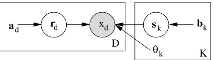
This probability model is depicted graphically in Figure 1.

As described thus far, the approach is independent of the particular choice of model used for each of the factors. We now provide details for two particular choices: a discrete model of factors, vector quantization; and a continuous model, factor analysis.

2.1 Multiple Cause Vector Quantization

x_d

d

a rd sk bk

θ_k D

K

Figure 1: Graphical representation of the parts-based learning model. We let rd=1represent all the variables rd=1,k, which together select a factor for x1. Similarly, sk=1 selects a state for factor 1. The plates depict repetitions across the D input dimensions and the K factors. To extend this model to multiple data cases, we would include an additional plate over r,

x, and s.

VQ, and, as described above, one VQ for each dimension. Given these selections, a single state from a single VQ determines the value of each data dimension xd.

As before, we represent the selections using binary latent variables, S={sk j}, for k=1...K,j= 1...J, where sk j=1 if and only if state j is selected for VQ k. Again we introduce prior selection probabilities P(sk j) =bk j, with∑jbk j=1.

Assuming each VQ state specifies the mean as well as the standard deviation of a Gaussian distribution, and the noise in the data dimensions is conditionally independent, we have (where θk={µdk j,σdk j}, and

N

is the Gaussian pdf)

P(x|R,S,θ) =

∏

d,k,j

N

(xd; µdk j,σ2dk j)rdksk j.

The resulting model can be thought of as a Gaussian mixture model over J×K possible states

for each data dimension (xd). The single state k j is selected if sk jrdk=1. Note that this selection has two components. The selection in the j component is made jointly for the different data dimensions, and in the k component it is made independently for each dimension.

2.1.1 LEARNING ANDINFERENCE

The joint distribution over the observed vector x and the latent variables is

P(x,R,S|θ) = P(R|θ)P(S|θ)P(x|R,S,θ),

=

∏

d,k

ardk

dk

∏

k,j

bs_{k j}k j

∏

d,k,j

N

(xd;θk)rdksk j.

Given an input x, the posterior distribution over the latent variables, P(R,S|x,θ), cannot tractably be computed, since all the latent variables become dependent.

We apply a variational EM algorithm to learn the parametersθ, and infer latent variables given observations. For a given observation, we could approximate the posterior distribution using a factored distribution, where g and m are variational parameters related to r and s respectively:

Q0(R,S|x,θ) =

∏

d,k

grdk

dk

∏

k,j

msk j

k j

The model is learned by optimizing the following objective function (Neal and Hinton, 1998), also known as the variational free energy:

F

(Q0,θ) = EQ0[log P(x,R,S|θ)−log Q0(R,S|x,θk)],

= EQ0 "

−

∑

d,k

rdklog(gdk/adk)−

∑

k,j

sk jlog(mk j/bk j) +

∑

d,k,j

rdksk jlog

N

(xd;θ)

#

,

= −

∑

d,k

gdklog

gdk

adk −

∑

k,j

mk jlog

mk j

bk j −

∑

d,k,j

gdkmk jεdk j,

whereεdk j=logσdk j+

(xd−µdk j)2

2σ2

dk j

. The objective function

F

is a lower bound on the log likelihood of generating the observations, given the particular model parameters. The variational EM algorithm improves this bound by iteratively maximizing

F

with respect to Q0(E-step) and toθ(M-step).

Extending this to handle multiple observations—the columns of X= [x1. . .xC]—we must now consider approximating the posterior P(

R

,

S

|X,θ), where

R

={r_dkc }and

S

={sc_{k j}}are the latent selections for all training cases c. Our aim is to learn models which have a posterior distribution over factor selections for each data dimension that is consistent across all data (that is to say, regardless of the data case, each xd will typically be associated with the same part or parts). Thus, in the variational posterior we constrain the parameters{gdk}to be the same across all observations xc,c= 1. . .C. In this general case, the variational approximation to the posterior becomes (cf. Equation (2))

Q(

R

,

S

|X,θ) =

∏

c,d,k

gdkr

c dk

∏

c,k,j

mc_{k j}sck j

. (3)

It is important to point out that this choice of variational approximation is somewhat unorthodox, nonetheless it is perfectly valid and has produced good results in practice. A comparison to more conventional alternatives appears in Appendix A.

Under this formulation, only the{mc_{k j}}parameters are updated during the E step for each ob-servation xc:

mc_{k j}=bk jexp

−

∑

d

gdkεcdk j

/

J

∑

ρ=1

bkρexp

−

∑

d

gdkεcdρk

.

The M step updates the parameters, µ and σ, which relate each latent state k j to each input dimension d, the parameters of Q related to factor selection{gdk}, and the priors{adk}and{bk j}:

gdk=adkexp

−1

C

∑

_c,jm

c k jεcdk j

/

K

∑

ρ=1

adρexp

−1

C

∑

_c,jm

c jρεcd jρ

, (4)

µdk j=

∑cmck jxcd ∑cmck j

, σ2_{dk j}=∑cm

c

k j(xcd−µdk j)2 ∑cmck j

,

adk=gdk, bk j=

1

C

∑

_c m

c k j.

A variational approximation is just one of a number of possible approaches to performing the intractable inference (E) step in MCVQ. One alternative, known as Monte Carlo EM, is to approxi-mate the posterior with a set of samples {

R

n,

S

n}Nn=1 drawn from the true posterior P(

R

,

S

|X,θ) via Gibbs sampling. The M step now becomes a maximization of the approximate likelihood

1

N∑nP(X,

R

n,

S

n|θ) with respect to the model parameters θ. Note that the intractable marginal-ization over{rc_dk,sc_{k j}} has been replaced with the less-costly sum over N samples. Details of this approach for a related model can be found in Ghahramani (1995), and a general description in Andrieu et al. (2003).

2.2 Multiple Cause Factor Analysis

In MCVQ, each factor is modeled as a set of basis vectors, one of which is chosen at a time when generating data. A more general approach is to allow data to be generated by arbitrary linear com-binations of the basis vectors in each factor. This extension (with the appropriate choice of prior distribution) amounts to modeling the range of appearances for each part with a factor analyzer.

A factor analysis (FA) model (e.g., Ghahramani and Hinton, 1996) proposes that the data vectors come from a low-dimensional linear subspace, represented by the basis vectors of the factor loading

matrix,Λ∈ℜD×J_{, and an offset}

ρ∈ℜDfrom the origin. A data vector is produced by taking a linear

combination s∈ℜJ_{of the columns ofΛ. The linear combination is treated as an unobserved latent} variable, with a standard Gaussian prior P(s) =

N

(s; 0,I). To this is added zero-mean Gaussian noise, independent along each dimension. The probability model is

P(x,s|θ) =

N

(x;Λs+ρ,Ψ)

N

(s; 0,I) (5)

whereΨis a D×D diagonal covariance matrix.

As with MCVQ, we assume that the data contains K parts and model each using a factor analyzer θk= (Λk,ρk,Ψk). A data vector is again generated by stochastically selecting one state skper factor

k, and choosing one factor per data dimension. Under this model factor analyzer k proposes that the

value of xdhas a Gaussian distribution centered atΛk_dsk+ρdkwith varianceΨk_d(whereΛk_dindicates the dth row of factor loading matrix k, and Ψk_d the dth entry on the diagonal of Ψk). Thus the likelihood is

P(x|R,S,θ) =

∏

d,k

N

(xd;Λkdsk+ρdk,Ψkd)rdk.

2.2.1 LEARNING ANDINFERENCE

Again this model produces an intractable posterior over latent variables S and R, so we resort to a variational approximation:

Q(

R

,

S

|X,θ) =

∏

c,d,k

gr

c dk

dk

∏

c,k

N

(sc_k; mc_k,Ωck).

for the E-step:1

mc_k=ΩckΛkTΨ−1k ((x c₋

ρk).∗gk),

Ωck=

ΛkT gk ΨkΛ

k_+I−1_{, hs}c

ksckTi=Ωck+mckmckT,

where gk

Ψk is a diagonal matrix with entries gdk/Ψk_d. Note that the expression forΩckis independent

of the index over training cases, c, thus we need only have oneΩk=Ωck,∀c.

The M-step involves updating the prior and variational posterior factor-selection parameters, {adk}and{gdk}, as well as the parameters(Λk,ρk,Ψk) of each factor analyzer. At each iteration the prior, adk=gdkis set to the posterior at the previous iteration. The remaining updates are

gdk∝

adk |Ψk

d|1/2 exp

−1 2CΨk

d

∑

c

(x_dc−ρdk)2+ΛdkhscksckTiΛkd T

−2(xc_d−ρdk)Λkdmck

,

Λk_{= X−}

ρk1T

MT_k

∑

c

hsc_ksc_kTi

−1

,

ρk= 1

C

∑

_c

xc−Λk_mc k , Ψk d= 1

C

∑

_c

(xc_d−ρdk)2+Λkdhscksck T_iΛk

d T

−2(xc_d−ρdk)Λkdmck

.

where (Mkis a J×C matrix in which the cthcolumn is mc_k).

2.3 Related Algorithms

Here we present the details of two related algorithms, principal components analysis (PCA), and non-negative matrix factorization (NMF). A more detailed comparison of these algorithms with MCVQ and MCFA appears below, in Section 5.

The goal of PCA is to learn a factorization of the data matrix X into the product of a coefficient matrix S and an orthogonal basisΛso that X≈ΛS. TypicallyΛhas fewer columns than rows, so S can be thought of as a reduced-dimensionality approximation of X, andΛas the key features of the data. Using a squared-error cost function, the optimal solution is to letΛbe the top eigenvectors of the sample covariance matrix, _C−11 XXT_{, and let S=}ΛT_X.

PCA can also be posed as a probabilistic generative model, closely related to factor analysis (Roweis, 1997; Tipping and Bishop, 1999). In fact, probabilistic PCA proposes the same generative model, Equation (5), except that the noise covariance,Ψ, is restricted to be a scalar times the identity matrix:Ψ=σ2_I.

Non-negative matrix factorization (Lee and Seung, 1999) also learns a factorization X≈WH

of the data matrix, but includes the additional restriction that X, W, and H must be entirely non-negative. By allowing only additive combinations of a non-negative basis, Lee & Seung propose to obtain basis vectors that correspond to the intuitive parts of the data. Instead of squared error, NMF seeks to minimize the divergence D(XkWH) =∑d,c

xc_dlog(WH)dc−(WH)dc

which is the

1. The second uncentered momenthsc_ksc_kTineed not be computed explicitly, since it can be expressed as a combination of the first and second centered moments, mk andΩck. It is, however, a useful subexpression for computing the

negative log-probability of the data, assuming a Poisson density function with mean WH. A local minimum of the divergence is obtained by iterating the following multiplicative updates:

wd j←wd j

∑

c

xc_d (WH)dc

hjc, wd j←

wd j

∑d0w_d0_j, hjc←hjc

∑

d

wd j

xc_d (WH)dc

.

Despite the probabilistic interpretation, X∼Poisson(WH), NMF is not a proper probabilistic generative model, since it does not specify a prior distribution over the latent variable H. Thus NMF does not specify how new data could be generated from a learned basis.

Like the above methods, MCVQ and MCFA can be viewed as matrix factorization methods, where the left-hand matrix is formed from the {gdk} and the collection of VQ/FA basis vectors, while the right-hand matrix is comprised of the latent variables{mc_{k j}}. This view highlights the key contrast between the assumptions about the data embodied in these earlier models, as opposed to the proposed model. Here the data is viewed as a concatenation of components or parts, corresponding to particular subsets of data dimensions, each of which is modeled as a convex combination of appearances.

3. Experiments

In this section we examine the ability of MCVQ and MCFA to learn parts-based representations of data from two different problem domains.

We begin by modeling sets of digital images, in this case images of human faces. The parts learned are fixed subsets of the data dimensions (pixels), corresponding to fixed regions of the images, that closely resemble intuitive notions of the parts of faces. The ability to learn parts is robust to partial occlusions in the training images.

The application of MCVQ and MCFA to image data assumes that the images are normalized, that is, that the head is in a similar pose in each image, and aligned with respect to position and scale. This constraint is standard for learning methods that attempt to learn visual features beyond low level edges and corners, though, if desired, the model could be extended to perform automatic alignment of images (Jojic and Caspi, 2004). While normalization may require a preprocessing step for image applications, in many other types of applications, the input representation is more stable. For instance, in collaborative filtering each data vector consists of a single user’s ratings for a fixed set of items; each data dimension always corresponds to the same item.

Thus, we also explore the application of MCVQ and MCFA to the problem of predicting ratings of unseen movies, given observed ratings for a large set of users. Here parts correspond to subsets of the movies which have correlated ratings.

Code implementing MCVQ and MCFA in MATLAB, as used for the following experiments, can be obtained at http://www.cs.toronto.edu/∼dross/mcvq/.

3.1 Face Images

The face data set consisted of 2429 images from the CBCL Face database #1 (MIT-CBCL, 2000). Each image contained a single frontal or near-frontal face, depicted in 19×19 pixel grayscale. The images were histogram equalized, and pixel values rescaled to lie in[−2,2]. Sample training images are shown in Figure 2.

Figure 2: Sample training images from the CBCL Face database #1.

VQ 1

VQ 2

VQ 3

VQ 4

VQ 5

VQ 6

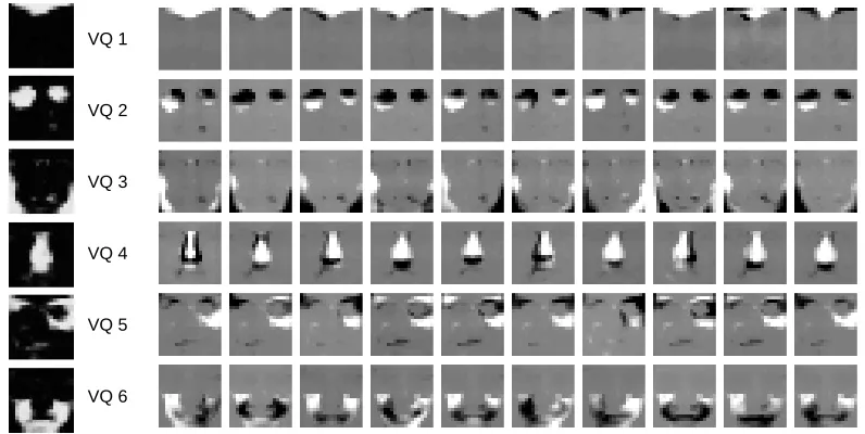
Figure 3: The parts-based model of faces learned by MCVQ. On the left are plots showing the posterior probability with which each pixel selects the indicated VQ. On the right are the means, for each state of each VQ, masked by the aforementioned selection probabilities (µk j.∗gk).

the MCFA model with J=4 basis vectors converged in 15 variational EM iterations. In practice, the Monte Carlo approach to inference leads to better local maxima of the objective function, and better parts-based models of the data. For both MCVQ and MCFA, prior probabilities were initialized to uniform, and states/basis vectors to randomly selected training images. The learned parts-based decompositions are depicted in Figures 3 and 4.

On the left of each figure is a plot of posterior probabilities {gdk}that each pixel selects the indicated factor as its explanation. White indicates high probability of selection, and black low. As can be seen, each gkcan be thought of as a mask indicating which pixels ‘belong’ to factor k.

In the noise-free case, each image generated by one of these models is a sum of the contributions from the various factors, where each contribution is ‘masked’ by the probability of pixel selection. For example in Figure 3 the probability of selecting VQ #4 is non-zero only around the nose, thus the contribution of this VQ to the remaining areas of the face in any generated image is negligible.

On the right of each figure is a plot of the 10 states/4 basis vectors for each factor. Each image has been masked (via element-wise multiplication) with the corresponding gk. For MCVQ this is

FA 1

FA 2

FA 3

FA 4

FA 5

FA 6

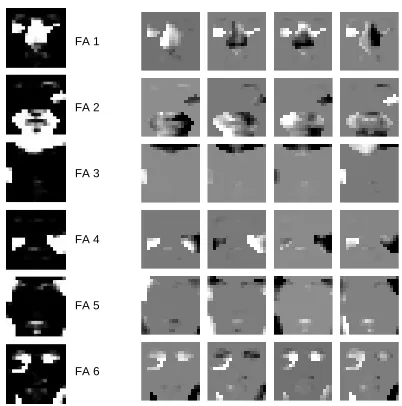
Figure 4: The parts-based model of faces learned by MCFA.

when generating a face. These range from thin to wide, with shadows of the left or right, and with light or dark upper-lips (possibly corresponding to moustaches). In MCFA, on the other hand, the basis vectors are not discrete alternatives. Rather these vectors are combined via arbitrary linear combinations to generate an appearance of a part.

To test the fidelity of the learned representations, the trained models were used to probabilisti-cally classify held-out test images as either face or non-face. The test data consisted of the 472 face images and 472 randomly-selected non-face images from the CBCL database test set. To classify test images, we evaluated their probability under the model, labeling an image as face if its prob-ability exceeded a threshold, and non-face if it did not. For each model the threshold was chosen to maximize classification performance. Evaluating the probability of a data vector under MCVQ and MCFA can be difficult, since it requires marginalizing over all possible values of the latent vari-ables. Thus, in practice, we use a Monte Carlo approximation, obtained by averaging over a sample of possible selections. The results of this experiment are shown in Table 1. In addition to MCVQ and MCFA, we performed the same experiment with four other probabilistic models: probabilistic principal components analysis (PPCA), mixture of Gaussians, a single Gaussian distribution, and cooperative vector quantization (Hinton and Zemel, 1994) (which is described further in Section 5). It is important to note that in this experiment an increase in model size (using more VQs, states, or basis vectors) does not necessarily improve the ability to discriminate faces from non-faces. For example, PPCA achieves its highest accuracy when using only three basis vectors, and a mixture of Gaussians with 60 states outperforms one with 84 states. As can be seen, the highest performance is achieved by an MCVQ model with 6 VQs and 14 states per VQ.

Model Accuracy MCVQ (6 VQs, 14 states each) 0.8305

Mixture of Gaussians (60 states) 0.8072 MCVQ (6 VQs, 10 states each) 0.8030 Probabilistic PCA (3 components) 0.7903 Gaussian distribution (diagonal covariance) 0.7871 Mixture of Gaussians (84 states) 0.7680 MCFA (6 FAs, 3 basis vectors each) 0.7415 MCFA (6 FAs, 4 basis vectors each) 0.7267 Cooperative Vector Quantization (6 VQs, 10 states each) 0.6208

Table 1: Results of classifying test images as face or non-face, by computing their probabilities under trained generative models of faces.

Figure 5: Synthetic images generated using MCVQ (left) and MCFA (right).

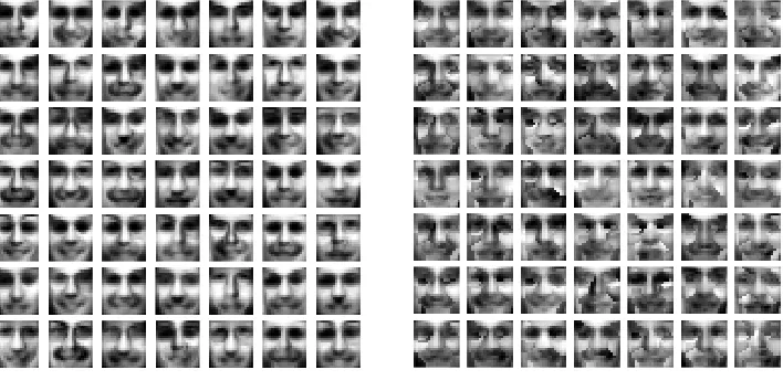
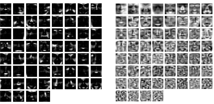
The parts-based models learned by MCVQ and MCFA differ from those learned by NMF and PCA, as depicted in Figure 6, in two important ways. First, the basis is sparse—each factor con-tributes to only a limited region of the image, whereas in NMF and PCA basis vectors include more global effects. Secondly MCVQ and MCFA learn a grouping of vectors into related parts, by explicitly modeling the sparsity via the gdkdistributions.

Figure 6: Bases learned by non-negative matrix factorization (left) and probabilistic principal com-ponents analysis (right), when trained on the face images.

3.1.1 PARTIALOCCLUSION

Parts-based models can also be reliably learned from image data in which the object is partially occluded. As an illustration, we trained an MCVQ model on a data set containing partially-occluded faces. The occlusions were generated by replacing pixels in randomly-selected contiguous regions of each training image with noise. The noise, which covered 1₄ to 1₂ of each image, had the same first- and second-order statistics as the unoccluded pixels. The resulting training set contained 4858 images, half of which were partially occluded.

Examples of the training images, and the resulting model, can be seen in Figure 7. In the model each VQ has learned at least one state containing a blurry region, which corresponds to an occluded view of the respective part (e.g., for VQ 1, the second state from the right). Thus this model is able to generate and reconstruct (recognize) partially-occluded faces.

3.2 Collaborative Filtering

Here we test MCVQ on a collaborative filtering task, using the EachMovie data set, where the input vectors are ratings by viewers of movies, and a given element always corresponds to the same movie. The original data set contains ratings, on a scale from 1 to 6, of a set of 1649 movies, by 74,424 viewers. In order to reduce the sparseness of the data set, since many viewers rated only a few movies, we only included viewers who rated at least 20 movies, and removed unrated movies. The remaining data set, containing 1623 movies and 36,656 viewers, was still very sparse (95.7%).

VQ 1

VQ 2

VQ 3

VQ 4

VQ 5

VQ 6

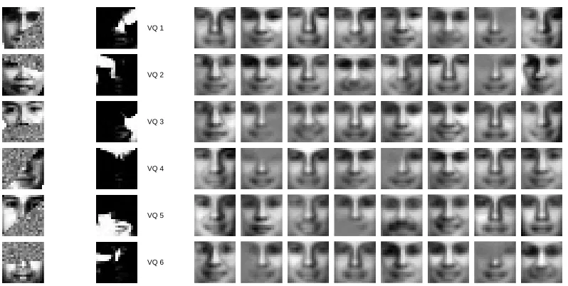
Figure 7: The model learned by MCVQ on partially-occluded faces. On the left are six representa-tive images from the training data. In the middle are plots of the posterior part selection probability (the gdk’s) for each VQ. On the right are the (unmasked) means for each state of each VQ. Note that each VQ has learned at least one state to represent partial occlusion of the corresponding part.

of 2/3 of the viewers, with the remaining 1/3 viewers retained as a testing set.2 _{This model was used} to predict the held-out ratings of the training viewers, a task referred to as weak generalization, as well as the held-out ratings of the testing viewers, called strong generalization. Each prediction was obtained by first inferring the latent states of the factors mk j, then averaging the mean of each state by its probability of selection:∑k,jgdkmk jµk jd.

Prediction performance was calculated using normalized mean absolute error (NMAE). Given a set of predictions{pi}, and the corresponding ratings{ri}, the NMAE is

1

zn

n

∑

i=1

|ri−pi|

where z is a normalizing factor equal to the expectation of the mean absolute error, assuming uniformly distributed pi’s and ri’s (Marlin, 2004).3 For the EachMovie data set this value is

z=35/18≈1.9444.

We trained several models on this data set, including MCVQ, MCFA, factor analysis, mixture of Gaussians, as well as a baseline algorithm which, for each movie, simply predicts the mean of

2. This differs slightly from Marlin’s approach. He used three randomly sampled training and test sets of 30000 and 5000 viewers respectively. However, his test sets were not disjoint, introducing a potential bias in the error estimate. We, instead, partitioned the data into thirds, using 2/3 of the viewers for training and 1/3 for testing in each of the three folds. The resulting estimates of error should be less biased, but remain directly comparable to Marlin’s results. 3. For data sets in which the ratings range over the integers, from a minimum of m to a maximum of M, there is a simple

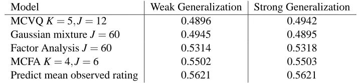
Model Weak Generalization Strong Generalization

MCVQ K=5,J=12 0.4896 0.4942

Gaussian mixture J=60 0.4945 0.4895 Factor Analysis J=60 0.5314 0.5318

MCFA K=4,J=6 0.5502 0.5503

Predict mean observed rating 0.5621 0.5621

Table 2: Collaborative filtering performance. For each algorithm we show the prediction error, in terms of NMAE (see text), on held out ratings from the training data (weak generalization) and the test data (strong generalization). K and J give the number of factors and basis vectors per factor respectively.

the observed ratings for that movie. MCVQ and MCFA were both trained using variational EM, converging in 15 iterations. We selected this approach due to its efficiency, as running each of these algorithms on the large data sets used in these experiments via the Monte Carlo EM approach would require considerable computation time. Note that in the graphical model (Fig. 1), all the observation dimensions are leaves, so a data variable whose value is not specified in a particular observation vector will not play a role in inference or learning. This makes inference and learning with sparse data rapid and efficient in MCVQ and MCFA.

The results of rating prediction are summarized in Table 2 For each model, we have included the best performance, under the restriction that JK≤60. For comparison, the current state-of-the-art performance on this experiment is 0.4422 weak and 0.4557 strong generalization, by Marlin’s User Rating Profile model (Marlin, 2004).

In addition to its utility for rating prediction, the parts-based model learned by MCVQ can also provide key insights regarding the relationships between the movies. These relationships are largely captured by the learned{gdk}parameters. For a movie d, the probability distribution gd=

[gd1. . .gdK]indicates the affinity of the movie for each of the K factors. To study these relationships we retrained MCVQ on the EachMovie set, using all available data, again with K=5 and J=12.

When trained on the full data set, the average entropy of the gd distributions was only 0.0475 bits. In other words, for 98% of the movies, at least one factor was consistently selected with a posterior probability exceeding 0.9. The movies in the training set were distributed fairly evenly amongst the available factors. Specifically, using a probability of gdk>0.9 to indicate strong asso-ciation, VQs 1 to 5 were assigned 14%, 33%, 9%, 20% and 22% respectively of the movies. Thus MCVQ learned a partitioning of the movies into approximately disjoint subsets.

In the parts-based model, movies with related ratings were associated with the same factor. For example, all seven movies from the Amityville Horror series were assigned to VQ #1. Similarly the three original Star Wars movies, as well as seven of the eight Star Trek movies were all associated with VQ #5. By examining VQ #5 in more detail we can see that each state of the VQ corresponds to a different attitude towards the associated movies, or ‘ratings profile’. In Figure 8 we compare the ratings given to the Star Wars and Star Trek movies by various states of VQ #5. For each state we have plotted the difference between the predicted rating and the mean rating, µdk j−∑j0(µ_{dk j}0/J),

The four states depicted in Figure 8 show a range of possible ratings profiles. State 2 shows a strong preference for all the movies, with each receiving a rating 1-2.5 points higher than usual. In contrast, state 9 shows an equally strong dislike for the movies. State 10 indicates a viewer who is fond of Star Wars, but not Star Trek. Finally, state 11 shows an ambivalent attitude: slight preference for some films, and slight dislike for others.

W1 W2 W3 T1 T2 T3 T4 T5 T6 T7 −2.5

0 2.5

VQ 5, State 2

W1 W2 W3 T1 T2 T3 T4 T5 T6 T7 −2.5

0 2.5

VQ 5, State 9

W1 W2 W3 T1 T2 T3 T4 T5 T6 T7 −2.5

0 2.5

VQ 5, State 10

W1 W2 W3 T1 T2 T3 T4 T5 T6 T7 −2.5

0 2.5

VQ 5, State 11

Star Wars W1 Star Trek III: The Search for Spock T3 The Empire Strikes Back W2 Star Trek IV: The Voyage Home T4 Return of the Jedi W3 Star Trek V: The Final Frontier T5 Star Trek: The Motion Picture T1 Star Trek VI: The Undiscovered Country T6 Star Trek II: The Wrath of Khan T2 Star Trek: First Contact T7

Figure 8: Ratings profiles learned by MCVQ on the EachMovie data, for Star Wars and Star Trek movies. Each state represents a different attitude towards the movies. Positive scores correspond to above-average ratings for the movie, and negative to below-average.

3.2.1 ACTIVELEARNING

value could simply be the system’s certainty as to the viewer’s preferences, or, more interestingly, its ability to recommend movies that he might enjoy.

The parts based models we describe significantly simplify both of these computations. By learning a partitioning of the items, a new rating will only affect beliefs about unobserved ratings associated with the same factor. Specifically, only one mk jwill be updated for each new rating, and the update will depend only on a fraction of the observations.

Also, since we explicitly model the relationships between items, we can determine how the possible responses to a putative query would affect predictions. Thus, we can formulate a query designed to identify movies with high predicted ratings. More details on a successful application of MCVQ to active collaborative filtering, using these ideas, can be found in Boutilier et al. (2003).

4. Hierarchical Learning

Thus far it has been assumed that the states of each factor are selected independently. Although this assumption has proven useful, it is unrealistic to suppose that, for example, the appearance of the eyes and mouth in a face are entirely uncorrelated. Rather than simply being a violation of our modeling assumptions, these correlations can be viewed as an additional source of information from which we can learn higher-order structure present in the data.

Here we relax the assumption of independence by including an additional higher-level latent variable upon which state selections are conditioned. This variable has two possible interpretations. First, if the higher-level cause is unobserved, it can be learned, inducing a categorization of the data vectors based on their state selections. Secondly, if the variable is observed, it can be treated as side information available during learning. In this case the prior over state selections will be adapted to account for the side information.

We now develop both approaches, and demonstrate their use on a set of images containing different facial expressions.

4.1 Extending the Generative Model

Suppose that each data vector comes from one of N different classes. We assume that for a given data vector the selections of the states for each factor (the sk’s) depend on the class, but that the selections of a factor per data dimension (the rd’s) do not. Specifically, for training case x, we introduce a new multinomial variable y which selects exactly one of the N classes. y can be thought of as an indicator vector y∈ {0,1}N_{, where y}

n=1 if and only if class n has been selected. Using a prior P(yn=1) =βnover y, the complete likelihood takes the following form (cf. Equation (1)):

P(x,R,S,y|θ) = P(x|R,S,θ)P(R)P(S|y)P(y),

=

∏

d,k

(P(xd|θk,sk)rdk)

∏

d,k

ardk

dk

∏

n,k,j

bsk jyn

nk j

∏

n

(βyn

n). (6)

The graphical model representation is given in Figure 9.

β x_d

d

a rd sk

θ_k D

K

y

Figure 9: Graphical model with additional class variable, y. Note that y can be either observed or unobserved.

If the class variable y corresponds to an observed label for each data vector, then the new model can be thought of as a standard MCVQ or MCFA model, but with the requirement that we learn a different prior over S for each class. On the other hand, if y is unobserved, then the new model learns a mixture over the space of possible priors for S, rather than the single maximum likelihood point estimate learned in standard MCVQ and MCFA.

Below we derive the EM updates for the hierarchical MCVQ model. The derivation of hierar-chical MCFA is similar.

4.2 Unsupervised Case

In the unsupervised case, yc_{, for each training case c=1. . .C is an unobserved variable, like R}c and Sc. As in standard MCVQ, the posterior P(R,S,y|x,θ)over latent variables cannot tractably be computed. Instead, we use the following factorized variational approximation:

Q(

R

,

S

,

Y

) =

∏

c,d,k

gr c dk dk

∏

c,n,k,j

mc_{nk j}sck jycn

∏

c,n

zc_nycn

.

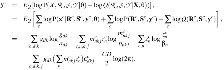
Note that, as in standard MCVQ, we restrict the posterior selections of VQ made for each training case to be identical, that is,{gdk}is independent of c. Using the variational posterior and the likelihood, Equation (6), we obtain the following lower bound on the log-likelihood:

F

= EQ[log P(

X

,

R

,

S

,

Y

|θ)−log Q(

R

,

S

,

Y

|X,θ))],

= EQ

∑

c

log P(xc|Rc,Sc,yc,θ) +

∑

c

log P(Rc,Sc,yc)−

∑

c

log Q(Rc,Sc,yc)

,

= −

∑

c,d,k

gdklog

gdk

adk −

∑

c,n,k,j

mc_{nk j}zc_nlogm c nk j

bnk j −

∑

c,n

zc_nlogz c n βn

−

∑

c,d,k,j

gdk

∑

n

mc_{nk j}zc_nεc_{dk j}−CD

2 log(2π).

By differentiating

F

with respect to each of the parameters and latent variables, and solving for their respective maxima, we obtain the EM updates used for learning the model. The E-step updates for mc_{nk j}and zc_nare

mc_{nk j}∝bnk jexp

−

∑

d

gdkεcdk j

zc_n∝ βnexp

∑

k j

mc_{nk j}logbnk j

mc_{nk j}−

∑

_{dk j}gdkm

c nk jεcdk j

.

The M-step updates for adk,gdk,µdk j,andσdk jare unchanged from standard MCVQ, except for the substitution of∑_n(mc_{nk j}zc_n)in place of mc_{k j}, wherever it appears. The updates forβnand bnk jare

βn= 1

C

∑

_c z

c

n, bnk j=

∑cmcnk jzcn ∑czcn

.

A useful interpretation of the latent variable y is that, for a given data vector, it indicates the assignment of that datum to one of N clusters. Specifically, zc_n can be thought of as the posterior probability that example c belongs to cluster n.

4.3 Supervised Case

In the supervised case, we are given a set of labeled training data(xc,yc)for c=1. . .C. Note that

this case is essentially the same as the unsupervised case—we can obtain the supervised updates by constraining zc=yc,∀c. Since the class is known, we may now drop the subscript n from mc_{nk j}.

As stated earlier, when the y’s are given, we learn a different prior over state selections for each class n:

bnk j= 1

Cβn

∑

_c

mc_{k j}yc_n,

where the prior probability of observing class n,βn, can be calculated from the training labels:

βn= 1

C

∑

_c y

c n.

The posterior probabilities of state selection for each example c, mc_{k j}, depend only on the prior corresponding to c’s class:

mc_{k j}∝byc_{k j}exp

−

∑

d

gdkεcdk j

.

4.4 Experiments

In this section we present experimental results obtained by training the above models on images taken from the AR Face Database (Martinez and Benavente, 1998). This data consists of images of frontal faces of 126 subjects under a number of different conditions. The five conditions used for these experiments were: 1) anger, 2) neutral, 3) scream, 4) smile, and 5) sunglasses.

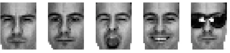
The data set in its raw form contains faces which, although roughly centered, appear at different locations, angles, and scales. Since the learning algorithms do not attempt to compensate for these differences, we manually aligned each face such that the eyes always appeared in the same location. Next we cropped the images tightly around the face, and subsampled to reduce the size to 29×22 pixels. Finally, we converted the image data to grayscale, with pixel values ranging from -1 to 1. Examples of the preprocessed images can be seen in Figure 10.

Figure 10: Examples of preprocessed images from the AR Face Database. These images, from left to right, correspond to the conditions: anger, neutral, scream, smile, and sunglasses.

4.4.1 SUPERVISEDCASE: LEARNING CLASS-CONDITIONAL PRIORS

We first trained a supervised model on the entire data set, with a goal of learning a different prior over state selections for each of the five classes of image (anger, neutral, scream, smile, and sun-glasses).

The model consisted of 5 VQs, 10 states each. The image regions that each VQ learned to explain are shown in Figure 11. For each VQ k we have plotted, as a grayscale image, the prior probability of each pixel selecting k (i.e., adk, d=pixel index). Two regions which we expected to be class discriminative, the mouth and the eyes, were captured by VQs 3 and 4 respectively.

VQ 1 VQ 2 VQ 3 VQ 4 VQ 5

Figure 11: Image regions explained by each VQ. The prior probability of a VQ being selected for each pixel is plotted as a gray value between 0=black and 1=white.

The priors over state selection for these VQs varied widely depending on the class of the image being considered. As an example, in Figure 12 we have plotted the prior probability, given the class, of selecting each of the states from VQ 3. In the figure we can see that the prior probabilities closely matched our intuition as to which mouth shapes corresponded to which facial expressions. For example the first state (top left) appears to depict a smiling mouth. Accordingly, the smile class assigned it the highest prior probability, 0.34, while the other classes each assigned it 0.05 or less. Also, given the scream class, we see that the highest prior probabilities were assigned to the third and fourth states—both widely screaming mouths. States 6 through 9 (second row) range from depicting a neutral to an angry mouth.

A N S M G 0

0.4

A N S M G 0

0.4

A N S M G 0

0.4

A N S M G 0

0.4

A N S M G 0

0.4

A N S M G 0

0.4

A N S M G 0

0.4

A N S M G 0

0.4

A N S M G 0

0.4

A N S M G 0

0.4

One method for qualitatively evaluating the suitability of a class-conditional prior is to use it to generate novel images from the model, and see how well they match the class. Samples drawn this way using each of the five priors can be seen in Figure 13.

Anger Neutral Scream Smile Glasses

Figure 13: Sample images generated from the supervised hierarchical MCVQ model. Four images are depicted for each of the five class-conditional priors. Note the generated images can contain a novel combination of parts not seen in the training data, such as a person screaming and wearing glasses (Scream, upper-left). (The images do not include the Gaussian noise described in the generative process.)

4.4.2 UNSUPERVISEDCASE

To evaluate the performance of the unsupervised model, we trained a model on a subset of the five classes, with the hope that it would learn clusters corresponding to the original classes.

The data set was restricted to contain only three classes—neutral, scream, and sunglasses— totaling 765 images. To prevent the images from being clustered simply by their overall brightness levels, for this experiment we performed equalization of the intensity histogram for each of the training images. The model we trained consisted of 15 VQs, 10 states each, and the latent class variable had 3 settings (i.e., 3 clusters).

In Table 3 we see the relationship between learned clusters and classes. The first cluster corre-sponded to the sunglasses class, containing all but two of the sunglasses images. The second and third clusters contained approximately equal numbers of neutral and scream images. Closer exam-ination revealed that, of those not wearing sunglasses, 88% of the males had been placed in cluster 2, and 80% of the females in cluster 3. While we predicted that the model would learn classes corresponding to neutral and scream, it appears instead to have learned classes corresponding to gender. Examples of training images assigned to each of the clusters are shown in Figure 14.

cluster 1 2 3 neutral 0 154 101 scream 0 139 116 sunglasses 253 0 2 totals 253 293 219

cluster 1 2 3 female 112 46 184 male 141 247 35 totals 253 293 219

Table 3: Number of images from each class assigned to each cluster. We consider an image to belong to the cluster with the highest posterior probability (zc_n).

4.5 Discussion

In this section we have presented an extension to MCVQ that allows higher-level causes or rela-tionships to be learned from the data. Specifically, assuming the data comes from a pre-specified number of classes, this extension models the relationships between data vectors, based on the state selections each class favours in an MCVQ model.

Given a set of labeled data, such as facial images classified by the expression of the subject, this approach learns a single vocabulary of parts, and the likelihood of each part appearing in images of a given class. These probabilities are of interest since, by applying Bayes’ rule, we can discover how the possible states for each feature affect what class a data vector will belong to.

Finally, when the data are not labeled, the proposed method can learn a clustering of the data into classes while simultaneously learning the relationships described above.

5. Related Models

MCVQ and MCFA fall into the expanding class of unsupervised algorithms known as factorial

methods, in which the aim of the learning algorithm is to discover multiple independent causes, or

factors, that can well characterize the observed data. Their direct ancestor is Cooperative Vector Quantization (Zemel, 1993; Hinton and Zemel, 1994; Ghahramani, 1995), which has a very simi-lar generative model to MCVQ, but lacks the stochastic selection of one VQ per data dimension. Instead, a data vector is generated cooperatively: each VQ selects one vector, and these vectors are summed to produce the data (again using a Gaussian noise model). The contrast between these approaches mirrors the development of the competitive mixture-of-experts algorithm (Jacobs et al., 1991) which grew out of the inability of a cooperative, linear combination of experts to decompose inputs into separable experts.

to form a valid whole. Rather, it considers any non-negative linear combination of basis vectors to be equally suitable, and hence NMF and MCVQ models differ in the range of novel examples they can generate. Interestingly, the conditions under which non-negative matrix factorization will learn a correct parts-based decomposition, as shown by Donoho and Stodden (2004), closely re-semble the generative model proposed by MCVQ. However one of these conditions—that the data set contain a complete factorial sampling of all JKpossible part configurations—seems difficult to achieve in practice. Other work such as Li et al. (2001) suggests that, when using realistic data sets, non-negativity alone may not be sufficient to ensure the learned basis corresponds to localized parts. MCVQ also resembles a wide range of generative models developed to address image segmen-tation (Williams and Adams, 1999; Hinton et al., 2000; Jojic and Frey, 2001). These are generally complex, hierarchical models designed to focus on a different aspect of this problem than that of MCVQ: to dynamically decide which pixels belong to which objects. The chief obstacle faced by these models is the unknown pose (primarily limited to position) of an object in an image, and they employ learned object models to find the single object that best explains each pixel. MCVQ adopts a more constrained solution with respect to part locations, assuming that these are consistent across images, and instead focuses on the assembling of input dimensions into parts, and the variety of instantiations of each part. The constraints built into MCVQ limit its generality, but also lead to rapid learning and inference, and enable it to scale up to high-dimensional data.

A recent generative model closely related to MCVQ is the Probabilistic Index Map (PIM) (Jojic and Caspi, 2004; Winn and Jojic, 2005). PIMs propose that an image is generated by selecting, for each pixel, one colour from a palette of K colours (in the simplest case—the palette could also contain texture, filter coefficients, etc.). Pixels are grouped together if they select the same index into the palette. Across a collection of images, segmentation of the pixels into consistent parts is accomplished via a shared prior distribution over the palette index, and variation between images is accounted for by learning a different palette for each image. When learning parts, PIMs group together pixels which are self-similar (e.g., a similar colour), while MCVQ groups pixels which are

highly correlated, regardless of their relative intensities.

Connections can also be made between MCVQ and algorithms for biclustering, which aim to produce a simultaneous clustering of both the rows and the columns of the data matrix (Mirkin, 1996). Biclustering has recently become popular in bioinformatics as a tool for analyzing DNA mi-croarray data, which presents the expression levels for different genes under multiple experimental conditions as a matrix (Cheng and Church, 2000). Assuming column-vector data, the selection of a VQ for each data dimension in MCVQ produces a clustering of the rows. MCVQ differs from other biclustering methods in that it produces not one but K clusterings of the columns, one for each of the K VQs. In Section 4 we presented an hierarchical extension that combines the clusterings, allowing MCVQ to produce a single biclustering of the data.

Finally, MCVQ also closely relates to sparse matrix decomposition techniques, such as the

as-pect model (Hofmann, 1999), a latent variable model which associates an unobserved class variable,

aspect and LDA models propose that each document—a list of exchangeable words—is generated by sampling an aspect, then sampling a word from the aspect, for each word in the document. Thus each occurrence of a word is associated with a single aspect, but different aspects can generate the same word. On the other hand MCVQ models the aggregate word counts of a document. That is, each data vector has a number of components D equal to the size of the vocabulary, and xc_dindicates the number of times word d appears in document c. For each word in the vocabulary, its entire document frequency is generated according to the dictates of a stochastically-selected aspect (VQ). The stochastic selection leads to a posterior probability stipulating a soft mixture over aspects for each word.

Recently LDA and the aspect model have also been applied to images, by first representing each image as an exchangeable set of ‘visual words’—interest points or image patches extracted from the image (Fei-Fei and Perona, 2005; Sivic et al., 2005; Fergus et al., 2005; Sudderth et al., 2005). By selecting as ‘words’ (or parts) image features that can be recognized regardless of the position or scale at which they appear, these models can be made invariant to the position of the target object in the training images. Since these models are designed for object detection and image categorization, they learn very different object representations than MCVQ/MCFA. First, parts are represented using invariant descriptors (typically SIFT descriptors, Lowe, 2004), which are useful for recognizing a part but provide little information about its actual appearance. Second, since interest points generally do not appear on all regions of the object, the learned parts are not sufficient for describing all aspects of its appearance. Thus, unlike MCVQ/MCFA, one cannot use these models to synthesize or repair a realistic image of the object.

The generative model of MCFA, and the EM algorithm for learning it, are related to the mixture of factor analyzers model (MFA) (Ghahramani, 1995). The distinction between the two is that in MFA a data point is generated entirely by one selected factor analyzer, while in MCFA data dimensions can be generated by different FAs. Thus MFA does not attempt to learn parts, rather it fits the data with a mixture of linear manifolds. MCFA also resembles a recently proposed method employing factor analysis to model the appearance and occlusion masks of moving ‘sprites’ in video (Frey et al., 2003).

6. Conclusion

In this paper we have proposed an approach to learning parts-based models of data, and provided details for a discrete appearance model (MCVQ) and a continuous appearance model (MCFA) for the latent factors.

This approach can be used to learn informative and intuitively appealing models of various kinds of vector-valued data, such face images and movie ratings. The parts-based models can be interpreted as a set of sparse basis vectors, with constraints on how they can be combined to generate a valid data vector. The sparsity is not assumed a priori, or forcibly encoded in the model. Rather it results naturally from our assumption that different parts choose their states independently.

When the independence assumption does not hold, we have shown that the model can be ex-tended hierarchically, learning the dependencies between latent states. This permits modeling of data containing multiple categories with a single vocabulary of parts, in addition to clustering data based on the states used for each part in the generative process.

advantage 2., our approach naturally allows the generation of new images that are novel combi-nations of familiar parts (see Figure 13). Secondly, addressing advantage 4., we have shown that MCVQ is robust to partial occlusions in the training images (see Section 3.1.1, including Figure 7). Unfortunately, however, the approach we present for learning parts is not well-suited to handling pose variation and articulation of the target object in images. This is because in our models a part is essentially a group of like-minded pixels, thus is tied to specific dimensions of the input vector. As such it cannot handle variation in the spatial location of parts. One way to address this would be to incorporate the transformation invariances developed by Frey and Jojic (2003).

An important direction for future research is the problem of automatically discovering the num-ber of parts present in the data. Possible methods for this include employing ideas from variational Bayesian modeling (Beal and Ghahramani, 2003), or infinite mixture models and Dirichlet process (Teh et al., 2005).

Acknowledgments

We would like to thank Sam Roweis and Brendan Frey for helpful discussions, as well as the many reviewers for their thoughtful suggestions. This research was supported by Communications and Information Technology Ontario (CITO), the Natural Sciences and Engineering Research Council of Canada (NSERC), and the Ontario Graduate Scholarship Program (OGS).

Appendix A.

In this appendix we motivate, in more detail, our choice of approximate posterior for variational EM learning of MCVQ (and consequently for MCFA as well). This choice is somewhat unorthodox in that the generative model proposes a selection variable r_dkc for each dimension of each training vector c, yet the approximate posterior (3) includes only one parameter gdk for all the training vectors. There are two alternatives which might seem more natural: the number of variational parameters could be increased to match the generative model, or the generative model could be modified so that the selection of factors is made only once for all data vectors.

The simplest and most conventional variation approximation, the fully-factorized mean-field

method (Ghahramani, 1995), proposes using a set of variational parameters gc_dk for each training case c. This causes a number of changes to the EM updates. First of all the gc_dk’s, now updated in the E-step, depend only on a single training case c, while in the M-step their prior is computed by averaging:

gc_dk∝adkexp −

∑

j

mc_{k j}εc_{dk j}

!

, adk=

1

C

∑

_c g

c dk.

The remaining changes consist of replacing gdk with gcdk in the update of mck j, and replacing mck j with gc_dkmc_{k j} in the updates of µdk j andσ2dk j. Experimentally this results in a weak (high-entropy) prior, unable to discover any parts in the data. Adding a low-entropy hyper-prior to the adk’s, as proposed by Brand (1999), did not improve learning.

change from Section 2.1.1 is in the update for gdk, which becomes

gdk∝adkexp −

∑

c j

mc_{k j}εc_{dk j}

!

.

This update differs from (4) only in the omission of a factor of _C1 inside the exponential. Thus the new gdk’s can be obtained from the old ones through exponentiating by the power C and renormal-izing. This has the effect of pushing the low probability factor selections closer to zero and high probability selections closer to 1, resulting in new gdk’s with lower entropy.

As a quantitative comparison, we trained MCVQ models using each of the three algorithms on the face images described in Section 3.1. For each trained model we computed the mean and standard deviation of the entropy of the adkparameters, as well as the sum-of-squares error recon-structing 100 held-out face images. A low mean entropy indicates that a near-binary association between data dimensions and factors was been learned, while a low reconstruction error shows that a good model of faces was obtained. The results appear in Table 4.

Learning Algorithm Standard Fully-Factorized r-Tied

Average Entropy in adk 0.6751 1.9662 0.4365 Squared Reconstruction Error 1.5163e+04 1.9699e+04 1.5362e+04

Table 4: A quantitative comparison of alternative learning algorithms for MCVQ.

As expected, the entropy in the prior distribution over factor selection is lowest in the r-tied model, and highest in the fully-factorized model. The fully-factorized model also has the highest reconstruction error, while the standard model shows a slight advantage over the r-tied model. In practice, the fully-factorized model performs poorly, and is unable to discover any parts in the data. The standard and r-tied models often show similar performance, but the standard algorithm is usually qualitatively better at discovering parts. A possible explanation could be that the r-tied updates push the gdk parameters too quickly to a low-entropy configuration during the early stages of learning.

In the future we plan to explore the possibility of combining these alternatives, in hope of being able to realize benefits provided by each. For instance, the parameters learned by a standard or r-tied MCVQ model could be used as an initialization for learning with the fully-factorized variational approximation. This approach has the potential to be able to discover parts, while still allowing some variation in parts between data (e.g., borderline pixels could be assigned to the nose in some face images, and to the upper-lip in others).

Code for MCVQ, which also implements all the alternatives described here, can be obtained at http://www.cs.toronto.edu/∼_dross/mcvq/.

References

C. Andrieu, N. de Freitas, A. Doucet, , and M.I. Jordan. An introduction to MCMC for machine learning. Machine Learning, 50:5–43, 2003.

I. Biederman. Recognition-by-components: A theory of human image understanding. Psychological

Review, 94(2):115–147, 1987.

D.M. Blei, A.Y. Ng, and M.I. Jordan. Latent Dirichlet Allocation. In S. Becker T. Dietterich and Z. Ghahramani, editors, Advances in Neural Information Processing Systems 14. MIT Press, Cambridge, MA, 2002.

C. Boutilier, R.S. Zemel, and B. Marlin. Active collaborative filtering. In Proceedings of the 19th

Annual Conference on Uncertainty in Artificial Intelligence (UAI-03), pages 98–106. Morgan

Kaufmann Publishers, 2003.

M. Brand. Structure learning in conditional probability models via an entropic prior and parameter extinction. Neural Computation, 11(5):1155–1182, 1999.

Y. Cheng and G.M Church. Biclustering of Expression Data. In Proceedings of the Eighth

Interna-tional Conference on Intelligent Systems for Molecular Biology (ISMB), 2000.

D. Donoho and V. Stodden. When does non-negative matrix factorization give a correct decomposi-tion into parts? In Sebastian Thrun, Lawrence Saul, and Bernhard Sch ¨olkopf, editors, Advances

in Neural Information Processing Systems 16. MIT Press, Cambridge, MA, 2004.

L. Fei-Fei and P. Perona. A Bayesian hierarchical model for learning natural scene categories. In

Proc. CVPR, 2005.

R. Fergus, L. Fei-Fei, P. Perona A., and Zisserman. Learning object categories from google’s image search. In Proceedings of the 2005 IEEE International Conference on Computer Vision, 2005.

B. J. Frey, N. Jojic, and A. Kannan. Learning appearance and transparency manifolds of occluded objects in layers. In Proc. CVPR, 2003.

B.J. Frey and N. Jojic. Transformation-invariant clustering using the EM algorithm. IEEE

Transac-tions on Pattern Analysis and Machine Intelligence, 25(1):1–17, 2003.

Z. Ghahramani. Factorial learning and the EM algorithm. In G. Tesauro, D.S. Touretzky, and T.K. Leen, editors, Advances in Neural Information Processing Systems 7. MIT Press, Cambridge, MA, 1995.

Z. Ghahramani and G.E. Hinton. The EM algorithm for mixtures of factor analyzers. Technical Report CRG-TR-96-1, University of Toronto, 1996.

B. Heisele, T. Poggio, and M. Pontil. Face detection in still gray images. A.I. Memo 1687, Mas-sachusetts Institute of Technology, May 2000.

G. Hinton and R.S. Zemel. Autoencoders, minimum description length, and Helmholtz free energy. In G. Tesauro J. D. Cowan and J. Alspector, editors, Advances in Neural Information Processing

Systems 6. Morgan Kaufmann Publishers, San Mateo, CA, 1994.