Learning Latent Variable Models by Pairwise Cluster
Comparison: Part II
−
Algorithm and Evaluation
Nuaman Asbeh [email protected]
Department of Industrial Engineering and Management Ben-Gurion University of the Negev
Beer Sheva, 84105, Israel
Boaz Lerner [email protected]
Department of Industrial Engineering and Management Ben-Gurion University of the Negev
Beer Sheva, 84105, Israel
Editors:Isabelle Guyon and Alexander Statnikov
Abstract
It is important for causal discovery to identify any latent variables that govern a problem and the relationships among them, given measurements in the observed world. In Part I of this paper, we were interested in learning a discrete latent variable model (LVM) and introduced the concept ofpairwise cluster comparison (PCC) to identify causal relation-ships from clusters of data points and an overview of a two-stage algorithm forlearning PCC(LPCC). First, LPCC learns exogenous latent variables and latent colliders, as well as their observed descendants, by using pairwise comparisons between data clusters in the measurement space that may explain latent causes. Second, LPCC identifies endogenous latent non-colliders with their observed children. In Part I, we showed that if the true graph has no serial connections, then LPCC returns the true graph, and if the true graph has a serial connection, then LPCC returns a pattern of the true graph. In this paper (Part II), we formally introduce the LPCC algorithm that implements the PCC concept. In addition, we thoroughly evaluate LPCC using simulated and real-world data sets in comparison to state-of-the-art algorithms. Besides using three real-world data sets, which have already been tested in learning an LVM, we also evaluate the algorithms using data sets that represent two original problems. The first problem is identifying young drivers’ involvement in road accidents, and the second is identifying cellular subpopulations of the immune system from mass cytometry. The results of our evaluation show that LPCC improves in accuracy with the sample size, can learn large LVMs, and is accurate in learn-ing compared to state-of-the-art algorithms. The code for the LPCC algorithm and data sets used in the experiments reported here are available online.
Keywords: learning latent variable models, graphical models, clustering, pure measure-ment model
1. Introduction
mod-els and focused on multiple indicator modmod-els (MIMs) that are a very important subclass of structural equation models (SEM) – models that are widely used in applied and social sciences to analyze causal relations. By borrowing ideas from unsupervised learning, we could introduce the notion of pairwise cluster comparison (PCC). PCC compares pairwise clusters of data points representing instantiations of the observed variables to identify those pairs of clusters that exhibit changes in the observed variables due to changes in their ancestor latent variables. Changes in a latent variable that are manifested in changes in its descendant observed variables reveal this latent variable and its causal paths of in-fluence in the domain. Learning PCC (LPCC) was introduced as a tool to transform data clusters into knowledge about latent variables – their number, types, cardinalities, and interrelations among themselves and with the observed variables – that is needed to learn an LVM.
Part I provided preliminaries and the theoretical support of LPCC. Several definitions and theorems that were already introduced also play an important role in Part II. To ease reading Part II, on the one hand, and to supply the necessary theoretical background, on the other hand, we have summarized these definitions, propositions, and theorems from Part I here in Appendix A. Following is a brief summary of the PCC concept and LPCC algorithm; the full details appear in Part I.
First in the LPCC algorithm is clustering of data that are sampled from the observed variables in the unknown model. Clustering in the current implementation is based on the self-organizing map (SOM) algorithm (Kohonen, 1997), although any other clustering algorithm that does not need a preliminary determination of the number of clusters may be suitable.1 Second, LPCC selects an initial set of major clusters (Section 4.3 of Part I; Definition 12 in Appendix A2). Third, LPCC learns an LVM in two stages. In the first stage (Section 4.1 of Part I), LPCC analyzes PCCs3(Definition 15) between two major clusters to find maximal sets of observed (MSOby Definition 16) variables that always change to-gether. By Theorem 1, variables of a particularMSOare children of a particular exogenous latent variable or its latent non-collider descendant or children of a particular latent col-lider. This stage allows the identification of exogenous latent variables and latent colliders together and their corresponding observed descendants. Then (Section 4.2 of Part I), LPCC distinguishes the latent colliders from the exogenous latent variables using Theorem 2. To complete this stage, LPCC iteratively improves the selection of the major clusters (Sec-tion 4.3 of Part I), and the entire stage is repeated until convergence. In the second stage, LPCC identifies endogenous latent non-colliders with their children (Section 4.4 of Part I). Because distinguishing endogenous latent non-colliders from their exogenous ances-tors could not be performed using major-major PCCs, in this stage LPCC needs to apply a mechanism to split these two types of latent variables from each other and then direct them using comparison of major clusters to (a special type of) minor clusters (2S-MC; Def-inition 14) that correspond to 2-order minor effects (Definition 13). For this task, LPCC
1See for example Section 3.6, where we replaced SOM with hierarchical clustering.
2The definitions and theorems that are mentioned here are borrowed from Part I and are summarized in Appendix A.
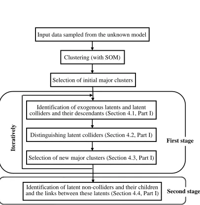
analyzes 2S-PCCs (Definition 18), which are PCCs between major and minor clusters that show two sets (this is the source of “2S” in the name 2S-PCC) of two or more elements in the PCC, and identifies2S-MSOs (Definition 19), which are maximal sets of observed variables that always change their values together in all 2S-PCCs. Different2S-MSOs due to an exogenous latent variable represent latent non-colliders that are descendants of this exogenous variable; hence, LPCC can distinguish between the two types of variables by analyzing2S-MSOs (Theorem 3). To direct the edges between latent non-colliders on a path emerging in an exogenous latent, LPCC checks changes of several 2S-PCCs with re-spect to changes of the latent non-colliders’ exogenous ancestor. Theorem 4 guarantees that LPCC finds all diverging connections and represents all serial connections using a pattern of the true graph, which completes learning the LVM. A flowchart of the LPCC algorithm is given in Figure 1.
A main section of Part II is a formal description of the two-stage LPCC algorithm, which is founded on the PCC concept. Part II also provides an experimental evaluation of LPCC, in comparison to state-of-the-art algorithms, using simulated data sets (Section 3.1) and real-world data sets (Sections 3.2–3.6). The outline of the paper is as follows:
• Section 2: The LPCC algorithmintroduces and formally describes a two-stage algo-rithm that implements the PCC concept;
• Section 3: LPCC evaluationevaluates LPCC, in comparison to state-of-the-art al-gorithms, using simulated data sets (Section 3.1) and real-world data sets (Sections 3.2–3.6);
• Section 4: Related works compares LPCC to state-of-the-art LVM learning algo-rithms;
• Section 5: Discussionsummarizes the theoretical advantages (from Part I) and the practical benefits (from this part) of using LPCC;
• Appendix Aprovides essential assumptions, definitions, propositions, and theorems from Part I;
• Appendix Bsupplies additional results for the experiments with the simulated data sets (Section 3.1); and
• Appendix Cprovides PCC analysis for two example databases.
2. The LPCC algorithm
Asbeh and Lerner
Input data sampled from the unknown model
Clustering (with SOM)
Selection of initial major clusters
Identification of exogenous latents and latent
colliders and their descendants (Section 4.1, Part I)
Distinguishing latent colliders (Section 4.2, Part I)
Selection of new major clusters (Section 4.3, Part I)
Identification of latent non-colliders and their children
and the links between these latents (Section 4.4, Part I)
First stage
Second stage
Ite
rative
ly
2.1 Learning exogenous and latent colliders (LEXC)
LEXC (Algorithm 1) adapts an iterative approach and learns the initial graph in six steps. The first step is clusteringD using the self-organizing map (SOM) (Kohonen, 1997). We chose SOM because it does not require prior knowledge about the expected number of clusters, which is essential when targeting uncertainty in the number of latent variables in the model, but any other clustering algorithm that preserves this property can replace SOM. The result of the first step is a cluster setcin which each clustercis represented by its centroid.
In the second step, LEXC performs an initial selection of the major clusters set (Def-inition 12 in Appendix A), where a cluster incwhose size (measured by the number of clustered patterns) is larger than the average cluster size incis selected as a major cluster (Section 4.3 of Part I).MC={MCi}n
i=1is a matrix that holds information about the major clusters, where each matrix row represents a centroid of one of thenmajor clusters (see, e.g., Table 2 in Part I).
In the third step, LEXC creates a matrix that represents all PCCs (Definition 15), de-rived from MC. This matrix is PCCM={PCCij}n,n
i=1,j>i, where PCCij is a Boolean vector
representing the result of PCC between major clustersciandcj having centroidsMCi and MCj inMC, respectively (see, e.g., Table 4 in Part I). Thek-th element ofPCCij represents
by ”1” a change in value, if one exists, in the observed variableOk ∈Owhen comparing MCi andMCj (for example, Table 4 in Part I shows a change in element 7, corresponding
toX7, ofPCC2,9betweenC2andC9). We use the notationPCCij→δOk if the value ofOk
has been changed andPCCij→ ¬δOkotherwise.
In the fourth step, LEXC identifies exogenous latents and their descendants (Theorem 1) using a matrixMSOSthat holds allMSOs (Definition 16) that always change their cor-responding values together in all major–major PCCs inPCCM. For each identifiedMSOi,
LEXC adds a latentLi toGand to a latent setLand also edges fromLi to each observed
variableO∈MSOi. The observed children of latentLi∈LinGareChi.
In the fifth step, LEXC identifies in two phases, each corresponding to one condition in Theorem 2, the latent variables that are collider nodes in the graph along with their latent ancestors. In the first phase, LEXC considers for each latent variableLi∈L,a set of
potential ancestors from the other latents inL. We call them potential ancestors because another condition should be fulfilled in the second phase to turn them into actual ances-tors. To simplify the notation, we represent the latent as an object and the set of potential ancestors as a field of this object, called PAS (for potential ancestor set). For example, Li.PASrepresents that LEXC identifies a potential ancestor setPASto latent Li. In
addi-tion, we use the notationPCCf g→δLi if all of the variables inChi change their values in PCCf g ∈PCCMand PCCf g → ¬δLi otherwise. In the first phase of the fifth step, LEXC
checks for eachLi ∈Lwhether there exists a vectorPCCf g ∈PCCMin whichLi changes
value together withLj ∈L,but not withLk ∈L,∀k,i, j, and if so, it addsLj toLi.PAS. At
the end of this phase, the setLi.PAScontains all of the latents inLthat change values with
LiinPCCM. Still, this is not enough to decide thatLiis a collider of the variables inLi.PAS.
An additional condition must be fulfilled, which is thatLi should never have changed in
anyPCCf g∈PCCMunless at least one of the variables inLi.PAShas also changed in this
Algorithm 1LEXC
1: Input: Data setDover the observed variablesO
2: Output: GraphGthat includes the exogenous latent variables and the latent colliders and their descendants in LVM
3: Initialize:
4: Create an empty graphGover the observed variablesO 5: c=φ,MC= 0,PCCM= 0,L=φ,MSOS=φ
6: %First step: perform clustering
7: c←perform clustering onDand represent each cluster by its centroid 8: %Second step: select an initial set of major clusters
9: For eachci∈c
10: If the size ofci is larger than the average cluster size inc, then addci toMC. 11: %Third step: create thePCCMmatrix
12: For eachMCi,MCj∈MC,j > i 13: PCCM←computePCCij
14: %Fourth step: identify latent variables and their observed children 15: MSOS←find all possibleMSOs usingPCCM
16: For eachMSOi∈MSOS
17: Add a new latent variableLi toGand toL 18: For each observed variableO∈MSOi 19: AddOand an edgeLi→OtoG
20: %Fifth step: identify latent collider variables and their parents 21: For eachLi∈L
22: % First phase 23: Li.PAS=φ
24: For eachLj∈L,j,i
25: If∃PCCf g∈PCCMs.t (PCCf g →δLi∧ PCCf g→δLj∧PCCf g→ ¬δLk,∀k,i, j), then
26: AddLj toLi.PAS 27: % Second phase
28: if∀PCCf g∈PCCMs.tPCCf g →δLi 29: ∃P AS∈Li.PASs.tPCCf g→δP AS
30: then∀P AS∈Li.PAS, add a new edgeP AS→LitoG. 31: %Sixth step: search for a new set of major clusters 32: NMC=φ
33: Find the cardinality of eachLi∈L, then identifyexs 34: For eachex∈exs
35: Findc∗=argmaxc∈cP(c|ex) and addc ∗
toNMC 36: IfNMC=MC
37: ReturnG 38: Else
if fulfilled, it adds an edge from each variable inLi.PAStoLito complete the identification
ofLias a collider.
In the sixth and last step, and to deal with possible false positive and false negative errors (Section 4.3 of Part I), LEXC searches for a new set of major clustersNMC based on the already learned graph and all the clusters that initially were identified by SOM. First, LEXC learns for each latent Li ∈Lits cardinality, which is the number of different
value configurations of Li corresponding to all value configurations of Chi in D. Each such value configuration of observed children is due to a value li of Li, and we denote
it by li →chi. Then, LEXC finds the set of all possible exs (all possible configurations
of all exogenous latents in L, Li ∈ L∩EX). For each ex, LEXC finds the most probable
cluster, c∗ = argmaxc∈cP(c|ex), where the posterior probability P(c|ex) for each c ∈ c is
approximated by the ratio betweenc’s size and the size of D. Thus, the cluster for which the values corresponding to the children ofLi∈L∩EX,li→ch
i, are most probable due to
li inexis selected as the most probable to represent this ex. Each such cluster is added
toNMC. IfNMC=MC,NMCcannot improve the graph, and thus LEXC stops and returns the learned graph G. Otherwise, LEXC reinitializes MC to be NMCand relearns a new graph.
2.2 Learning latent non-colliders (LNC)
Using the data setD, LNC has to split the set of latent variablesLin graphG, which was learned by LEXC, into exogenous latents and latent non-colliders. First, LNC (Algorithm 2) adds |L| elements to the end of each vector in D and creates an incomplete data set
IND. For a vector inINDfor which values of the observed children for a specific latent Li ∈ L take major values, the value of the latent can be reconstructed exactly, li →chi;
however, when not all observed children take major values, this value of the latent cannot be reconstructed, and this is the reason why IND is incomplete. Second, using the EM algorithm (Lauritzen, 1995; Dempster et al., 1977) andIND, LNC learns (Section 4.4 of Part I)G’s parameters and uses them to compute a threshold (Appendix B in Part I) on the maximal size of 2-MCs. This threshold is needed to find 1-order minor clusters (1-MCs; Definition 14). Note that after learning the parameters, the graph turns into a model, M0. Third, for each exogenous latent EXi ∈ L∩EX in turn, LNC tests ifEXi should be split
(Section 4.4 of Part I). For this test, LNC needs first to find the set of 1-MCs forEXi and
compute all the PCCs between these clusters and the major clusters forEXi. We denote
the set of these PCCs byPCCS. Then, LNC finds all the PCCs inPCCSthat are2S-PCC
(Definition 18); these will be used to identify all possible2S-MSOs (Definition 19) and thus all possible latent non-collider descendants that should be split fromEXi (Theorem
3).
After identifying the latent non-colliders’ descendants ofEXiand splitting them from
EXi, LNC finds the links between these latents (Section 4.4 of Part I). LNC first finds the
setL’of all latents whose children change alone in some 2S-PCCs. These are the candidates to beEXi or its leaves (Proposition 10). Then, for eachL’∈L
0
, LNC finds the 2S-PCCs in
between them using Theorem 4. Note that, we assume by default thatL’is a leaf, so LNC does not need to redirect the links in the diverging connection case. After finding all the possible directed paths, LNC identifies if the connection is serial (in case|L’|is exactly two)
and if so it makes the links on this path undirected; otherwise, the path is directed as part of a diverging connection. Finally, LNC returns a patternG, which represents a Markov equivalence class of the true graph.
Algorithm 2LNC
1: Input: Data setDover the observed variablesOand the graphGlearned by LEXC 2: Output: The final learned LVMG
3: Initialize:IND =0, PCCS=φ,2S-PCC=φ,2S-MSOS=φ,2S-PCC’=φ 4: CreateIND(see text)
5: LearnG’s parameters using the EM algorithm to obtain an LVM, M0 6: For each latentEXi∈L
7: % Identify and split the latent non-collider descendants ofEXi 8: Find the set of 1-MCs according to M0
9: PCCS←compute all PCCs between the 1-MCs and the major clusters forEXi 10: 2S-PCC←find all 2S-PCCs inPCCS
11: 2S-MSOS←find all possible2S-MSOs using2S-PCC 12: For each2S-MSOj∈2S-MSOS
13: Add a latent non-colliderN CjtoEXi,L,andG 14: For each observed variableO∈2S-MSOj
15: SplitOfrom the children ofEXiand add an edgeN Cj→OtoG
16: % Identify the links between the new latent non-colliders that were split fromEXi
17: L’←all latents that were split (includingEXi) and whose observed children change alone in some 2S-PCC
18: For eachL’∈L0% assume by defaultL’is a leaf and apply Theorem 4
19: 2S-PCC’←all 2S-PCCs in2S-PCCin which the observed children ofL’ do not change 20: For each two latent non-collidersN Cj, N Ck,k,jthat were split fromEXi:
21: If
22: 1) the observed children ofN Ckalways change with those ofN Cj in2S-PCC’; and 23: 2) the observed children ofN Cjchangettimes and the observed children ofN Ck
changet+1times in2S-PCC’
24: Then add a directed edge fromN CktoN CjtoG
25: % Identify if the connection is serial, and if so make the links in the path undirected 26: If|L0|=2
27: If there are two paths with the same latents but opposite directions, then make the edges between the latents undirected.
28: ReturnG
3. LPCC Evaluation
a mass cytometry data set of the immune system (Section 3.6). In the case of the real-world data sets, we did not have an objective measure for evaluation; thus, we compared the LPCC output to hypothesized, theoretical models from the literature and to the out-puts of four state-of-the-art learning algorithms. The first algorithm is FCI (Spirtes et al., 2000), and because we noticed (see below) for the political action survey and Holzinger and Swineford’s data sets that FCI is not suitable for learning MIM models, we did not use it for the other data sets. The second algorithm is for learning HLC models (Zhang, 2004), and since the theoretical models for all but the HIV data set are not latent-tree mod-els, we used this algorithm only for the HIV data set. The third algorithm is exploratory factor analysis (EFA). Because the theoretical models for the political action survey and Holzinger and Swineford’s data set were already tested by confirmatory factor analysis [(Joreskog, 2004); (Arbuckle, 1997, p. 375); and (Joreskog and Sorbom, 1989, p. 247)], we completed the examination of EFA also to the YD and mass cytometry data sets. The fourth algorithm, which is actually two algorithms, BuildPureClusters (BPC) and BuildS-inglePureClusters (BSPC) of Silva (2005), is especially suitable for MIM models. BPC is Silva’s (2005) main algorithm; hence, we used it in all the evaluations. BPC assumes that the observed variables are continuous and normally distributed, whereas BSPC is a variant of BPC for discrete observed variables. We ran BPC using its implementation in the Tetrad IV package, which can take discrete data (as in all the data sets in this evaluation) as input and treat them as continuous.4 BPC learns LVM by testing Tetrad constraints at a given significance level (alpha). We used Wishart’s Tetrad test (Silva, 2005; Spirtes et al., 2000; Wishart, 1928), applying three significance levels of 0.01, 0.05 (Tetrad’s default), and 0.1. For the simulated data sets, we compared LPCC to EFA and BPC.
3.1 Evaluation using simulated data sets
We used Tetrad IV to construct the graphs G1, G2, G3, and G4 of Figure 2, once with binary and once with ternary variables. The priors on the exogenous latents were al-ways distributed uniformly. We compared performances for three parameterization lev-els that differ by the conditional probabilities, pj=0.7, 0.75, and 0.8, between a latent
Lk and each of its children ENi. For all graphs in the binary case, except L2 in G2,
P(ENi=v|Lk=v) = pj, v = 0 or 1. For all graphs in the ternary case, except L2 in
G2, P(ENi=v|Lk=v) = pj, P(ENi,v|Lk=v) = (1−pj)/2, v = 0, 1, or 2. Concerning
L2 in G2, P(L2= 0|L1L3= 00,01,10) = P(L2= 1|L1L3= 11) =pj in the binary case and
P(L2=v|max{L1, L3}=v) = pj and P(L2,v|max{L1, L3}=v) = (1−pj)/2 in the ternary
case. Each such scheme imposes a different “parametric complexity” on the model and thereby affects the task of learning the latent model and the causal relations. That is, usingpj=0.7 poses a larger challenge to learning thanpj=0.75, which poses a larger
chal-lenge thanpj=0.8. For example for G3 and the binary case, the correlations between any
latent and any of its children for the parametric settingspj=0.7, 0.75, and 0.8 are 0.4, 0.5,
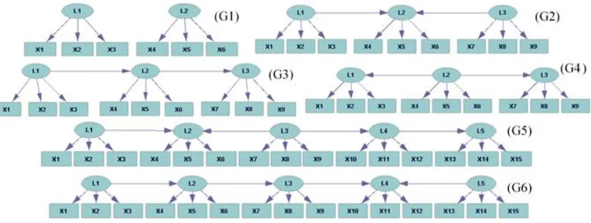
Figure 2: Example LVMs that are all MIMs. Each is based on a pure measurement model and a structural model of different complexity, posing a different challenge to a learning algorithm.
and 0.6, respectively. Note that correlation of 0.4 is relatively low, providing a great chal-lenge to the learning algorithms, and trying to learn an LVM for lower correlation values yields poor results by all algorithms.5 Tetrad IV was also used to draw data sets of 125, 250, 500, 750, 1000, and 2,000 samples for each test. Overall, we evaluated the LPCC algorithm using 144 synthetic data sets for four graphs (G1–G4), two types of variables, three parameterization levels, and six data set sizes.
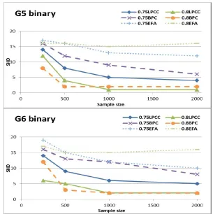
In addition, we evaluated LPCC using the two large graphs in Figure 2, G5 and G6, which combine all types of links between the latents, such as serial, converging, and di-verging. Each graph has five latents with three observed children each. Tetrad IV was used to draw data sets of 250, 500, 1000, and 2,000 samples, where all variables are binary and for two parametric settingspj=0.75 and 0.8. In all cases, we report on the structural
hamming distance (SHD) (Tsamardinos et al., 2006) as a performance measure for learning the LVM structure. SHD is a global structural measure that accounts for all the possible learning errors: addition and deletion of an undirected edge, and addition, removal, and reversal of edge orientation.
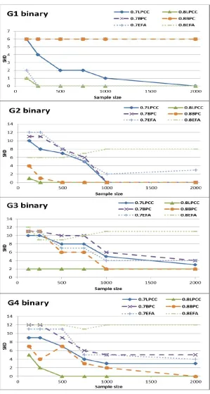
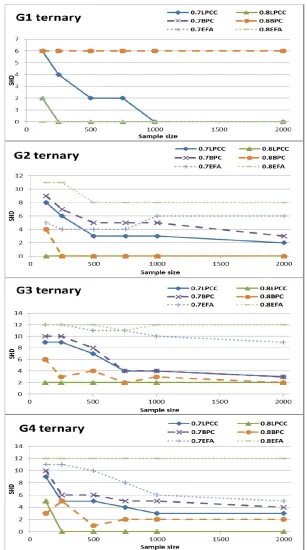
Figures 3–5 show learning curves for SHD (the lower value is the better one) and in-creasing sample sizes for LPCC, BPC, and EFA. Figures 3 and 4 show SHD performance in learning G1–G4 with binary variables and ternary variables, respectively, and for two parametric settings,pj=0.7 and 0.8. Figure 5 shows performance in learning G5 and G6
with binary variables for two parametric settings pj=0.75 and 0.8 (for pj=0.7 the
algo-rithms performed poorly and thus their results are excluded here). In addition, in Ap-pendix B, we compare LPCC with BPC (Section B.1) and with EFA (Section B.2) in learn-ing G1–G4 with binary and ternary variables for three parametric settlearn-ings, pj=0.7, 0.75,
and 0.8. The graphs demonstrate the LPCC sensitivity to the parametric complexity – the
Figure 5: SHD learning curves of LPCC compared to those of BPC and EFA for G5 and G6 of Figure 2 with binary variables, two parameterization levels, and increasing sample sizes.
lower the complexity is, the faster learning is and the sooner the error vanishes – and the LPCC good asymptotic behavior, demonstrating accuracy improvement with the sample size. Generally, Figures 3–5 (and those in Appendix B) show superiority of LPCC over BPC and EFA; LPCC demonstrates higher accuracies (smaller errors) and a better asymptotic behavior than BPC and EFA.
and all graphs but G1. Independent latent variables, as manifested in G1, is the ultimate prerequisite for a successful application of EFA, and indeed, EFA shows competitive (and sometimes, for small sample sizes, even slightly improved) performance to LPCC in learn-ing G1.
Unlike LPCC, BPC is not suitable for learning models such as G1, where the latents are independent and each has fewer than four observed children. This is because BPC requires the variables in a Tetrad constraint to all be mutually dependent, where in the case of G1, there are at most three mutually dependent variables, so no Tetrad constraint can be tested, and no graph is learned (SHD=6 for missing all the six edges in G1). However, it is reasonable to assume that a practitioner would naturally analyze the data before trying BPC, and if they recognize that not all observed variables are correlated (e.g., X1 and X4 for G1), then they will not use BPC. As Figures 3–5, together with the more detailed Figures 17 and 18 in Appendix B, demonstrate, for most graphs, parametrization levels, and sample sizes (except for some cases with small sample sizes), LPCC is superior to BPC.
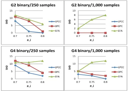
Another view of these results is manifested in Figure 6 that shows SHD values for the LPCC, BPC, and EFA algorithms for increasing parametrization levels for four com-binations of learned graphs and sample sizes. Figure 6 shows that both LPCC and BPC improve performance, as expected, with increased levels of latent-observed variable cor-relation (pj). LPCC never falls behind BPC, and its advantage over BPC is especially vivid
for a small sample size. EFA, besides falling behind LPCC and BPC, also demonstrates worsening of performance with increasing the parametrization level, especially for large sample sizes, for the reasons provided above.
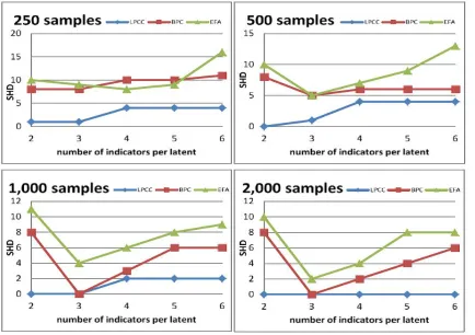
Finally, we expand the evaluation by examining the algorithms when the number of indicators a latent has increases. Figure 7 shows the SHD values of the LPCC, BPC, and EFA algorithms for increasing numbers of binary indicators per latent variable in G2, a parametrization level (pj) of 0.75, and four sample sizes. The figure exhibits clear
supe-riority of LPCC over BPC and EFA for almost all numbers of indicators and sample sizes. While LPCC hardly worsens its performance with the increase of complexity (number of indicators a latent has), both BPC and EFA are affected by this increase. Also worth men-tioning is the difficulty these two latter algorithms have in learning an LVM for which latent variables have exactly two indicators, regardless of the sample size.
To understand the differences among the three algorithms in more detail, we analyze the errors they make, for example, when using 1,000 samples (the reference is the bottom-left graph in Figure 7). When the number of indicators a latent has is less than 4, LPCC learns the LVM perfectly, and when this number is greater, LPCC errs twice in missing an edge from a latent to one of its indicators. BPC cannot learn an LVM using two indica-tors per latent, and thus it misses all eight edges in G2 and returns an empty graph. It successfully learns the LVM when each latent has exactly three indicators, but then fails to direct the edges among the latent variables and misses at least a single edge between a latent and an indicator when the latent variables have more than three indicators each. For two indicators per latent, EFA detects only two factors and fails to connect them. It connects one factor to six indicators and the second factor to five indicators, and thereby errs in learning seven extra edges from latent variables to observed variables, missing two edges from the missing latent variable to two observed variables, and missing the two edges among the latent variables, which accounts for eleven errors in total. For three in-dicators per latent, EFA detects three inin-dicators for two of the latents and five inin-dicators for the other and misses the edges among the latents, which accounts for four errors in total. For four to six indicators per latent, EFA learns more extra edges between the latent and observed variables, together with missing the edges among the latents. This exper-iment vividly demonstrates the advantage of LPCC over BPC and EFA in that not only does LPCC detect edges between latent and observed variables more accurately, but it also detects latent-latent connections in all scenarios, which is impressive especially when the sample size is small and/or the number of indicators a latent has is large.
3.2 The political action survey data
We evaluated LPCC using a simplified political action survey data set over the following six variables (Joreskog, 2004):
• NOSAY: “People like me have no say in what the government does.”
• VOTING: “Voting is the only way that people like me can have any say about how the government runs things.”
• COMPLEX: “Sometimes politics and government seem so complicated that a person like me cannot really understand what is going on.”
• NOCARE: “I don’t think that public officials care much about what people like me think.”
• TOUCH: “Generally speaking, those we elect to Congress in Washington lose touch with people pretty quickly.”
• INTEREST: “Parties are only interested in people’s votes, but not in their opinions.”
sample of 1,076 United States respondents. A model consisting of two latents that corre-spond to a previously established theoretical trait of Efficacy and Responsiveness based on Joreskog (2004) is given in Figure 8a. VOTING is discarded by Joreskog for this particular data based on the argument that the question for VOTING is not clearly phrased.
Similar to the theoretical model, LPCC finds two latents (Figure 8b): One corresponds to NOSAY and VOTING and the other corresponds to NOCARE, TOUCH, and INTEREST (a detailed description of the PCC analysis that led to these results is in Appendix C). Compared with the theoretical model, LPCC misses the edge between Efficacy and NO-CARE and the bidirectional edge between the latents. Both edges are not supposed to be discovered by LPCC or BSPC/BPC; the former because the algorithms learn a pure mea-surement model in which each observed variable has only one latent parent and the latter because no cycles are assumed. Nevertheless, compared with the theoretical model, LPCC makes no use of prior knowledge.
Figure 8: The political action survey: (a) A theoretical model (Joreskog, 2004) and five outputs of (b) LPCC, (c) BSPC, (d) BPC for alpha=0.01 and 0.05, and (e) BPC for alpha=0.1.
identify VOTING as a child of Efficacy (at the expense of COMPLEX), and thereby chal-lenge the decision made in Joreskog (2004) to discard VOTING from the model. The out-puts of the BPC algorithm (Figure 8d) for both alpha=0.01 and alpha=0.05 are poorer than those of LPCC and BSPC. BPC finds two latents. The first latent corresponds to NOSAY, VOTING, and COMPLEX with partial resemblance to the theoretical model (identifying NOSAY and COMPLEX as indicators of this latent) and partial resemblance to the outputs of LPCC and BPC (identifying NOSAY and VOTING as indicators of the latent). However, the second latent found by BPC corresponds only to TOUCH and misses INTEREST (iden-tified in the theoretical model and by LPCC and BSPC as an indicator of Responsiveness) and NOCARE (that is identified in the theoretical model and by LPCC as an indicator of Responsiveness). The output of the BPC algorithm using alpha=0.1 (Figure 8e) gives very little information about the problem as it finds only one latent that corresponds only to NOCARE. These last two figures show the sensitivity of BPC to the significance level, which is a parameter whose value should be determined beforehand. Note that the suc-cess of the LPCC and BSPC algorithms emphasizes the importance of such algorithms in learning discrete problems.
The outputs of the FCI algorithm using any of the above significance levels are not sufficient (Figure 9). For example, the FCI outputs that were learned using alpha=0.01 (Figure 9a) and 0.05 (Figure 9b) show that NOSAY and INTEREST potentially have a la-tent common cause. However, these two variables are indicators of different latents in the theoretical model. These results are understandable because unlike LPCC, BPC, and BSPC, FCI is not suitable for learning MIM models such as the political action survey.
3.3 Holzinger and Swineford’s data
Holzinger and Swineford (1939) collected data from 26 psychological tests administered to 145 seventh- and eighth-grade children in the Grant-White School in Chicago, Illinois. In this evaluation, we use a subset of this data over only six variables representing the scores in six intelligence tests. The variables are: scores on a visual perception test (Vis-Perc), scores on a cube test (Cubes), scores on a lozenge test (Lozenges), scores on a para-graph comprehension test (ParComp), scores on a sentence completion test (SenComp), and scores on a word meaning test (WordMean). There are two hypothesized intelligence factors, which are spatial ability and verbal ability factors. The first three variables mea-sure spatial ability and the latter three variables meamea-sure verbal ability. A confirmatory factor model that fits this data well was extracted from the Amos manual (Arbuckle 1997, p. 375; Joreskog and Sorbom 1989, p. 247) and is shown in Figure 10a.
We ran LPCC using a dichotomous (binary) presentation of the continuous data. For each variable, scores that were above the average score were recoded as 2, and scores be-low the average score were recoded as 1. Despite the small size of the data set and the loss of information due to the discretization process, LPCC found two latents (Figure 10b). The first latent corresponds to VisPerc and Lozenges, and the other latent corresponds to ParComp, SenComp, and WordMean (a detailed description of the PCC analysis is in Ap-pendix C). Our model matches the theoretical model, except for missing one link between Spatial and Cubes (and the link between the latents that the model is not supposed to identify).
The outputs of the BPC algorithm using alpha=0.01 and 0.05 (Figure 10c) were not good compared to the theoretical model and LPCC output. In both cases, BPC found only a single latent variable that corresponds to only four of the six indicators, specifically, VisPerc, Lozenges, Cubes, and WordMean. Notice that WordMean and the other three variables belong to two different latent variables in the theoretical model. However, for a significance level of 0.1, BPC output (Figure 10d) is the closest of all models to the the-oretical model. These results show the sensitivity of BPC to the significance level, which is a parameter that does not have a predetermined value. LPCC does not have this dis-advantage. Note that the superiority of BPC for a significance level of 0.1 for Holzinger and Swineford’s data set is in contrast to the model inferiority for other significance levels (Figure 10c) and for the political action survey data set with any significance level.
Figure 10: (a) A theoretical model for Holzinger and Swineford’s data set based on a con-firmatory factor model that fits this data well and the outputs of (b) LPCC, (c) BPC for alpha=0.01 and 0.05, and (d) BPC for alpha=0.1.
have a latent common cause, and Lozenges, VisPerc, and Cubes potentially have another latent common cause. This model matches the theoretical model (Figure 11a) except for the bidirectional edge between the latents.
3.4 The HIV test data
Figure 11: FCI outputs for Holzinger and Swineford’s data set and significance levels of (a) 0.01 and 0.05, and (b) 0.1.
Figure 12: Model learned for HIV using LPCC.
3.5 Explanation of young drivers’ involvement in road accidents using LPCC
of traffic offenses for the first six months after obtaining a driving license. YDs in the two databases were grouped according to the following classes:
DB1:
Accident and offense: All YDs who had at least one accident and committed at least one offense in the three-month period after ADP (the “period”). There were 345 such drivers; hence, this number defined a group size.
Offense but no accident: 345 drivers who committed at least one offense, but had no acci-dents in the period.
Accident but no offense: 345 drivers who had at least one accident, but committed no of-fense in the period.
No accident and no offence: 345 drivers who did not have any accidents or commit any offenses in the period.
In total, there are 1,380 observations (YDs) for DB1.
DB2:
Accident and offense: All YDs who had at least one accident and committed at least one offense in the period (similar to this class in DB1).
No accident and no offense: 345 drivers who did not have any accidents or commit any offenses in the period (similar to this class in DB1).
In total, there are 690 observations (YDs) for DB2.
All observations in both databases are represented by thirteen observed variables that a previous study indicated as relevant to the explanation of YD involvement in road ac-cidents and offenses (Lerner, 2012; Lerner and Meyer, 2012). In addition, we used four observed variables that indicate if YDs or their parents were involved in a road accident or an offense. A detailed description of all seventeen observed variables is given in Table 1.
0.7 level corresponds to about half of the variance in the indicator being explained by the factor. However, the 0.7 standard is high, and real-world data may not meet this criterion, which is why some researchers, including us in this study (particularly for exploratory purposes such as this case), use a lower level, where 0.4 is the common practice (Manly, 1994). In addition, we adapted Occam’s razor parsimony principle (to explain the variance with the fewest possible factors) and required the variance explained criterion to be above 50%.
Number Variable Variable short name
Variable values
1 Age gil 1 (17–18), 2 (19–20), 3
(21–22), 4 (23–24)
2 Gender Min 1 (male), 2 (female)
3 Medical limita-tions
lim 1 (no), 2 (yes)
4 Father is
al-lowed to drive
MurF 1 (yes), 2 (no)
5 Mother is
al-lowed to drive
MurM 1 (yes), 2 (no)
6 Has a
motorcy-cle license
of 1 (no), 2 (yes)
7 Received “Or
Yarok” kit, as part of a grad-uated driver licensing pro-gram6
or 1 (didn’t receive), 2 (re-ceived)
8 Socioeconomic index
GF 1–4 (1–low, 4–high)
9 Ethnic group KU 1 (Jew), 2 (non-Jew)
10 Father’s marital status
FS 1 (single), 2 (married), 3 (divorced), 4 (widowed) 11 Mother’s
mari-tal status
MS 1 (single), 2 (married), 3 (divorced), 4 (widowed) 12 Father’s number
of years of edu-cation
FED 1–4 (1–low, 4–high)
13 Mother’s
num-ber of years of education
MED 1–4 (1–low, 4–high)
14 Offenses of YD OFYD 1 (no), 2 (yes) 15 Accidents of YD ACYD 1 (no), 2 (yes) 16 Offenses of
par-ents
OFPA 1 (no), 2 (yes)
17 Accidents of
parents
ACPA 1 (no), 2 (yes)
Results for DB1:
Figure 13: LVMs learned by EFA, LPCC, and BPC for DB1. Numbers for EFA represent the factor loadings, where plus and minus signs indicate positive and negative correlation, respectively.
Both LPCC and EFA found six latent variables (Figure 13). L1 in EFA is a parent of five observed variables, where each describes another aspect of the demographic or socioeco-nomic state of the YD or his/her family. The variables (see Table 1)father is allowed to drive (MurF),mother is allowed to drive(MurM), age (gil), and ethnic group (KU) are positively associated, whereas the variablesocioeconomic index(GF) is negatively associated with L1. Based on the values of these variables, we can identify groups in the YDs’ population, such as a group of YDs that are not Jewish, their parents are not allowed to drive, and their age and their socioeconomic status are low. L1 is not connected by EFA to other la-tent variables that relate to YD involvement in road accidents or offenses; thus, it does not contribute much to this study. However, L1 and L2 as learned by LPCC relate the socioe-conomic state of the YD family (GF and KU are children of L1) with YD offenses (OFYD
is a child of L2), thus LPCC links the socioeconomic state of YD with its involvement in traffic offenses. For example, according to LPCC, a YD who is not Jewish, with a low so-cioeconomic index, and whose mother is not allowed to drive is more likely to be involved in traffic offenses.
Latents L2 in EFA and L3 in LPCC describe the educational status of the YDs’ parents and indicate a similar tendency between the parents’ educational levels. However, both EFA and LPCC analyses do not link the educational status of the YD family to involvement in road accidents and traffic offenses.
L3 in EFA shows a negative relationship between a YD’s gender (Min) or having a motorcycle license (of) and his/her tendency to commit road offenses. Male drivers tend to commit more traffic offenses than female drivers, and drivers who have a motorcycle license tend to commit more traffic offenses than drivers who do not have such a license. L4 in EFA shows the marital status of the YD parents, and not surprisingly, it indicates that the father’s and mother’s marital status is correlated. L5 in EFA shows that the parents of YDs who did not receive the “Or Yarok kit” tend to commit more traffic offenses. That is, the introduction of the kit in the family seems to also reduce involvement in road offenses of family members other than the YD. L6 in EFA shows a negative relationship between YD involvement in road accidents and the involvement of their parents in accidents. One explanation for this negative relationship could be that in a family in which one member was involved in an accident, other members tend to be more careful and thus decrease their involvement in accidents. Due to the independency assumption (between the factors) in EFA, L3, L4, L5, and L6 are not related, and EFA is not able to holistically represent relations among variables representing demographic and socioeconomic characteristics and road accidents and offenses of YDs and their parents.
LPCC describes involvements in road accidents and offenses in a more comprehensive way using a structure that is based on three latents with a diverging link from L5 to L4 and L6. L5 shows a relationship among the variablesmotorcycle license,received “Or Yarok kit”, mother’s marital status, and parents’ involvement in accidents. For example, it was found that there is a relation between receiving the “Or Yarok kit” and decreasing values of par-ents’ involvement in accidents. However, we note that the variable parpar-ents’ involvement in accidents is sparse in DB1, making its relationship with the other variables via L5 quite arguable. An interesting relationship found in the LPCC results is between parents’ ac-cidents (child of L5) and parents’ offenses (child of L6). This relationship was missed by EFA since each variable in EFA is a child of a different latent that is independent of the other latent (due to EFA’s orthogonality assumption).
of their parents (OFPA), a relation that seems reasonable and is not identified by EFA and LPCC. However, the identification of OFYD as L1’s child and OFPA as L2’s child implies that it is the YD offenses that affect the offenses of their parents and not the opposite, as may be expected. Another relation that is identified only by BPC is between the mother’s education level (MED) and both YDs’ and their parents’ offenses.
Results for DB2:
Figure 14: LVMs learned by EFA, LPCC, and BPC for DB2. Numbers for EFA represent the factor loadings, where plus and minus signs indicate positive and negative correlations, respectively.
between YDs’accidentsandoffensesvariables is due to the linkage formed in the database by creating it from observations of YDs having both accidents and offenses or neither. Yet, both EFA and LPCC did not manage to find a relation between YDs’ accidents and offenses and their parents’ accidents and offenses.
L2 in EFA describes the socioeconomic status of the YD family, similar to L1 in the EFA results for DB1 (but without thefather is allowed to drivevariable). Again, it shows groups in the YD population, such as a group of YDs who are not Jews, whose mothers are not allowed to drive, and whoseageandsocioeconomicstatus are low.
L2 and L3 in LPCC also represent the social status of the YD family. L2 explains the family educational level (as L3 in LPCC for DB1), and L3 is a demographic latent that is a parent of the ethnic group and the mother is allowed to drivevariables. Unlike L2 in EFA, which also represents economic status via the variablesocioeconomic index(GF), L3 in LPCC is only a social variable. Furthermore, L3 in LPCC did not link the age variable to the social representation of YD (as L2 did in EFA). It is also interesting to see the relation that LPCC found between latents L2 and L3, which is between the parents’ education levels (L2) and the family demographic status (L3). But, LPCC did not find a relation between L2 and L3 and theaccidentsandoffensesvariables of the YDs or their parents.
L4 in EFA shows the marital status of the YD’s parents, similar to the EFA results for DB1. L5 in EFA shows that parents of a YD who did not receive the “Or Yarok kit” tend to commit more road offenses, again similar to the EFA results for DB1. L6 shows a relation between the YD’s medical limitations and his/her parents’ involvement in accidents; this relation is hard to intuitively explain. Similar to DB1, there are no relations between the latents L4–L6 due to the independency assumption of EFA; hence, there is no relation between the latent that represents the parents’ marital status and their involvement in accidents or offenses.
and its children. The information about the relationships between the latents that LPCC provides illustrates the added value of using such an algorithm in causal analysis.
Also for DB2, it seems that BPC yields poorer results than LPCC. L2 in BPC is partially equivalent to L1 in LPCC (without OFYD), and some resemblance can be seen between L3–L4 in BPC and L4–L6 in LPCC. L2 and L3 in BPC are parents of L4, which together link medical limitations of the YD and whether the mother is allowed to drive with ACYD and OFPA (although we would expect the former two to be causes of the latter two and not the opposite). However, each of the two remaining latents in the BPC model has only a single observed variable as a child, which gives very little information about the problem. L5 in BPC has a single child, MED, without linking it to FED, although these two variables are highly correlated, as in both the EFA and LPCC models. The same can be said about L1 and its child MS that is not linked to FS, although both are correlated. These two are directly connected in the EFA model and indirectly connected in the LPCC model.
3.6 Identification of cellular subpopulations of the immune system from mass cytometry data sets using LPCC
Definition of immune cell subsets is usually based on flow cytometry data. However, this approach suffers from severe limitations in the number of cellular markers that can be measured simultaneously. Currently, flow cytometry permits the concurrent measurement of only 12–17 cellular markers. A recent technological development in single cell measure-ment is mass cytometry or cytometry by time of flight (CyTOF). This method allows for quantification of hundreds of thousands of single cells at high dimension (currently up to 40 cellular markers can be measured) in a sample. CyTOF yields phenotypically rich datasets that enable a more accurate identification of cellular subpopulations. Clustering and visualization methodologies have been developed to identify meaningful cell subsets in CyTOF data. However, none provide a systematic and automatic method for identifying the cellular subpopulations represented by these clusters.
We evaluated LPCC’s ability to automatically identify such cellular subpopulations in an unsupervised manner and in comparison to BPC and EFA (using the same settings as in Section 3.5). We used a CyTOF-generated dataset of mouse splenocyte samples, collected from 20 mice and stained with a panel containing 37 metal-labelled antibodies. We ran-domly selected 40,000 single cell measurements from each sample to have 800,000 obser-vations. Cellular markers measured by CyTOF have continuous multimodal distributions. Since LPCC works on discrete observed variables, we needed to perform discretization first. To this end, we randomly selected 40,000 observations for each cellular marker and used this sample to learn a mixture of Gaussians, approximating each marker’s distribu-tion [with the number of components selected from K=3-10 using the Bayesian Informa-tion Criterion (BIC)]. Next, the learned Gaussian components were sorted by their means, and the ordered means determined the K discrete values of the marker. Thus, K also rep-resents the cardinality of the marker after the discretization. Finally, for each marker, each observation in the data set was assigned the closest discrete value.
mark-ers between these cellular subpopulations. This observation is demonstrated clearly in the results obtained by BPC, EFA, and LPCC in Figures 15a, 15b, and 16a, respectively. LPCC and EFA managed to learn models with eight latents each and BPC a model with one la-tent, but none of the three latent variable models seems to be biologically meaningful, as judged by biological experts.
However, LPCC has an advantage over the other two algorithms because to advance learning an LVM, LPCC clusters the input data in its first stage. We exploit this advantage by improving clustering of the input to consider the domain specific properties. This act of clustering – that is natural to LPCC – coincides with the conventional clustering-based analysis of CyTOF data, which is mandatory to this domain because the data shows a hierarchical structure (as outlined below). Therefore, instead of using SOM, we initialized LPCC based on the clustering results obtained by Citrus (Bruggner et al., 2014). Citrus applies hierarchical clustering to the cell events; however, instead of cutting the hierarchy at an arbitrary height to identify the clusters, it uses a minimum cluster size threshold (we used a 1% threshold of the observations, i.e., 8,000 observations), for which only clusters larger than this threshold are selected. By selecting automatically and based on the data only large enough clusters, we preserve the requirement of LPCC of not determining the number of clusters arbitrarily and facilitate the avoidance of noisy clusters. In addition, we performed another purification procedure by selecting only clusters for which the ratio of the cluster marker entropy to the distribution marker entropy is smaller than a threshold. Following this cluster purification procedure, LPCC found a five-latent variable model that is represented in Figure 16b. L1 is a parent of five markers that represent T cells (except for CD457 that may be expressed also by other leukocytes, and CD62L that is an activation marker that also can be expressed by T cells). L2 partially represents monocytes by having the markers CD11b and CD86 as its children; however, this representation is not perfect since it wrongly connects CD34, which is a phenotypic marker of stem cells. Thus, L2 may be representing monocytes that are antigen-representing cells excluding CD34. L3 and L4 are linked by a directed edge from L3 into L4 and together represent macrophage cells. Although both latents represent the same population of cells, LPCC correctly splits it into two latent variables since the children of L3 are expressed only by macrophages, but the children of L4 may also be expressed by monocytes, which are the macrophages’ precursor. L5 is a parent of three markers that represent B cells together with another marker, IA-IE, which is an activation marker that can also be expressed by B cells. Still, the model learned by LPCC represents only sixteen of the 37 markers in this experiment. This may be explained by the high level of overlap and number of shared markers among the different subpopulations. Despite that, these results are encouraging and demonstrate a significant improvement compared to previous results obtained by BPC, EFA, and LPCC before cluster purification.
Analysis of cell sub-populations in the immune system naturally lends itself to the use of clustering methodologies, as immunologists traditionally resort to the classification of cells as belonging to cellular subpopulations. Cell subpopulations are usually defined by the stable expression of markers on said cells. Yet, not all markers capture protein expres-sion that is stably expressed, and the expresexpres-sion of some proteins may be noisy or plastic,
varying over time and conditions. With this in mind, clustering and noise filtration – two pre-processing steps of LPCC – provide great benefit in this context, yielding improved results. Specifically, the pre-processing step of clustering the data prior to LPCC provides an advantage as it compartmentalizes marker relationships to the context in which they matter, whereas the noise filtering step focuses the analysis to those markers whose rela-tionship with one another may be meaningful.
4. Related Works
The traditional framework for discovering latent variables is factor analysis and its vari-ants (e.g., see Bartholomew et al., 2002). This is, by far, the most common method used in several applied sciences (Glymour, 2002). However, a limitation of factor analysis is its level of subjectivity stemming from the many methodological decisions a researcher must make to complete an analysis, where the results of this analysis largely depend on the quality of these decisions (Henson and Roberts, 2006). Moreover, factor analysis and its variants provide only a limited ability in causal explanation (see Silva, 2005, and our eval-uation section). Therefore, in this section, we will focus on related work in the framework of learning causal graphical models beyond the variants of factor analysis.
The main goal of heuristic methods such as those of Elidan et al. (2000) is the reduction of the number of parameters in a BN. The idea is to reduce the variance of the resulting density estimator, achieving better probabilistic predictions. For probabilistic modeling, the results described by Elidan et al. are a convincing demonstration of the suitability of their approach, which is intuitively sound. However, such heuristic methods provide nei-ther formal interpretation of what the resulting structure is, nor explicit assumptions on how such latents should interact with the observed variables. Further, such heuristic meth-ods do not provide an analysis of possible equivalence classes, and consequently, there is no search algorithm that can account for equivalence classes. Therefore, for a causality discovery under the assumption that multiple observed variables have hidden common causes, such as in MIM that is widely used in applied sciences, the results described by Elidan et al. are unsatisfying.
Unlike other algorithms (Pearl, 2000; Zhang, 2004; Harmeling and Williams, 2011; Wang et al., 2008), LPCC is suitable for learning MIM models and not just latent-tree models. This LPCC quality is shared by BPC (Silva et al., 2006). Both LPCC and BIN-A (Harmeling and Williams, 2011) apply clustering as a preprocessing step to learn latent models. But, LPCC applies clustering to the data points, whereas BIN-A clusters the vari-ables using agglomerative hierarchical clustering, which is suitable to learn HLC models, as in Zhang (2004). LPCC provides a consistent and substantive analysis of data-point clustering using the PCC concept and can learn all types of links between the latents; thus, unlike BIN-A, it is not limited to binary latent trees.
FCI (Spirtes et al., 2000) is not comparable to LPCC in learning MIM models as illus-trated for the political action survey and the Holzinger and Swineford databases (Sections 3.2 and 3.3). Compared to BPC and FCI, LPCC does not rely on statistical tests and pre-setting of a significance level for learning LVM.
weaker assumption than the one latent-tree models make. Unlike LPCC, BPC is not suit-able for learning models such as G1 in Figure 2, where the latents are independent and each has fewer than four observed children. This is because BPC requires the variables in a Tetrad constraint to all be mutually dependent, where in the case of G1, there are at most three mutually dependent variables, so no Tetrad constraint can be tested and no graph is learned (Section 3.1). In addition, BPC is not suitable for learning models such as the HIV model (Section 3.4), where each latent has only two indicators and BPC requires three indicators for a latent to be identified. This also explains the poor results of BPC on the YD databases compared to the LPCC results (Section 3.5).
When the attributes are categorical, cluster analysis is sometimes called latent class analysis (LCA) (Lazarsfeld and Henry, 1968; Goodman, 1974; Bartholomew and Knott, 1999), where data are assumed to be generated by a latent class model (LCM). An LCM consists of a class variable (latent) that represents the clusters to be identified and a num-ber of other variables that represent attributes (observed variables) of objects.8 LCMs assume local independence; in other words, the observed variables are conditionally in-dependent given the latent variable. A serious problem with the use of LCA, known as local dependence, is that the local independence assumption is often violated. To relax this strong assumption, Zhang (2004) proposed a richer, tree-structured latent variable model, specifically, the HLC model. The network structure is a rooted tree, and the leaves of the tree are the observed variables. HLC models were chosen for two reasons. First, the class of HLC models is significantly larger than the class of LCMs and can accommo-date local dependence. Second, inference in an HLC model takes time that is linear in the model size (because it is a tree), which makes it computationally feasible to run EM. How-ever, MIM models learned by LPCC are richer than HLC models that are only a subset of MIMs. Thus, LPCC may contribute to clustering analysis of data generated by richer models, while keeping the advantage of accommodating local dependence.
5. Discussion
In Part I, we introduced the PCC concept and LPCC algorithm for learning LVMs. We showed that LPCC: 1) Is not limited to latent-tree models, and does not make a linearity assumption about the distribution; 2) Learns MIMs; 3) Learns a MIM with no assump-tions about the number of latent variables and their interrelaassump-tions (except the assumption that a latent collider does not have any latent descendants; Assumption 5) and which ob-served variables are the children of which latents; and 4) Learns an equivalence class of the structural model of the true graph.
In Part II, we formally introduced the LPCC two-stage algorithm. First, LPCC learns the exogenous latents and the latent colliders, as well as their observed descendants, by utilizing pairwise comparisons between data clusters in the measurement space that may explain latent causes. Second, LPCC learns the endogenous latent non-colliders and their children by splitting these latents from their previously learned latent ancestors.
Using simulated and real-world data sets, we showed in Part II that LPCC improves accuracy with the sample size, can learn large LVMs, and has consistently good results
compared to models that are expert-based or learned by state-of-the-art algorithms. Us-ing LPCC to identify possible causes of young drivers’ involvement in road accidents, we found interesting relations among latent and observed variables and can provide illumi-nating insights into this important problem. Using LPCC to identify cell subpopulations in the immune system, we offer an LVM that makes sense to expert biologists in describing this challenging system. A criticism of LPCC may be its reliance on performing prelimi-nary clustering to the data. Changes in the data used for clustering may affect the LPCC output. Yet, our experience shows that even if the clustering results change for different data samples drawn from the distribution, the same major and 1-order minor clusters are usually identified. In addition, as the biological example (Section 3.6) illustrates, when a structure is inherent to the data, clustering of the data first yields high benefit in learning an LVM later and improves results. Structured real-life problems are prevalent in many disciplines (Vazquez et al., 2004); hence, being a clustering-based LVM learning mecha-nism gives LPCC an advantage more than a disadvantage.
Finally, a number of open problems that invite further research were provided in the discussion of Part I.
Acknowledgments
Special thanks to theIsrael National Road Safety AuthorityandRan Naor Foundation for the Advancement of Road Safety Researchfor supporting the research to explain young drivers’ involvement in road accidents (Section 3.5) and to Shai Shen-Orr, Elina Starosvetsky, and Tania Dubovik from the Department of Immunology at the Technion for providing the mass-cytometry data set and helping in the evaluation of the results of its analysis (Sec-tion 3.6). The authors also thank the two anonymous reviewers for their comments and suggestions that helped improve the paper and the special issue editors: Isabelle Guyon and Alexander Statnikov. Nuaman Asbeh thanks the Planning and Budgeting Committee (PBC) of theIsrael Council for Higher Education for its support through a scholarship for distinguished Ph.D. students.
Appendix A. Important assumptions, definitions, propositions, and theorems from Part I (numbers are taken from Part I)
Assumption 5 A latent collider does not have any latent descendants (and thus cannot be a parent of another latent collider).
Definition 12 The single cluster that corresponds to the observed major value configuration, and thus also represents the major effectMAE(ex)due to configurationexofEX, is the major cluster for ex, and all the clusters that correspond to the observed minor value configurations due to minor effects inMIES(ex)are minor clusters.
Definition 14 Minor clusters that correspond to k-order minor effects are k-order minor clus-ters.
Definition 15 Pairwise cluster comparison is a procedure by which pairs of clusters are com-pared, for example through a comparison of their centroids. The result of PCC between a pair of cluster centroids of dimension|O|, whereOis the set of observed variables, can be represented by a binary vector of size|O|in which each element is 1 or 0 depending, respectively, on whether or not there is a difference between the corresponding elements in the compared centroids.
Definition 16 A maximal set of observed (MSO) variables is the set of variables that always changes its values together in each major–major PCC in which at least one of the variables changes value.
Definition 18 2S-PCC is PCC between 1-MC and a major cluster that shows two sets of two or more elements corresponding to the observed variables. Elements in each set have the same value, which is different than that of the other set. Accordingly, this 1-MC is defined as 2S-MC.
Definition 19 A 2S-MSO is the maximal set of observed variables that always change their values together in all 2S-PCCs.
Proposition 10 In 2S-PCCs in which only the observed children of a single latent change, the latent is
1. EX or its leaf latent non-collider descendant, if the connection is serial; or
2. EX’s leaf latent non-collider descendant, if the connection is diverging.
Theorem 1 Variables of a particularMSOare children of a particular exogenous latent variable EX or its latent non-collider descendant or children of a particular latent collider C.
Theorem 2 A latent variable L is a collider of a set of latent ancestorsLA⊂EXonly if:
1. The values of the children of L change in different parts of some major–major PCCs each time with the values of descendants of another latent ancestor inLA; and
2. The values of the children of L do not change in any PCC unless the values of descendants of at least one of the variables inLAchange too.
Theorem 3 Variables of a particular2S-MSOare children of an exogenous latent variable EX or any of its descendant latent non-colliders NC.
Theorem 4 A latent non-collider NC1 is a direct child of another latent non-collider NC2 (both on the same path emerging in EX) only if:
• In all 2S-PCCs for which EX does not change, the observed children of NC1 always change with those of NC2 and also in a single 2S-PCC without the children of NC2; and
Appendix B. Additional results for the simulated data (Section 3.1)
B.1 LPCC compared to BPC
B.2 LPCC compared to EFA
Appendix C. PCC analysis for two example databases
C.1 Results for the political action survey data (Section 3.2)
We applied clustering analysis to the political action survey data using SOM having 250 unit map size (similar results were obtained for SOMs having 125 and 500 unit map sizes). U-matrix visualization9of the SOM result is given in Figure 21. As presented in Table 2, nine clusters were found, and since four clusters are larger than the average cluster size of 45, only four of the nine clusters are major. Table 3 shows PCCs between these four major clusters. Note that NOSAY and VOTING always change together in all PCCs in which either of them changes, and this is also the case for NOCARE, TOUCH, and IN-TEREST. Therefore, LPCC found two latents (Figure 8 b): One (Efficacy) corresponds to NOSAY and VOTING and the other (Responsiveness) corresponds to NOCARE, TOUCH, and INTEREST.
Centroid NOSAY VOTING COMPLEX NOCARE TOUCH INTEREST
C1(86) 3 3 2 3 3 3
C2(60) 2 2 2 2 2 2
C3(57) 3 3 2 2 2 2
C4(49) 3 3 3 3 3 3
C5(39) 3 2 2 2 2 2
C6(31) 3 3 2 3 2 2
C7(31) 3 2 3 3 3 3
C8(28) 1 1 1 1 1 1
C9(27) 3 2 2 3 3 3
Table 2: Nine clusters are represented by their centroids for the political action survey data. Cluster sizes are in parentheses. The first four clusters are major.
PCC δN OSAY δV OT I N G δCOMP LEX δN OCARE δT OU CH δI N T EREST
PCC1,2 1 1 0 1 1 1
PCC1,3 0 0 0 1 1 1
PCC1,4 0 0 1 0 0 0
PCC2,3 1 1 0 0 0 0
PCC2,4 1 1 1 1 1 1
PCC3,4 0 0 1 1 1 1
Table 3: PCCs between the four major clusters for the political action survey data.