٭Corresponding Author, Email: [email protected].
An Unknown Input Observer for Fault Detection Based
on Sliding Mode Observer in Electrical Steering Assist
Systems
Mohammad Amin Tajeddini
1, Behrouz Safarinejadian
2*, and Mohsen Rakhshan
3 1- PHD student of school of Electrical and Computer Engineering, Tehran University, Tehran, Iran. 2-Assistant Professor of School of Electrical Engineering, Shiraz University of Technology, Shiraz, Iran.3-MSc student of School of Electrical Engineering, Shiraz University of Technology, Shiraz, Iran.
ABSTRACT
Steering assist system controls the force transfer behavior of the steering system and improves the
steering probability of the vehicle. Moreover, it is an interface between the diver and vehicle. Fault detection
in electrical assisted steering systems is a challenging problem due to frequently use of these systems. This
paper addresses the fault detection and reconstruction in automotive electrical steering assist systems. Two
types of faults including sensor fault and actuator fault are investigated. In this paper, four different
model-based fault detection methods including Luenberger observer method, Parity space method, decoupling filter
of fault from disturbance method and the unknown input observer are studied. In each method, a sensor and
actuator fault is investigated based on the model of the system. Moreover, we examine a method for the fault
reconstruction based on the sliding mode observer. Finally, these methods are applied to an automotive
electrical steering assist system. The results are presented and thoroughly discussed.
KEYWORDS
1.INTRODUCTION
Steering assist systems have important roles as the interface between the driver and the vehicle [1]. In many new vehicles, electric assist steering systems are used instead of hydraulic power steering. They have many advantages such as, quick assembly, compact size, and environment compatibility. They are also more economic than hydraulic power steering [2]. In [3], a reduced order model is proposed in order to understand the basic comprises of these systems. Due to the considerable applications of these systems, fault detection and reconstruction have an important role in this area.
Today, one of the most critical issues surrounding the design of automatic systems is the system reliability and dependability. So, process monitoring and fault diagnosis are becoming an ingredient of a modern automatic control system and often prescribed by authorities [4, 5].
Since the early 70’s, the model-based fault diagnosis technique has attracted the attention of many researchers in the field of control engineering [5-7]. The main idea of such approaches is to build a residual signal as a signal to indicate the fault occurrence. These signals are produced using a comparison between the estimated parameters and the real parameters. There are many different approaches to generate a residual signal, such as a parity space approach, observer-based approaches [8] and the approaches based on advanced observers such as sliding mode [9, 10]. Each of these approaches has their own advantages and disadvantages. In [11], the existence conditions and design algorithm of sliding mode observer for linear descriptor systems is investigated. In the proposed method, a sliding mode observer is used for fault reconstruction. But no fault detection methods is described. [12] shows how model-based fault detection and diagnosis methods together with few available measurements can be applied for fault detection in automobiles. In [13], different fault-tolerance principles with various forms of redundancy are considered, resulting in fail-operational, fail-silent, and fail-safe systems. Fault-detection methods are discussed for use in low-cost components, followed by a review of principles for fault-tolerant design of sensors, actuators, and communication in a brake-by-wire system with electronic pedal and electric brakes.
Four different methods are been proposed in this paper for fault detection in Electrical Steering Assist Systems based on sliding mode observer in which sensor and actuator faults are considered simultaneously. Furthermore, it is shown that the proposed methods are
robust to the presence of disturbance. The four considered methods are: Luenberger observer method, Parity space method, decoupling filter of fault from disturbance method and the unknown input observer method [14]. In addition, the advantages and disadvantages of each of these methods are discussed.
The rest of the paper is organized as follows: Section 2 introduces electrical steering assist systems in which mechanical properties of these systems are reviewed. Various faults in such a system are also introduced in this Section. In Section 3, we will examine five different methods separately. Implementation of these methods and the required conditions for each method are investigated in this Section. The simulation results of the implemented methods are given in Section 4. Finally, the comparison between the implemented methods is provided in Section 5.
2.ELECTRICAL STEERING ASSIST SYSTEM AND
POSSIBLE FAULTS
In this Section, we will first introduce the model of electrical steering assist system, then we study the possible faults in this system.
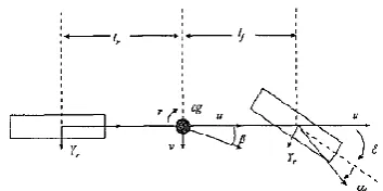
A. Electrical Steering Assist Systems Modelling In [15], a model for the electrical assist system is proposed by Mc Cann et al.. They have used the single track model for the system based on lateral speed 𝑣(𝑡) and Yaw rate 𝑟(𝑡). The state-space equations for these two variables are described as:
2 2
( ) ( ) ( )
( ) ( ) ( )
f r f f r r f
f f r r f f r r f f
c c c
c c c L c L c
dv
v u r
dt mu mu m
c L c L c L c L c L
dr
v r
dt J u J u J
(1)
where 𝑐𝑓 and 𝑐𝑟 are the front and rear tire cornering
coefficients and 𝑢 is the forward component of the vehicle velocity. Fig. 1 indicates the single track model for vehicle dynamics in body centered coordinates. The dynamics of the steering angle 𝛿 are modelled as given in (2).
(
)
(
)
(
)
(
)
3
2
(
)
(
)
f f f
m m
f K SC TB f K SC TB
m m
v K MC
K TB K TB
h h q
m m m
d
w
dt
dw
c d
c L d
v
r
dt
J u
J u
c d G G K
b
G G B
w
J
J
n
K G G
G K
G B
w
i
J
J
J
(2)
where 𝑑 is the caster angle offset distance at the front tires and 𝐽𝑚 is the moment of inertia of the steering system at
the front tire steering axis. 𝐺𝐾, 𝐺𝑆𝐶, and 𝐺𝑀𝐶 are the
mechanical constants relating steering column to front tire torque gain, steering column to the front tire angle ratio, and the assist motor to steering column gear ratio, respectively. The viscous losses associated with the steering gear and ball joints are denoted by 𝑏𝑓. The last
term in (2) is the torque applied to the steering column by the assist motor and gear mechanism. This term is the only control input of the system. The hand wheel dynamics are modelled as:
( ) ( )
( )
h h
SC TB SC TB
h
h h
d TB
h
h h
d w dt
G B G K
dw
w
dt J J
T K
w
J J
(3)
where 𝐾𝑇𝐵 and 𝐵𝑇𝐵 are the torsion bar spring and damping constants, respectively, and 𝑇𝑑 is the torque
which the driver applies to the hand wheel. Consider this value as the torque. The torque sensor measures the angular difference between the hand wheel angle 𝜃ℎ and the steering angle 𝛿 referenced to the steering column. The motor is modelled as a three-phase sinusoidal machine with a permanent magnet rotor. The system has three sensors: The first one measures the difference between the hand wheel angle and the steering shaft angle. The second vehicle measures the lateral acceleration (the derivative of 𝑣), and the third one measures the angular acceleration of the vehicle (the derivative of 𝑟). The last two outputs are exactly our state equations. Moreover, we add 𝐹𝑤 as a disturbance input. Description of the system parameters and their values are presented in [15].
B. Faults Expression
We assume two types of faults for this system: actuator fault and sensor fault. Actuator faults and sensor
faults will cause the alterations in the functionality of the system and the output of the sensors, respectively. To express these faults, we use the standard model proposed in [16]:
( ) ( ) ( ) ( ) ( ) ( ) ( ) ( ) ( )
f d
f d
x Ax t Bu t E f t E d t
y t Cx t Du t F f t F d t
(4)
where the vector f contains both actuator and sensor faults. The 𝐸𝑓is defined as [𝐹0𝑎], and the 𝐹𝑓 matrix is defined as
[𝐹0
𝑠]. 𝐹𝑠 and 𝐹𝑎 are the vectors or the matrices that illustrate
the location of the actuator and sensor faults. We define these two matrices as follows.
First, we define the actuator fault:
0
( ) ( )
f f
u t u t u
(5)
where the matrix Γ is scalar in this situation and 𝐹𝑎 is
considered to be equal to 𝐼. Also, we consider the fault as (𝛼1− 1)𝑢(𝑡) + 𝑢𝑓0. Similarly, for the sensor fault:
0
( ) ( )
f f
y t y t y
(6)
where we choose 𝐹𝑠= 𝐼 and 𝑓𝑠 = (𝐼 − Λ)𝑦 − 𝑦̅̅̅̅𝑓0. For
diagnosing the location of the fault and the extent of its impact, we change Γ and Λ matrices. For example, if we define a fault as 𝑓′= 0.2𝑦2, the second element on the
diameter of the matrix Λ should be 0.8. In addition, by adjusting the 𝑦̅̅̅̅𝑓0 and 𝑢𝑓0 values, we determine the amount of bias. With this explanation, the actuator and sensor faults can be fully defined.
C. Observability And Isolability Of Faults
To check the observability of sensor faults or actuator faults, we will use the following equation:
1
( ) fi fi 0; 1, 2
C sIA E F i
(7)
where i represents the corresponding column of the 𝐸𝑓 and
𝐹𝑓 matrices with the fault. Also, to check the integrity and
isolability of the faults, we study the following Eq. [16]:
1
( ) [ ( )]
l
i i
rank G rank G s
(8)
3.IMPLEMENTATION OF DIFFERENT METHODS
A.Implementation Of Reduced Order Luenberger Observer
Diagnosis observers (DO) are one of the primary and popular methods of fault detection. This is due to their flexible structure and the great similarity of them to the Luenberger observer. The general form of these observers is:
z Gz HuLy Wz Vy Qu
(9)
where 𝑧 ∈ ℛ𝑠 and s can have a reduced degree in comparison with the system degree and this can lead to the design of the reduced degree observer. Although most approaches are based on the reduced degree in observer design, the observer degree is usually bigger than the system degree which is used in optimization. In [16], the lowest possible degree of observer is expressed as:
min
s
(10)
where 𝜎𝑚𝑖𝑛 is the smallest index of the observability
system, which is 2 for electrical steering assist systems; therefore, the lowest possible degree for the Leunberger observer is 2. There are different ways to design the observer, such as algebraic approach [17] and [18] numerical methods. In this paper, we employ the second method.
Algorithm 1. (Numerical methods for the Luenberger observer design)
1) Determine the appropriate amount of s. (𝑠 ≥ 𝜎𝑚𝑖𝑛)
2) Solve the following equation for 𝑣𝑠.
,0 ,
, [ ]
s s s s s
s C
CA
v v v v
CA
(11)
3) Determine the stable matrix G:
1 0
0 0 0
1 0 0
[ ], ,
0 1 0
0 0 1
s
s g
G G g G g R
g
(12)
Specify the L, T, H, Q, V, W matrices using the following equations:
,10 0
1 0 0
0 1 0
0 0 1
s v
T
(13)
Finally, the dynamics of residual producers are:
e Ge
r we
(14)
The results of the implemented observer are studied in Section 4.A.
B. A Fault Detector Implementation Based On The Parity Space Approach
Parity space approach, firstly was introduced by Chow and Willsky in the early 80s [19]. This method is based on a state-space system, but unlike the previous method parity equations are used to produce the residual signal instead of observer. This approach is one of the most important methods for producing the residual signal when is applied to the system in a parallel manner to the observer methods and parameter estimation methods.
In this method, with discretizing the system and writing the output based on the previous states, the number of rows will be added to the observability matrix. Adding these rows may create the null space in the matrix and cause to decrease the matrix rank and make a problem for observability. Also, each of these rows can produce the residual noise.
Defining the following matrices:
, ,
1
( ) ( )
( 1) ( 1)
, ( )
( ) ( )
0 0
0 ,
0
s s
o s u s
s s
y k s u k s
y k s u k s
y u k
y k u k
C D
CA CB D
H H
CA CA B CB D
(15)
The equation of the discrete system can be defined by:
,
,
s o s u s S
y k H x k s H u k
(16)
As a result, the remaining signal can be defined as:
s
s
u s, s
r k v y k H u k
(17)
, 0
s o s
v H
(18)
we have
s
s
u s, s
s o s, 0r k v y k H u k v H
(19)
which indicates the validity of the residual signal definition. However, despite such a structure, the fault detection system does not recognize the difference between the fault and disturbance. To separate fault from disturbance in this method, we should consider the effect of fault and disturbance in the output. Therefore, we define the corresponding matrices to the fault and disturbance as follows:
,
1
,
1
0 0
0 , 0
0 0
0 0
f
f f
f s
s
f f f
d
d d
d s
s
d d d
F
CE F
H
CA E CE F
F
CE F
H
CA E CE F
(20)
with this definition, the output becomes:
, ,
, ,
( ) ( ) ( )
( ) ( )
s o s s u s s
f s s d s s
y k H x k H u k
H f k H d k
(21)
The residual signal can be defined as:
,
,
s S f s S d s S
r k v H f k H d k
(22)
so we need to set the parity vector in the null space of the 𝐻𝑜,𝑠 and 𝐻𝑑,𝑠 matrices, which, having a non-zero
multiplication with 𝐻𝑓,𝑠 matrix. For doing this, solve the
following equation for 𝑣𝑠vectors:
, , 0
s o s d s
v H H
(23)
Then we choose a vector that maximizes the multiplication norm for 𝐻𝑓,𝑠. In these equations, s denotes
the time deep for discretizing. In [20] it is shown that the value of s in the first case (no fault and disturbance isolation) is calculated from:
min
s
(24)
and in the second case the value of s should satisfy:
min max
s
(25)
where 𝜎𝑚𝑖𝑛and 𝜎𝑚𝑎𝑥 are the minimum and maximum index of the observability matrix of the system. In our problem, both indices are equal to 2; therefore, time deep for separating fault from disturbance state is at least 5. To
implement this method, a time moving window with length s will be considered. By moving this window on the data, we calculate and store the residual signal.
As we will see in the simulations, after the occurrence of faults, the residual signal goes back to zero immediately. It may make fault detection more difficult and cause practical disadvantage. To resolve this problem, we have two choices, first we should take advantage of a fast system for fault detection, and the second choice is to slow the time which signal goes to zero using a digital filter. The second solution is to add a filter as:
2 1 0.95H z z
(26)
The simulation of the implementation of this filter is reviewed in Section 4.B. This filter operates on-line and at the same time of producing the residual signal.
C. Implementation Of Decoupling Filter Of Fault From Disturbance
As we discussed before isolation of fault and disturbance is very important. In this section, we intend to design a decoupling filter to separate the fault and disturbance. These filters have a structure similar to conventional observers. The goal of designing such filters is to obtain a vector like 𝑣 vector that meets up both the following equations to omit the effect of the residual signal:
1 1
[ ] 0
[ ] 0
d d d
f f f
vC sI A LC E LF F
vC sI A LC E LF F
(27)
According to a necessary and sufficient condition for decoupling the fault from disturbance is to establish the following inequality:
yf yd yd
rank G G rank G
(28)
There are various methods to implement these filters among which we have used geometric approach in this paper. This method, is first presented. The main idea of this method is to find a matrix such as L which provides maximum uncontrollability in the (𝐴,, 𝐸𝑑, 𝐶) system. To
D.Implementation Of The Unknown Input Observer
The unknown input observer is one type of fault disturbance isolator. This observer has a similar performance to the Luenberger observer. The residual signal in this observer is defined as:
ˆ
r t V yy
(29)
In the late 80s, because of the robust states estimation and robust observer, researchers paid more attention to the unknown input observer approach. The state estimation method in this approach causes that for every input, disturbances and initial values of the system, the value of the estimation error tends to zero. To estimate the states in this approach, we first used a method based on the derivation of the output, but due to the difficulties in implementation they are not considered much. The method which is used in practical problems is as follow given bellow:
Algorithm 2 [23]. (Implementation of fault detector based on the unknown input observer)
Consider the following two conditions.
𝑟𝑎𝑛𝑘(𝐶𝐸𝑑) = 𝑟𝑎𝑛𝑘(𝐸𝑑) = 𝑘𝑑.
(𝐀, 𝐄𝐟, 𝐂) should have no unstable zeros.
If the two conditions have been established, we proceed to the next step.
1) We find 𝑀𝑐𝑒 and T using the following procedure, and then we calculate 𝐿 such that A − LC − E𝑑MceCA is stable.
,
ce d kd kd d ce
M CE I T I E M C
(30)
2) The residual signals are obtained as follows:
(( ) ), 0
( ) ( ) )
d ce
d ce
r v I CE M y Cz v
z TA LC z TA LC E M L y
(31)
The notable point in the implementation of this approach is that because of the structure of the output matrix, the first condition does not meet the required conditions. To remedy this problem, one of the elements in the sixth column of the C matrix is nonzero. It means that we should somehow measure the angular velocity of the steering wheel. Although there is no sensor system, which can measure the angular velocity of the steering wheel in the system, we can calculate that parameter. Thus, by adding a [0 0 0 0 0 1] row in the matrix C, the necessary conditions for designing the filter will be considered. Notice that we can add a 1 into any elements of the sixth column of matrix C, according to the sensor structure of the system it has no physical meaning
to do so. The results of the simulation are shown in Section 4.4.
E. Detection And Reconstruction Of Faults Using Sliding Mode Observer
In fault detection, decoupling and reconstruction of the fault are considered as the highest goal. Fault detectors which we discussed up to now, are only able to detect the occurrence of faults and to distinguish the nature of the disturbance, But those approaches did not comment on the size and type of the fault. In this section, we intend to identify the fault signal using the sliding mode observer.
Fault detection and isolation science done so far. Different approaches conducted in the areas can be divided into four categories:
1) A method based on parameter identification, in which faults are modelled as one of the system parameters;
2) Observers with an extended model which considers the fault as a state variable and design an observer to estimate the states of the system and the faults as well.
3) Adaptive observers which are the combination of the above two approaches.
4) Fault identification filters based on the observers. The difference of these approaches is mainly due to the former information required by each of the four approaches.
In this paper, we used the sliding mode observer which is introduced by Edwards el al. in [24]. In this approach, the following model is considered for the system:
, , ,
f i
o
n n n m p n n q
f
x t Ax t Bu t E f t
y t Cx t f t
A B C E
(32)
In this part, it is assumed that the number of faults will not exceed the total outputs. Moreover, the matrices 𝐶 and 𝐸𝑓are full rank. The goal in this approach is to design an
observer which is able to estimate the states and the output so that the output error tends to zero in some finite time.
ˆ
y
e t y t y t
(33)
Considering the following two conditions:
1) The rank of the matrix is equal to the number of faults.
We can find a transform like 𝑇 which converts the system in the following form:
1 11 1 12 2 1
2 21 1 22 2 2 2
2
i
x A x t A x t B u t
x A x t A x t B u t D f t
y x t
(34)
where 𝑥1∈ ℝ𝑛−𝑝 and 𝑥2∈ ℝ𝑝.
For now, assume that there is no output fault in the system, therefore, the recommended observer has the following form:
1 11 1 12 1 21
21 1 22 2
2
2 2 ,2
22 22 2 ˆ ˆ( ) ˆ ( ) ( ) ( ) ˆ ˆ( ) ˆ ( ) ( ) ( ) ( ) ˆ ( ) y f i s y
x A x t A x t B u t A e t
x A x t A x t B u t E f t
A A e v
y x t
(35)
where 𝐴22𝑠 is a stable designed matrix. The signal 𝑣 is the
injection signal which is obtained from the following equation: 2 ,2 2 y f y P e v E P e
(36)
where 𝑃2 is the answer of the corresponding Lypunov
equation to 𝐴22𝑠 . Moreover, the following inequality applies in the system:
i
f t
(37)
where 𝛿 is a small positive number. It is proved that this observer is asymptotically stable [25].
With performing the sliding motion, the output error and its derivative become zero; thus:
21 1 ,20A e t Ef f ti veq
(38)
where 𝑣𝑒𝑞 is the injection signal corresponding to the
output. This signal denotes the mean behaviour of the input 𝑣 and the control effort needed for sliding movement on the surface. Given our assumption that 𝐴11 is stable, the error will tend to zero, 𝑒1(𝑡) → 0.
Finally, the following important relation will be achieved:
2
eq i
v D f t
(39)
where we can reconstruct the error signal by performing virtual inverse from the injection signal corresponding to the output as follows:
1 2,2 ,2 ,2 ,2 2
y
T T
i f f f f
y P e
f t E E E E
P e
(40)
This signal can be calculated online and only depends on the output estimation error.
To estimate the sensor faults using [9], we can use the following:
1
122 21 11 12
o eq
f A A A A v
(41)
Simulation results in various states are studied in Section 4.
i. Further Details On T Transform
As we discussed before, we used a transformation in designing the observer which classifies the system’s matrix. Edwards in [25] presented an algorithm to compute this transformation, as follows:
1) Represent the matrix C with [𝐶1 𝐶2] where 𝐶2∈ ℝ𝑝×𝑝 and det(𝐶2) ≠ 0. Now, apply the
following transformation to the system so that the output matrix become [0 𝐼𝑝].
1 2 0 n p pre I T C C
(42)
2) Solve the algebraic equation 𝑩𝟏+ 𝑻𝟏𝟐𝑩𝟐= 𝟎 and find 𝑻𝟏𝟐. Determine the orthogonal matrix 𝑻𝟎 so that the following equation is satisfied.
0 20
, m m , det 0
m m
m
T B B B
B
(43)
3) Form the following transformation and apply it on the transformed system 𝑻𝒑𝒓𝒆:
12 0 0 n p I T T T
(44)
The resulting system matrix (𝑨̅) can be classified as:
11 12 22 21 m A A A A A A
(45)
4) Choose the matrix 𝑳 such that 𝑨̅𝟏𝟏+ 𝑳𝑨̅𝒎 is stable. Finally, apply the following transformation to achieve the desired system.
* * 0 0 n p T I L T T
(46)
where 𝐿∗= [𝐿 0(𝑛−𝑝)×𝑚].
To implement this algorithm and determine the 𝑇 transform, we encounter to a problem, because this approach has not provided any method to determine the orthogonal matrix 𝑇0. Although, the 𝑇𝑝𝑟𝑒 transform converts the system to the desired form, the matrix 𝐴11 does not become be stable. To solve this problem, inspired by the example in [24] we changed the structure of the matrix 𝐶 and increased the output to 5. It causes to decrease the size of 𝐴11 to one. If we consider the last five states as the output, the matrix 𝐴11 will become the element of the first row and column of the matrix 𝐴, which is -17.4, that is stable. However, it should also be considered that the structures of matrix 𝐵 and matrix 𝐸𝑓
are in accordance with the problem. If not, we would have to change the rows of matrix 𝐴. Yet, with all these changes and with the assumption that the final 5 states is measurable, this approach reaches to the result as requested. Simulation results are given in Section 4.E.
4.THE SIMULATION STUDY
To simulate this system, we consider two faults. The system has only one input. Therefore, there is only one actuator fault, due to a motor which produces the control signal. This means that, the motor does not work well. The sensor fault is considered to be in the first output, which is the lateral acceleration sensor of automotive. Both faults and disturbances are unknown in nature; thus, without consideration of their physical attribute, we cannot determine their type and size. Here, we assume the size of the fault and disturbance so as they have an equal effect on the output; thus, we can check the performance of each approach. Therefore, two step functions have been considered for the faults and a step function with amplitude of 20 for the disturbances. It is clear that such a value, which can be considered as the value of inserted torque by the driver to the steering system in Newton-meters, is exaggerated. The first disturbance (𝐹𝑤) affects
the system in third seconds, the second disturbance (𝑇𝑑) affects in fifth seconds, the actuator fault occurs in 7th seconds, and sensor fault comes in 9th seconds.
A.Simulation Of Luenberger Observer
Fig. 2 shows the residual signal for the Luenberger observer.
Fig. 2.Residual signal in Luenberger observer approach
The following results can be concluded from Fig.2: 1) The residual signal is sensitive to initial conditions
and input and it needs some time to tend to zero. The time is short and should be passed to the observer for belong able to act.
2) In this observer, faults and disturbances are not distinguished from each other. As we see the second disturbance and actuator fault have the same effect on the residual signal.
3) However, this observer has a lower degree than similar filters have and it requires less computation. As a result, if the effect of the disturbance is not noticeable in the system, the observer works fine for sensor faults.
B. Simulation Of Parity Space Approach
Fig. 3 and Fig. 4 show the generated residual signal of the parity approach in the presence of disturbances and faults, respectively. Fig. 5 and Fig.6 show the same simulation with the filter mentioned in Section C.
Fig. 3.The residual signal in the presence of faults in parity space approach
0 2 4 6 8 10 12
-2 -1.5 -1 -0.5 0 0.5 1 1.5 2 2.5
Time
R
e
s
id
u
a
l
Luenberger Observer-based DO
6 7 8 9 10 11 12
-0.015 -0.01 -0.005 0 0.005 0.01 0.015 0.02
Parity Space Method
Time
R
e
s
id
u
a
l
Fig. 4.The residual signals in the presence of disturbances in parity space approach
Fig. 5.The residual signals in the presence of faults and filter in the parity space approach
Fig. 6.The residual signal in the presence of disturbances and filter in the parity space approach
With comparing these figures we find that:
1) This approach decouples fault from disturbances well. (The amplitude of the fault effect on the
residual noise is several hundred times the effects of disturbance on the residual noise.)
2) Digital filter makes the fault detection much easier and the sensor fault provides a bias in the residual noise.
C. Simulation Of The Decoupling Filter
In this section, the results of the decoupling filter are presented. Figures 7 and 8 show the residual signal in the presence of fault and disturbance, respectively. The results show that the filter can detect the disturbance and separate fault from disturbance.
Fig. 7.The residual signal in the presence of fault in the decoupling filter approach
Fig. 8.The residual signal in the presence of disturbance in the decoupling filter approach
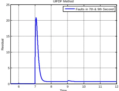
D. Simulation Of Unknown Input Observer The results of the unknown input observer are depicted in Fig. 9 and Fig. 10. It is obvious from Figure 10 that the residual signal has negligible amplitude in the presence of disturbance. The results show that the filter can detect the disturbance and can decouple fault from the disturbance. 0 1 2 3 4 5 6
-4 -3 -2 -1 0 1 2 3 4x 10
-4 Parity Space Method
Time
R
e
s
id
u
a
l
Disturbances in 3th & 5th Second
6 7 8 9 10 11 12
-0.1 0 0.1 0.2 0.3 0.4 0.5 0.6
Parity Space Method with Filter
Time
R
e
s
id
u
a
l
Faults in 7th & 9th Second
0 1 2 3 4 5 6 7 -10
-5 0 5x 10
-3
Parity Space Method with Filter
Time
R
e
s
id
u
a
l
Disturbances in 3th & 5th Second
6 7 8 9 10 11 12
0 5 10 15 20 25
UIFDF Method
Time
R
e
s
id
u
a
l
Faults in 7th & 9th Second
0 1 2 3 4 5 6 -0.5
0 0.5 1 1.5 2 2.5
3x 10
-3 UIFDF Method
Time
R
e
s
id
u
a
l
Fig. 9.The residual signal in the presence of fault in the unknown input observer approach
Fig. 10.The residual signal in the presence of disturbance in the unknown input observer approach
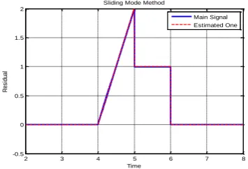
E. Simulation Of Sliding Mode Observer
In this section, the fault reconstruction is presented. So, the actuator fault and sensor fault are considered.
i. Reconstruction Of The Actuator Fault
Fig. 11 shows the estimated actuator fault. Fig. 12 and Fig. 13 show the estimated error and reconstructed fault. In these simulations, we consider 𝜌 = 5 𝑎𝑛𝑑 𝛿 = 0.001. In this observer, two parameters 𝛿and 𝜌 are important, because they can enhance and increase the estimation error and make the system slow.
Fig. 11.Estimation of the actuator fault using sliding mode observer approach
Fig. 12.The 𝒆𝒚 signal
Fig. 13.Reconstructed signal
Fig. 14.Output estimation error
ii. Reconstruction Of Sensor Fault
In this subsection sliding mode observer is used to estimate sensor fault. Fig. 15 shows the reconstructed sensor fault. In this simulation, we consider 𝜌 = 7 𝑎𝑛𝑑 𝛿 = 0.001. In this case, observer is a little sensitive to sudden changes of slope. So it can completely estimate the sensor fault well.
6 7 8 9 10 11 12
-3 -2.5 -2 -1.5 -1 -0.5 0 0.5 1
UIO Method
Time
R
es
id
ua
l
Faults in 7th & 9th Second
0 1 2 3 4 5 6
-6 -5 -4 -3 -2 -1 0 1x 10
-3 UIO Method
Time
R
e
s
id
u
a
l
Disturbances in 3th & 5th Second
2 3 4 5 6 7 8
-0.5 0 0.5 1 1.5 2
Sliding Mode Method
Time
R
es
id
ua
l
Main Signal Estimated One
2 3 4 5 6 7 8
-0.04 -0.035 -0.03 -0.025 -0.02 -0.015 -0.01 -0.005 0 0.005
Sliding Mode Method
Time
R
e
s
id
u
a
l
ey (Estimation Effort
2 3 4 5 6 7 8
-0.5 0 0.5 1 1.5 2
Sliding Mode Method
Time
R
e
c
o
n
s
tr
u
c
te
d
S
ig
n
a
l
Main Signal Estimated One
2 3 4 5 6 7 8
-0.04 -0.035 -0.03 -0.025 -0.02 -0.015 -0.01 -0.005 0 0.005
Sliding Mode Method
Time
O
u
tp
u
t
E
rr
o
r
Fig. 15.Reconstruction of sensor fault using sliding mode observer approach
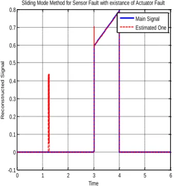
iii. Simultaneous Reconstruction Of Sensor Fault And
Actuator Fault
In this simulation, we apply both faults and investigate the performance of the observer. As we can see in Figs. 16-17, we cannot use single observer for the both faults occurring simultaneously. The reason for this fact is that with a single output error, there is not the possibility of reconstruction of both faults separately. In Fig. 17, the estimator is reconstructing the actuator fault well, but, there is also a response to sensor fault.
Fig. 16.Actuator fault estimation in presence of both faults
Fig. 17.Sensor fault estimation in presence of both faults
iv. Performance In Presence Of Disturbance
Suppose that, we have a disturbance in the output. We examine the detector performance. As we see in Fig. 18, the general performance of the filter disrupts in the presence of the disturbance. It means that, the detector cannot distinguish the difference between fault and disturbance.
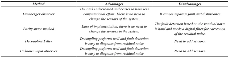
F. Comparison Table
Table 1 compares the four methods of fault detection and presents the advantages and disadvantages of each method.
Fig. 18.Occurrence of the disturbance in the 2nd second and the filter performance
5.CONCLUSION
In this paper, various methods of fault detection for automotive electric steering assist system were studied. According to the results, in general, a parity space approach has the most reasonable answer, because it does not put any additional condition on the system. Therefore, there is no need for change in the system. Yet it does the isolation of the fault and the disturbance well. The last two methods have better performance if there is a possibility of measuring the necessary variables. For more accurate analysis, we can define a threshold and compare the residual noise with the threshold.
2 3 4 5 6 7 8
0 0.1 0.2 0.3 0.4 0.5 0.6 0.7 0.8 0.9 1
Sliding Mode Method
Time
R
ec
on
st
ru
ct
ed
S
ig
na
l
Estimated One Main Signal
0 1 2 3 4 5 6
-8 -6 -4 -2 0 2 4 6 8
Sliding Mode Method for Actuator with existance of Sensor Fault
Time
R
e
c
o
n
s
tr
u
c
te
d
S
ig
n
a
l
Main Signal Estimated One
0 1 2 3 4 5 6 -0.1
0 0.1 0.2 0.3 0.4 0.5 0.6 0.7 0.8
Sliding Mode Method for Sensor Fault with existance of Actuator Fault
Time
R
e
c
o
n
s
tr
u
c
te
d
S
ig
n
a
l
Main Signal Estimated One
0 2 4 6 8 10 12
-4 -3 -2 -1 0 1 2 3 4 5
Sliding Mode Method
Time
R
e
c
o
n
s
tr
u
c
te
d
S
ig
n
a
l
42
Vol. 47 - No. 2 - FallTABLE 1.COMPARISON OF FOUR METHODS OF FAULT DETECTION
Method Advantages Disadvantages
Luenberger observer
The rank is decreased and ceases to have less computational effort. There is no need to
change the sensors of the system.
It cannot separate fault and disturbance
Parity space method Ease of implementation, there is no need to change the sensors in the system.
The fault detection based on the residual noise is hard and needs a digital filter for correction
of the residual noise.
Decoupling Filter Decoupling performs well and fault detection
is easy to diagnose from residual noise Need to add sensors.
Unknown input observer Decoupling performs well and fault detection
is easy to diagnose from residual noise Need to add sensors.
REFERENCES
[1] W. Zhao, Y. Lin, J. Wei, and G. Shi, "Control strategy of a novel electric power steering system integrated with active front steering function," Science China Technological Sciences, vol. 54, pp. 1515-1520, 2011. [2] A. Marouf, C. Sentouh, M. Djemai, and P.
Pudlo, "Control of electric power assisted steering system using sliding mode control," in Intelligent Transportation Systems (ITSC), 2011 14th International IEEE Conference on, 2011, pp. 107-112.
[3] A. Badawy, J. Zuraski, F. Bolourchi, and A. Chandy, "Modeling and analysis of an electric power steering system," SAE Technical Paper 0148-7191, 1999.
[4] A. Gheorghe, A. Zolghadri, J. Cieslak, P. Goupil, R. Dayre, and H. Le Berre, "Model-based approaches for fast and robust fault detection in an aircraft control surface servo loop: From theory to flight tests [applications of control]," Control Systems, IEEE, vol. 33, pp. 20-84, 2013.
[5] J. Zarei, M. A. Tajeddini, and H. R. Karimi, "Vibration analysis for bearing fault detection and classification using an intelligent filter," Mechatronics, vol. 24, pp. 151-157, 2014. [6] Y. Wang, S. Zhang, J. Lu, and F. Chen, "Fault
Detection for Networked Systems with Partly Known Distribution Transmission Delays," Asian Journal of Control, vol. 17, pp. 362-366, 2015.
[7] A. Mehrabian, K. Khorasani, and S. Tafazoli, "Reconfigurable Synchronization Control of Networked Euler‐Lagrange Systems with Switching Communication Topologies," Asian Journal of Control, vol. 16, pp. 830-844, 2014. [8] S. Ahmadizadeh, J. Zarei, and H. R. Karimi,
"Robust unknown input observer design for linear uncertain time delay systems with
application to fault detection," Asian Journal of Control, vol. 16, pp. 1006-1019, 2014.
[9] L. Wang and W. Wang, "H∞ Fault Detection for Two‐Dimensional T‐S Fuzzy Systems in FM Second Model," Asian Journal of Control, vol. 17, pp. 554-568, 2015.
[10] J. Zhang, M. Lyu, H. R. Karimi, and Y. Bo, "Fault detection of networked control systems based on sliding mode observer," Mathematical Problems in Engineering, vol. 2013, 2013. [11] Z. Gao and S. X. Ding, "Actuator fault robust
estimation and fault-tolerant control for a class of nonlinear descriptor systems," Automatica, vol. 43, pp. 912-920, 2007.
[12] R. Isermann, "Diagnosis methods for electronic controlled vehicles," Vehicle System Dynamics, vol. 36, pp. 77-117, 2001.
[13] R. Isermann, R. Schwarz, and S. Stölzl, "Fault-tolerant drive-by-wire systems," Control Systems, IEEE, vol. 22, pp. 64-81, 2002. [14] V. Venkatasubramanian, R. Rengaswamy, K.
Yin, and S. N. Kavuri, "A review of process fault detection and diagnosis: Part I: Quantitative model-based methods," Computers & chemical engineering, vol. 27, pp. 293-311, 2003.
[15] R. McCann, L. Pujara, and J. Lieh, "Influence of motor drive parameters on the robust stability of electric power steering systems," in Power Electronics in Transportation, 1998, 1998, pp. 103-108.
[16] S. Simani, C. Fantuzzi, and R. J. Patton, "Model-Based Fault Diagnosis Techniques," in Model-based Fault Diagnosis in Dynamic Systems Using Identification Techniques, ed: Springer, 2003, pp. 19-60.
[18] S. Ding, E. Ding, and T. Jeinsch, "An approach to analysis and design of observer and parity relation based FDI systems," in Proc. 14th IFAC World Congress, 1999, pp. 37-42. [19] E. Y. Chow and A. S. Willsky, "Analytical
redundancy and the design of robust failure detection systems," Automatic Control, IEEE Transactions on, vol. 29, pp. 603-614, 1984. [20] S. X. Ding, Model-based fault diagnosis
techniques: design schemes, algorithms, and tools: Springer Science & Business Media, 2008.
[21] M.-A. Massoumnia, "A geometric approach to the synthesis of failure detection filters," Automatic Control, IEEE Transactions on, vol. 31, pp. 839-846, 1986.
[22] C. De Persis and A. Isidori, "A geometric approach to nonlinear fault detection and isolation," Automatic Control, IEEE Transactions on, vol. 46, pp. 853-865, 2001. [23] M. Hou and P. Muller, "Disturbance decoupled
observer design: A unified viewpoint," Automatic Control, IEEE Transactions on, vol. 39, pp. 1338-1341, 1994.
[24] C. Edwards, S. K. Spurgeon, and R. J. Patton, "Sliding mode observers for fault detection and isolation," Automatica, vol. 36, pp. 541-553, 2000.