New Learning Methods for Supervised and Unsupervised
Preference Aggregation
Maksims N. Volkovs [email protected]
Richard S. Zemel [email protected]
University of Toronto 40 St. George Street Toronto, ON M5S 2E4
Editor:William Cohen
Abstract
In this paper we present a general treatment of the preference aggregation problem, in which multiple preferences over objects must be combined into a single consensus ranking. We consider two instances of this problem: unsupervised aggregation where no informa-tion about a target ranking is available, and supervised aggregainforma-tion where ground truth preferences are provided. For each problem class we develop novel learning methods that are applicable to a wide range of preference types.1 Specifically, for unsupervised
aggre-gation we introduce the Multinomial Preference model (MPM) which uses a multinomial generative process to model the observed preferences. For the supervised problem we de-velop a supervised extension for MPM and then propose two fully supervised models. The first model employs SVD factorization to derive effective item features, transforming the aggregation problems into a learning-to-rank one. The second model aims to eliminate the costly SVD factorization and instantiates a probabilistic CRF framework, deriving unary and pairwise potentials directly from the observed preferences. Using a probabilistic frame-work allows us to directly optimize the expectation of any target metric, such as NDCG or ERR. All the proposed models operate on pairwise preferences and can thus be applied to a wide range of preference types. We empirically validate the models on rank aggregation and collaborative filtering data sets and demonstrate superior empirical accuracy.
Keywords: preference aggregation, meta-search, learning-to-rank, collaborative filtering
1. Introduction
Many areas of study, such as information retrieval (IR), collaborative filtering, and social web analysis face the preference aggregation problem, in which multiple preferences over objects must be combined into a single consensus ranking. Early developments in preference aggregation and analysis originated in social science (Arrow, 1951) and statistics (Luce, 1959), giving rise to the field of social choice. Research in social choice concentrates on measuring individual interests, values, and/or welfare as an aggregate towards collective decision. Common problems explored in this field include vote aggregation in elections and other domains as well as player/team ranking based on observed game outcomes. Most of these problems are relatively small in size and can be analyzed thoroughly, resulting in models that have well-explored properties and theoretical guarantees. These models
now decide the outcomes of such crucial events as presidential and government elections as well as legal decisions. However, the theoretical guarantees for many of these models typically come at the expense of complicated inference and/or strong assumptions about the preference data (Chevaleyre et al., 2007; Rossi et al., 2011).
The recent explosion of web technologies has generated immense amounts of new pref-erence data. Several properties of this data make it difficult to apply many of the existing aggregation models. First, the ease with which people can access and generate content on the web has resulted in a drastic increase in the quantity of data. For instance, where before the majority of sports data had on the order of a thousand players that participated in several tournaments per year, now, online gaming has millions of users that participate in tens of millions of games daily. Recent statistics on the popular game Halo indicate that over 2 billion multiplayer games are played annually,2 with hundreds of thousands of games happening at any given moment. Consequently, while the aggregation problem in online gaming remains similar to the traditional one in sports—combine preference in the form of game outcomes to generate reliable estimates of players’ skills—any model developed for this task now has to be able to process large amounts of data quickly and handle diverse evidence types ranging from one-on-one games to elimination team tournaments.
Second, the diversity of online applications has led to many new preference types. In addition to the common direct evidence in the form of votes and ratings we now also have a variety of indirect evidence, including web page clicks, dwell time (time spent on a page), and viewing patterns. While these evidence forms do not directly indicate preference, when aggregated across many users, they have been found to closely correlate with it (Joachims, 2002; Joachims et al., 2007). Methods that mine these preferences are now extensively used in search engine optimization (Agichtein et al., 2006; Joachims et al., 2007; Guo et al., 2009) and other domains. Moreover, for some of the new problems the preferences are no longer generated by people. An example of this is meta-search where an issued query is sent to several search engines and the (often partial) document rankings returned by them are aggregated by the meta-search engine to generate more comprehensive ranking results. In this problem there is no human interaction and all the preferences are generated by the machines. Consequently social theories on user behavior and models based on these theories are less applicable here.
Finally, new types of aggregation problems have also recently emerged. In the past the majority of the aggregation problems were unsupervised, that is, no ground truth prefer-ence information about the items was available. For these problems the aim is typically to produce a ranking that satisfies as many of the observed preferences (majority or another related objective) as possible. Due to the popularity of such problems almost all of the ex-isting research in preference aggregation has concentrated on the unsupervised aggregation. However, many of the recent problems are amenable to the supervised setting, as ground truth preference information is available. The meta-search problem mentioned above is one example of supervised preference aggregation. Often, to train/evaluate the aggregat-ing function the documents retrieved by the search engines are given to human annotators who assign relevance labels to each document. The relevance labels provide ground truth preference information about the documents, that is, the documents with higher relevance
label are to be ranked above those with lower one. Another example is crowdsourcing (e.g., MechanicalTurk), where tasks often involve assigning ratings to objects or pairs of objects ranging from images to text. The ratings from several users are then aggregated to produce a single labeling of the data. To ensure consistency in generated labels a domain expert typically labels a subset of the data shown to the “crowd”. The labels are then used to evaluate the quality of annotations submitted by each worker. In these problems the aim is not to satisfy the majority but rather to learn a mapping from the observed preferences to the ground truth ones. Consequently, methods that aim to satisfy the majority often lead to suboptimal results since they lack the “specialization” property: they cannot identify cases where the majority is wrong and only a small subset of the preferences should be used. Such a property is impossible to achieve without referring to the ground truth labels. The scale and variety of the preference data generated by the social and other web domains discussed above show that the field of preference aggregation is rapidly evolving and expanding. Almost every user-oriented web application ranging from web shops and social networks to web search and gaming is now using preference aggregation techniques, the accuracy of which has a direct and significant impact on the generated revenue and business decisions. There is thus an evident need to develop effective aggregation methods that are able to scale to the large web data sets and handle diverse preference types.
As the field has evolved a new trend has recently emerged where machine learning methods are starting to be used to automatically learn the aggregating models. While these methods typically lack the theoretical support of the social choice models they often show excellent empirical performance and are able to handle large and diverse preference data. These models have now been applied successfully to preference aggregation problems in collaborative filtering (Gleich and Lim, 2011; Jiang et al., 2011; Guiver and Snelson, 2009), information retrieval (Cormack et al., 2009; Liu et al., 2007b; Chen et al., 2011) and online gaming (Dangauthier et al., 2007), as well as others. Inspired by these results the work presented in this paper also takes a machine learning approach and develops new models for both supervised and unsupervised preference aggregation problems. In the following sections we describe existing approaches and open challenges for both problems. We then introduce and empirically validate new models for each problem type.
2. Unsupervised Preference Aggregation
expressed in other forms, and where inconsistencies exist in the observed preferences, such as ”a beat b”, ”b beat c”, and ”c beat a”.
In this section we address this problem by developing a flexible probabilistic model over pairwise comparisons. Pairwise comparisons are the building blocks of almost all forms of evidence about preference and subsume the most general models of evidence proposed in literature. Our model can thus be applied to a wide spectrum of preference aggregation problems and does not impose any restrictions on the type of evidence. The score-based approach that we adopt allows for rapid learning and inference, which makes the model applicable to large-scale aggregation problems. We experimentally validate our model on a rank aggregation and collaborative filtering tasks using Microsoft’s LETOR4.0 (Liu et al., 2007a) and the MovieLens (Herlocker et al., 1999) data sets.
2.1 Framework
We assume a set of N instances where for every instance n we have a set of Mn items Xn={xn1, ..., xnMn}and a set of Ψ experts. Each expert ψ∈ {1, ...,Ψ} generates a list of
preferences for items in Xn. We assume that the same set of experts generate preferences
for items in each instance. The preferences can be in the form of full or partial rankings, top-K lists, ratings, relative item comparisons, or combinations of these. All of these forms can be converted to a set ofpartial pairwise preferences, which in most cases will be neither complete nor consistent. We use {xni xnj} to denote the preference of xni over xnj.
We allow the same pairwise preferences to occur multiple times, and use the pairwise count matrixYnψ(i, j) :Mn×Mnto count the number of times preference{xnixnj}is produced
by the expert ψ, withYψn(i, j) = 0 if{xnixnj} is not expressed byψ.
The most straightforward way to convert rankings into pairwise preferences is through binary comparisons. Given two rankings rψni and rψnj assigned by ψ to xni and xnj we set Ynψ(i, j) =I[rψni < rψnj] where I is an indicator function, similarly Ynψ(j, i) =I[rψnj < rniψ].
This representation, however, completely ignores the strength of preference expressed by the magnitude of the rankings. For example, the partial ranking {1,200,300} will have the same count matrix as the ranking{1,2,3}, but the first ranking expresses significantly more confidence about the ordering of the items than the second one. To account for this we instead use Ynψ(i, j) = (rnjψ −rψni)I[rniψ < rψnj] and Ynψ(j, i) = (rniψ −rnjψ)I[rnjψ < rniψ].
In this form we assume that ranking {rni = 1, rnj = 200} is equivalent to observing the
pairwise preference{xnixnj}199 times, whereas ranking{rni = 1, rnj = 2} is equivalent
to observing {xni xnj} only once. This method of accounting for preference strength
is not new and the reader can refer to Gleich and Lim (2011) and Jiang et al. (2011) for more extensive treatment of this and other approaches for converting rankings to pairwise matrices. We summarize these pairwise preference representations below:
1. Binary Comparison:
Ynψ(i, j) =I[rψni< rψnj],
2. Rank Difference:
A ranking of items inXncan be represented as a permutation ofXn. A permutationπ
is a bijection π:{1, ..., Mn} → {1, ..., Mn}mapping each itemxni to its rankπ(i) =j, and i=π−1(j). Given the observed (partial) preference instance nconsisting of count matrices
Yn = {Yn1, ...,YΨn} the goal is to come up with a single ranking π of items in Xn that
maximally satisfies this instance.
Most preference aggregation problems fit this framework. For instance in meta-search instances correspond to queries andXnis the set of documents retrieved for a given queryqn.
Each expertψrepresents a search engine which generates either partial or complete ranking of the documents inXn. As before we can letYnψ(i, j) = (rψnj−r
ψ ni)I[r
ψ ni< r
ψ
nj] if documents xni and xnj are both ranked by the search engine ψ and set Ynψ(i, j) = 0 otherwise. In
collaborative filtering Xis the set of movies/songs/books etc., and an instance of the rank aggregation problem aims to infer the consensus ranking of movies given the (partial) ratings of users ψ (Guiver and Snelson, 2009; Gleich and Lim, 2011). The pairwise approach provides a natural way to model this problem. We can defineYψ(i, j) = (`ψi −`ψj)I[`ψi > `ψj] where`i and `j are the ratings assigned to moviesxni andxnj by userψ. Ifψ did not rate
eitherxni orxnj we set Yψ(i, j) = 0.
2.2 Previous Work
Relevant previous work in this area can be divided into two categories: permutation based and score based. In this section we describe both types of models.
2.2.1 Permutation-Based Models
Permutation based models work directly in the permutation space. The most common and well explored such model is the Mallows model (Mallows, 1957). Mallows defines a distribution over permutations and is typically parametrized by a central permutation σ
and a dispersion parameter φ∈(0,1]; the probability of a permutation π is given by:
P(π|φ, σ) = 1
Z(φ, σ)φ
−D(π,σ),
where D(π, σ) is a distance between π and σ. For rank aggregation problems inference in this model amounts to finding the permutation σ that maximizes the likelihood of the observed rankings. For some distance metrics, such as Kendall’s τ and Spearman’s rank correlation, the partition functionZ(φ, σ) can be found exactly. However, finding the central permutationσ that maximizes the likelihood is typically very difficult and in many cases is intractable (Meila et al., 2007).
A number of other generalizations of the Mallows model such as the Cranking model (Lebanon and Lafferty, 2002) the Aggregation model (Klementiev et al., 2008), and the CPS model (Quin et al., 2010). The Cranking model extends the Mallows distribution to model several diverse preference profiles. Each preference profile i is modeled by its own central permutation σi and ”importance”θi:
P(π|σ,θ) = 1
Z(σ,θ)e −P
iθiD(π,σi),
whereσ ={σi}andθ={θi}are the profile parameters. The above model can be viewed as
a mixture of Mallows models where each component is parametrized by (σi, θi) pair. Using
this alternative representation the work of Klementiev et al. (2008) further generalizes the Cranking model to partial top-K lists and derives an Expectation Minimization (EM) algorithm to learn the parametersθ.
Another recent extension of the Mallows model, the CPS model, defines a sequential generative process, similar to the Plackett-Luce model described below, which draws the items without replacement to form a permutation; the probability of a given permutation
π is:
P(π|σ, φ) =
M Y
i=1
exp(−θP
π1:iD(π1:i, σ))
Z(i, π) ,
where the summation in the numerator is over all permutations π1:i that have the first i
elements fixed toπ;Z(i, π)’s are the normalizing constants that ensure thatP
πP(π|σ, φ) =
1. For several distance metrics such as Spearman’s rank correlation and footrule as well as Kendall’sτ, the summationP
π1:iD(π1:i, σ) over (M−i)! elements, can be found inO(M
2),
allowing the normalizing constants Z(i, π) to be computed in polynomial time. However, during inference one must still consider nearly all of the M! possible permutations to find an optimalπ. A greedy approximation avoids this search, which reduces the complexity to
O(M2), but provides no guarantee with respect to the optimal solution.
In general, due to the extremely large search space (typically M! forM items) and the discontinuity of functions over permutations, exact inference in permutation-based models is often intractable. Thus one must resort to approximate inference methods, such as sampling or greedy approaches, often without guarantees on how close the approximate solution will be to the target optimal one. As the number of items grows, the cost of finding a good approximation increases significantly, which makes the majority of these models impractical for many real world applications where data collections are extremely large. The score-based approach described next avoids this problem by working with real valued scores instead.
2.2.2 Score-Based Models
In score-based approaches the goal is to learn a set of real valued scores (one per item)
Sn={sn1, ..., snMn}which are then used to sort the items. Working with scores avoids the
discontinuity problems of the permutation space.
ranks across the experts or counting the number of pairwise wins. In statistics a very popular pairwise score model is the Bradley-Terry (Bradley and Terry, 1952) model:
P(Yψn|Sn) = Y
i6=j
exp(sni)
exp(sni) + exp(snj)
Ynψ(i,j)
,
where exp(sni)
exp(sni)+exp(snj) can be interpreted as the probability that itemxni beats xnj in the
pairwise contest. In logistic form the Bradley-Terry model is very similar to another pop-ular pairwise model, the Thurstone model (Thurstone, 1927). Extensions of these models include the Elo Chess rating system (Elo, 1978), adopted by the World Chess Federation FIDE in 1970, and Microsoft’s TrueSkill (Dangauthier et al., 2007) rating system for player matching in online games, used extensively in Halo and other games. Furthermore, the popular supervised learning-to-rank model RankNet (Burges et al., 2005) is also based on this approach.
The key assumption behind the Bradley-Terry model is that the pairwise probabilities are completely independent of the items not included in the pair. A problem that arises from this assumption is that if a given itemxnihas won all pairwise contests, the likelihood
becomes larger as sni becomes larger. It follows that a maximum likelihood estimate for sni is ∞ (Mase, 2003). As a consequence the model will always produce a tie amongst
all undefeated items. Often this is an unsatisfactory solution because the contests that the undefeated items participated in, and their opponents’ strengths, could be significantly different.
To avoid some of these drawbacks, the Bradley-Terry model was generalized by Plackett and Luce (Plackett, 1975; Luce, 1959) to a model for permutations:
P(π|Sn) =
Mn
Y
i=1
exp(Sn(π−1(i))) PMn
j=iexp(Sn(π−1(j))) ,
whereSn(π−1(i)) is the score of the item in positioniinπ. The generative process behind
the Plackett-Luce model assumes that items are selected sequentially without replacement. Initially itemπ−1(1) is selected from the set ofMnitems and placed first, then itemπ−1(2)
is selected from the remainingMn−1 items and placed second and so on until allMnitems
model we develop achieves similar improvement over the Plackett-Luce model without the additional computational overhead and preference type restrictions.
Recently several score based approaches have been developed to model the joint pair-wise matrix (Gleich and Lim, 2011; Jiang et al., 2011). In these methods the preferences expressed by each of the experts are combined into a single preference matrix Ytotn = PΨ
ψ=1Y ψ
n, which is then factorized by a low rank factorization such as:
Yntot ≈SneT −eSTn.
The resulting scoresSnare then used to rank the items. The main drawback of this approach is that by combining all preferences into a single Ytotn the individual expert information is lost. Consequently outlier experts with preferences substantially deviating from the consensus can significantly influence both Ytotn and the resulting scores.
2.3 Multinomial Preference Model (MPM)
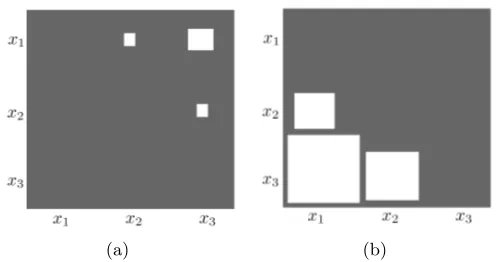
In this section we develop a new score based model for pairwise preferences, the Multinomial Preference Model (MPM) (Volkovs and Zemel, 2012). A key motivating idea behind our approach is that when absolute preferences such as rankings are converted into pairwise counts using the rank difference approach described above, we interpret the resulting counts as conveying two forms of information: a binary preference, simply based on which item is ranked higher, and a confidence, based on the magnitude of the rank difference. Consider for example three items x1, x2 and x3 with ranks r1 = 1, r2 = 2 and r3 = 3 respectively.
Figure 1(a) shows the resulting count matrix after these ranks are converted to pairwise preferences. Item x1 is preferred to both x2 and x3 with Y(1,2) = r2 −r1 = 1 and Y(1,3) =r3−r1 = 2, x2 is preferred only to x3 withY(2,3) =r3−r2 = 1, andx3 is not
preferred to any item. Note that preference{x1 x3}where both items are at the extremes
of the ranking has the largest rank difference and consequently the biggest count.
Now consider the second example with partial ranking r1 = 30, r2 = 20 and r3 = 1
yielding the pairwise count matrix shown in Figure 1(b). Comparing this with the previous example we see that the preference {x3 x1} with items at the extremes of the ranking
also has the highest count, however in this case we are significantly more certain of it. The countY(3,1) = 29 is considerably higher than the highest count from the previous example, strongly indicating thatx3 should be placed abovex1. The two examples demonstrate how
large values of Y(i, j) may be interpreted as providing more evidence to conclude that
{xixj} is correct.
In MPM we model the count matrixYnψ as an outcome of multiple draws from the joint
consensus distributionQn over pairwise preferences defined by the scoresSn. For instance
in the second example above after observing Y we can infer that P(x3 x1) should have
the most mass under Q. We use Bn to denote the random variable distributed as Qn. A
draw fromQncan be represented as a vectorbij of lengthMn∗(Mn−1) (all possible pairs),
with 1 on the entry corresponding to preference{xni xnj}and zeros everywhere else, that
is, a one-hot encoding. GivenSnwe define the consensus distribution as follows:
Definition 1 The consensus distribution Qn = {P(Bn = bij|Sn)}i6=j is a collection of pairwise probabilities P(Bn=bij|Sn), where P(Bn=bij|Sn) = exp(sni−snj)
P
(a) (b)
Figure 1: Figure 1(a) displays the count matrix with the contests won by each of the 3 items x1, x2 and x3 after their ranking{r1 = 1, r2 = 2, r3 = 3} is converted to
pairwise counts using the rank difference method. A count is displayed in each (xi, xj) entry ifri< rj, and the size of the square represents the count magnitude.
Figure 1(b) shows the same matrix for the ranking{r1 = 30, r2 = 20, r3 = 1}.
Qn defines a multinomial distribution over pairwise preferences. Parametrization through Sn controls the shape of Qn, lending considerable flexibility in distributions over
prefer-ences, which can be tailored to many different problems. To generate the observed ag-gregated counts Ynψ we assume that Tnψ independent samples are drawn from Qn where Tnψ =Pi6=jY
ψ
n(i, j) so that:
Yψn(i, j) =
Tnψ
X
t=1
I[Bn=b(t)ij ],
where I[Bn = b(t)ij ] is 1 if preference {xni xnj} was sampled on the t’th draw and 0
otherwise. Under this model the probability of the observed counts is given by:
P(Ynψ|Sn) = T
ψ n! Q
i6=jY ψ n(i, j)!
Y
i6=j
P(Bn=bij|Sn)Yψn(i,j)
= T
ψ n! Q
i6=jY ψ n(i, j)!
Y
i6=j
exp(sni−snj) P
k6=lexp(snk−snl)
!Yψn(i,j)
.
Note that in MPM the pairwise probabilities depend on the entire item set X and the observed counts matrix is modeled jointly. The magnitude of the scoresniis directly related
to the count Yψn(i, j). When the scores are fitted via maximum likelihood the gradient of
the log probability with respect to sni is given by:
∂log(P(Ynψ|Sn)) ∂sni = X j
Yψn(i, j)−X
j
Yψn(j, i)
−Tnψ
∂log(P
k6=lesnk−snl) ∂sni
!
(a) (b)
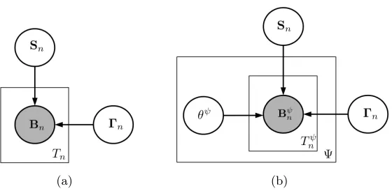
Figure 2: Graphical model representation of the generative process in MPM and its θ ex-tension for a single instance n. Here Tnψ = Pi6=jY
ψ
n(i, j) is the total number
of preferences observed for expert ψ and Tn =PΨψ=1Tnψ is the total number of
preferences across all experts for instancen.
Note that whenxni is strongly preferred to other items the first term in Equation 1 will be
large leading to an increase insni. This will in turn raise the probability of preferences where xni beats the other items. Raising the probability for some preferences must simultaneously
lower it for others since the probabilities always sum to 1. The second term, the derivative of the partition function, accounts for this. The scores thus compete with each other and the ones with the most positive/negative evidence get pushed to the extremes. This is exactly the effect we wanted to achieve because it will allow us to accurately model the count matrices as illustrated by the toy examples above. In contrast with MPM, in the Bradley-Terry model there is no joint interaction amongst scores and pairs are modeled independently so a single preference is sufficient to push the score to infinity.
2.4 Incorporating Prediction Confidence
In the base MPM model it is difficult to judge the model’s confidence for a given score combination. Aside from the relative score magnitudes, it is hard to measure the uncertainty associated with the score assigned to each item and the aggregate ranking that the scores impose. Such a measure can be very useful during inference and can influence the decision process. For instance, it can be used to further filter and/or reorder the items in the aggregate ranking. Moreover, for problems where the accuracy is extremely important, the recommender system can inform the user if the produced ranking has high/low degree of uncertainty.
To address this problem we introduce a set ofvarianceparametersΓn={γn1, ..., γnMn},
γni >0 ∀i. Each γni models the uncertainty associated with the scoresni inferred for the
itemxni. The consensus distribution now becomes:
P(Bn=bij|Sn,Γn) = Pexp((sni−snj)/(γni+γnj)) k6=lexp((snk−snl)/(γnk+γnl))
Note that the probability ofxni beating xnj decreases (increases) if the variance foreither xni or xnj increases (decreases). Through Γn we can effectively express the variance over
the preferences for each itemxni and translate this variance into uncertainty over pairwise
probabilities. Moreover, measures such as the average variance, ¯γn= M1nPMi=1γni, can be
used to infer the variance for the entire aggregate ranking produced by the model.
In this setting the γ’s can either be learned in combination with scores via maximum likelihood or set using some inference procedure. The generative process for MPM with both Sn and Γn parameters is shown in Figure 2(a).
2.5 Modelling Deviations from the Consensus
The assumption in MPM that the preferences generated by the Ψ experts are independent and identically distributed is likely to be false in many domains. Often one would expect to find preferences which either completely or partially deviate from the general consensus. For example in collaborative filtering most people tend to like popular movies such asHarry PotterandForrest Gump, but in almost all cases one can find a number of outlier users who would give these movies low ratings. Assuming that the preferences of the outliers have the same distribution as the consensus, as is done in the base MPM model, can skew the aggregation especially if the outliers are severe.
To introduce the notion of outliers into our model we define an additional set ofadherence
parameters Θ= {θ1, ..., θΨ}, θψ ∈[0,1]. Here we assume that each expert ψ has its own distribution over preferences Qψn, whose adherence to the global consensus distribution Qn
(see Definition 1) is described byθψ. Associated with each expert ψ is a random variable Bψn ∼Qψn, where we define Qψn as:
Qψn ={P(Bψn =bij|Sn,Γn, θψ)}i6=j, P(Bψn =bij|Sn,Γn, θψ) =
exp(θψ(sni−snj)/(γni+γnj)) P
k6=lexp(θψ(sni−snj)/(γni+γnj)) .
Note that if θψ = 0,Qψn becomes a uniform distribution indicating that the preferences of
the expertψdeviate completely from the consensus (is an outlier), and will not be modeled by it. Values between 0 and 1 indicate different degrees of agreement, withθψ = 1 indicating complete agreement. Hence, by introducing θψ we make the model robust, allowing it to control the extent to which each expert’s preferences are modeled by the scores, effectively eliminating the outliers.
In the generative process we now assume that at each of theTn=PψTnψdraws an expert ψis picked at random and a preference is generated fromQψn; Figure 2(b) demonstrates this
Yn={Y1n, ...,YΨn} is given by: P(Yn|Sn,Γn,Θ) =
= Ψ Y ψ=1
Tnψ! Q
i6=jY ψ n(i, j)!
Y
i6=j
P(Bψn =bij|Sn,Γ, θψ)Y
ψ n(i,j) = Ψ Y ψ=1
Tnψ! Q
i6=jY ψ n(i, j)!
Y
i6=j
exp(θψ(sni−snj)/(γni+γnj)) P
k6=lexp(θψ(snk−snl)/(γnk+γnl))
!Ynψ(i,j)
.
The preferences are modeled by a mixture of Ψ multinomials that share the same score vector Sn but differ in the adherence parameter θψ. Both Sn and Θ can be efficiently
learned by maximizing the log likelihood, and the consensus ranking can then be obtained by sorting the scores.
As noted above, in many preference aggregation problems the input typically consists of several preference instances n, and the goal is to infer a separate set of scores Sn and variances Γn for each instance n. The log likelihood of the entire corpus under the model is given by:
L({Yn}|{Sn},{Γn},Θ) =
= log N Y n=1 Ψ Y ψ=1
Tnψ! Q
i6=jY ψ n(i, j)!
Y
i6=j
P(Bψn =bij|Sn,Γ, θψ)Y
ψ n(i,j)
.
Here Θis shared across the instances and the original MPM model is recovered by setting
Θ≡1. When two of the three parameters {Sn,Γn,Θ} are fixed it is not difficult to show that L is concave with respect to the third parameter. Therefore simple gradient descent can be used to efficiently find a globally optimal setting. Furthermore, even though joint optimization is no longer convex, in the experiments we found that by using gradient descent jointly good local optimum solutions can still be found efficiently.
2.6 Rank Aggregation Experiments
For rank aggregation problem we use the LETOR (Liu et al., 2007a) benchmark data sets. These data sets were chosen because they are publicly available, include several baseline results, and provide evaluation tools to ensure accurate comparison between methods. In LETOR4.0 there are two rank aggregation data sets, MQ2007-agg and MQ2008-agg.
MQ2007-agg contains 1692 queries with 69,623 documents and MQ2008-agg contains 784 queries and a total of 15,211 documents. Each query contains several lists of partial rankings of the documents under that query. There are 21 such lists in MQ2007-agg and 25 in MQ2008-agg. These are the outputs of the search engines to which the query was submitted. In addition, in both data sets, each document is assigned one of three relevance levels: 2 = highly relevant, 1 = relevant and 0 = irrelevant. Finally, each data set comes with five precomputed folds with 60/20/20 splits for training/validation/testing. The results shown for each model are the averages of the test set results for the five folds.
The MQ2007-agg data set is approximately 35% sparse, meaning that for an average query the partial ranking matrix of documents by search engines will be missing 35% of its entries. MQ2008-agg is significantly more sparse with the sparsity factor of approximately 65%.
The goal is to use the rank lists to infer an aggregate ranking of the documents for each query which maximally agrees with the held-out relevance levels. To evaluate this agreement we use standard information retrieval metrics: Normalized Discounted Cumulative Gain (N@K) (Jarvelin and Kekalainen, 2000), Precision (P@K) and Mean Average Precision (MAP) (Baeza-Yates and Ribeiro-Neto, 1999). Given an aggregate rankingπ, and relevance levels Ln, NDCG is defined as:
N DCG(π,Ln)@K= 1
G(Ln, K) K X
i=1
2Ln(π−1(i))−1
log(1 +i) ,
where Ln(π−1(i)) is the relevance level of the document in position i in π, and G(Ln, K)
is a normalizing constant that ensures that a perfect ordering has an NDCG value of 1. The normalizing constant allows an NDCG measure averaged over multiple instances with different numbers of items to be meaningful. Furthermore,K is a truncation constant and is generally set to a small value to emphasize the utmost importance of getting the top ranked items correct.
MAP only allows binary (relevant/not relevant) document assignments, and is defined in terms of average precision (AP):
AP(π,Ln) = PMn
i=1P@i∗Ln(π−1(i)) PMn
i=1Ln(π−1(i)) ,
whereP@iis the precision ati:
P@i=
i X
j=1
Ln(π−1(j))
i .
NDCG Precision
N@1 N@2 N@3 N@4 N@5 P@1 P@2 P@3 P@4 P@5 MAP
MQ2008
BordaCount 23.68 28.06 30.80 34.32 37.13 29.72 30.42 29.38 29.75 29.03 39.45 CPS-best 26.52 31.38 34.59 37.63 40.04 31.63 32.27 32.27 31.66 30.64 41.02 SVP 32.49 36.20 38.62 40.17 41.85 38.52 36.42 34.65 32.01 30.23 43.61 Condorcet 35.67 37.39 39.11 40.50 41.59 40.94 37.43 34.73 32.08 29.59 42.63 Bradley-Terry 38.05 39.24 40.77 41.79 42.62 44.77 39.73 36.26 33.19 30.28 44.35
Plackett-Luce 35.20 38.49 39.70 40.49 41.55 41.32 38.96 35.33 32.02 29.62 42.20
θ-MPM 37.07 40.29 41.78 42.76 43.69 43.62 40.94 37.24 33.64 30.81 44.32
MQ2007
BordaCount 19.02 20.14 20.81 21.28 21.88 24.88 25.24 25.69 25.80 25.97 32.52 CPS-best 31.96 33.18 33.86 34.09 34.76 38.65 38.65 38.14 37.19 37.02 40.69 SVP 35.82 35.91 36.53 37.16 37.50 41.61 40.28 39.50 38.88 38.10 42.73 Condorcet 37.31 37.63 38.03 38.37 38.66 43.26 42.14 40.94 39.85 38.75 42.56 Bradley-Terry 39.88 39.86 40.40 40.60 40.91 46.34 44.65 43.48 41.98 40.95 43.98 Plackett-Luce 40.63 40.39 40.26 40.71 40.96 46.93 45.10 43.09 42.32 41.09 43.64
θ-MPM 41.13 41.21 41.09 41.41 41.53 47.35 45.78 44.17 43.01 41.97 44.35
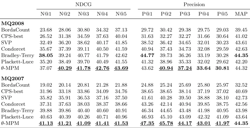
Table 1: MQ2008-agg and MQ2007-agg results; statistically significant results are under-lined.
to 1. All presented NDCG, Precision and MAP results are averaged across the test queries and were obtained using the evaluation script available on the LETOR website.3.
To investigate the properties of MPM we conducted extensive experiments with various versions of the model. Through these experiments we found that theθversion (see Section 2.5) had the best performance; below we refer to this model asθ-MPM. To learn this model we first used the training data to learn the adherence parametersΘ. Then keepingΘfixed we inferred the scores and variances on each test query via maximum likelihood and sorted the scores to produce a predicted ranking. This is similar to the framework used by the CPS model (Quin et al., 2010) where the training data is used to estimate theθparameter. In all experiments we did not take the variances into account during the sort.
We compare the results of θ-MPM against the best methods currently listed on the LETOR4.0 website, namely the BordaCount model and the best of the three CPS models (combination of Mallows and Plackett-Luce models) on each of the MQ data sets. We also compare with the Condorcet, Bradley-Terry and Plackett-Luce models, as well as the sin-gular value decomposition based method SVP (Gleich and Lim, 2011). These models cover most of the primary leading approaches in unsupervised preference aggregation research. The Bradley-Terry model is fit using the same count matrices Yψn that are used for MPM.
For all models we found that 100 steps of gradient descent were enough to obtain the optimal results. To avoid constrained optimization we reparametrized the variance param-eters asγni= exp(βni) and optimizedβni instead. This reparametrization was done for all
the reported experiments.
N@1 N@2 N@3 N@4 N@5 N@6 N@7 N@8 N@9 N@10
Ratings imputed by PMF
Bradley-Terry 40.09 36.00 35.20 34.96 34.49 34.40 31.63 32.08 32.46 32.35 Plackett-Luce 69.56 54.17 48.97 46.58 44.89 43.44 42.50 41.25 40.64 40.03
Neighbor-based 61.48 49.96 44.66 42.87 40.98 39.74 39.01 37.94 37.94 37.73 MPM 69.15 54.29 49.72 46.98 45.52 44.13 43.25 42.62 42.04 41.57
Ratings imputed by neighbor model
Bradley-Terry 34.66 34.07 34.09 34.11 34.02 34.22 32.73 33.14 33.47 33.48 Plackett-Luce 70.81 56.33 50.97 48.27 46.64 45.17 44.17 43.01 42.23 41.74
PMF 69.17 55.93 50.90 48.22 46.65 45.42 44.58 43.88 43.22 42.72
MPM 71.90 56.34 51.21 48.55 46.73 45.41 44.34 43.58 42.94 42.43
Table 2: NDCG results for the MovieLens data set, for each user the missing ratings are filled using the probabilistic matrix factorization model (top half), and the neighbor-based approach (bottom half); statistically significant results are under-lined.
The results4 for MPM together with the baselines on MQ2008-agg and MQ2007-agg data sets are shown in the top and bottom halves of Table 1 respectively. For each data set we conducted a paired T-test between θ-MPM and the best baseline at each of the 5 truncations for NDCG and precision as well as MAP; the statistically significant results at the 0.05 level are underlined.
From the table we see that the θ-MPM models significantly outperforms the baselines on the MQ2007-agg data set on both NDCG and MAP metrics. θ-MPM is also the best model On MQ2008-agg, significantly improving over the baselines on truncations 2-5 for NDCG and 2,3 for Precision.
2.7 Collaborative Filtering Experiments
For collaborative filtering experiments we used the MovieLens data set,5 a collection of
100,000 ratings (1-5) from 943 users on 1682 movies. This data set was chosen because it provides demographic information such as age and occupation for each user, as well as movie information such as genre, title and release year. Each user in this data set rated at least 20 movies, but the majority of ratings for each movie are missing and the rating matrix is more than 94% sparse. We formulate the preference aggregation as follows: given users’ ratings the goal is to come up with a single ranking of the movies that accurately summarizes the majority of user preferences expressed in the data. This ranking could be used as an initial recommendation for a new user who has not provided any ratings yet, as well as in a summary page. Note that the aggregation can be further personalized by only aggregating over users that share similar demographic and/or other factors with the target user.
4. All NDCG and precision values in this and other tables were multiplied by 100 to make them more readable.
To convert ratings into preferences we can either sort them (resolving ties), to obtain a partial ranking for each user, or use the pairwise method to obtain the count matrices
Yψ, where Yψ(i, j) = (`ψi −`ψj)I[`ψi > `ψj] if movies xi and xj were rated by user ψ and 0
otherwise. We use the sort method for the permutation-based Plackett-Luce model and use the rating difference method for the pair-based Bradley-Terry and MPM models.
In collaborative filtering and in most other applications the primary goal of aggregation is to recommend items to a new or existing user. Items ranked in the top few positions are of particular interest because they are the ones that will typically be shown to the user. Intuitively a top ranked item should have ratings from many users (high support) and most who rated it should prefer it to other items (strong preference). Consequently NDCG is a good metric to evaluate the rankers for this problem because of its emphasis on the top ranked items and the truncation level structure. Unlike rank aggregation the ground truth aggregate ratings are not available for most collaborative filtering data. To get around this problem we complete the rating matrix by imputing the missing ratings for every user. We investigate two methods of imputing the ratings: a user independent method, where all the missing ratings are filled in by the same value, and two user dependent methods. The first method is neighbor-based and predicts the ratings using the nearest neighbors for a given userψ. The second method uses the probabilistic matrix factorization model (PMF) (Salakhutdinov and Mnih, 2008) to factorize the rating matrix and predict missing entries. Both are commonly used for CF and have shown good empirical performance on various CF tasks such as the Netflix challenge. After completing the rating matrix we compute the NDCG value for every user by sorting the items according to scores:
N DCG(π,Lψ)@K = 1
G(Lψ, K) K X
i=1
2Lψ(π−1(i))−1
log(i+ 1) . (2)
Here π is the aggregated ranking obtained by sorting the items according to scores, and
π−1(i) is the index of the item in position iinπ;Lψ is a (completed) vector of ratings for userψ. G(Lψ, K) is the normalizing constant and represents the maximum DCG value that could be obtained forψ:
G(Lψ, K) =
K X
i=1
2Lψ(σ−i(i))−1 log(i+ 1) ,
where σ is a permutation of Lψ with the ratings sorted from largest to smallest. In this form, if an item in position i in π has a rating lower than the rating Lψ(σ−1(i)) of the
i’th highest rated item by user ψ, the corresponding term in the NDCG summation will decrease exponentially with the difference betweenLψ(σ−1(i)) andLψ(π−1(i)). We use this metric (averaged across all users) to evaluate the performance of the models.
(a) (b) (c)
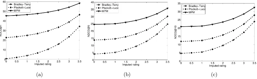
Figure 3: Plots of NDCG at truncations 1, 5 and 10; in this setting all the missing ratings were repeatedly imputed by one of the constants shown on the x-axis and the rankings given by each method were evaluated using NDCG (Equation 2). All the differences are statistically significant.
vector for each user to get a user-dependent item ranking. The resulting rankings are then aggregated across all users using the Borda rule. We chose to use Borda count here because it is a well-explored approach that has stable performance and is commonly applied to social choice problems such as CF.
The NDCG results from the user dependent rating imputation method are shown in Table 2. From this table we see that MPM outperforms the best aggregation method, Plackett-Luce, both when ratings are imputed by the neighbor-based approach (top half of the table) and PMF (bottom half of the table). We also see that the neighbor-based CF model performs considerably worse than both MPM and Plackett-Luce while PMF has competitive performance, outperforming MPM at higher truncations. These results are consistent with the CF literature where PMF is typically found to perform better since it can capture more complex correlations that extend beyond simple neighbor relationships. However, unlike most aggregation methods that only learn one parameter (two for MPM) per item, in PMF we have to fit a set of parameters for each user and item. This significant increase in the number of parameters makes optimization more complex as PMF models are typically highly prone to overfitting. Moreover, it is unclear how learned models should be used to get the aggregate ranking as they only provide user-dependent rating predic-tions. This introduces an additional optimization step that needs to be run before ranking predictions can be made. Overall, for the MovieLens data we found that these models did not give significant gains while being considerably slower.
Bradley-Terry #u #won #lost Plackett-Luce #u #won #lost MPM #u #won #lost Pather Panchali 8 1431 89 Shawshank Red. 283 32592 5943 Star Wars 583 49290 10112 Wallace & Gromit 67 7448 962 Wallace & Gromit 67 7448 962 Raiders of the L. 420 40057 10644 Casablanca 243 26837 4633 Usual Suspects 267 30779 6666 Godfather 413 36531 8040 Close Shave 112 11219 1963 Star Wars 583 49290 10112 Silence of the L. 390 38192 9125 Rear Window 209 22590 4513 Wrong Trousers 118 13531 2291 Shawshank Red. 283 32592 5943
. . .
. . .
. . .
Children of Corn 19 62 3161 Barb Wire 30 462 5507 Cable Guy 106 3469 14377 Lawnmower Man 2 21 129 3868 Robocop 3 11 125 2535 Striptease 67 1347 9909 Free Willy 3 27 171 3912 Gone Fishin’ 11 123 1098 Very Brady 93 3353 12509 Kazaam 10 128 2041 Highlander III 16 881 2826 Jungle2Jungle 132 2375 11086 Best of the Best 3 6 33 1445 Ready to Wear 18 289 3785 Island of Dr. 57 1176 9415
Table 3: Top 5 and bottom 5 movies found by each model. For each movie the table shows the number of users that rated it (#u) and the total number of pairwise contests that the movie won (#won) and lost (#lost) across all users.
higher than the average of the unobserved ones (Marlin et al., 2005). From the figure we see that MPM significantly outperforms both the Bradley-Terry and Plackett-Luce models. The differences are especially large when low values are imputed for the missing ratings. This indicates that the Bradley-Terry and Plackett-Luce models place items that were rated by very few users (low support) at the top of the list. This causes the imputed ratings to dominate the numerator in the NDCG summation making the results very sensitive to the magnitude of the imputed rating.
This effect can also be observed from Table 3, which shows the top and bottom 5 movies generated by each model together with statistics on the number of users that rated each movie and the number of pairwise contests lost and won by the movie (summed across all users). For a given user ψand moviei with rating`ψi we find the number of pairwise wins by counting the number of pairs (i, j) with`ψi > `ψj; losses are found in a similar way. From the table we see that the Bradley-Terry model places the moviePather Panchaliat the top of the list. This movie is only rated by 8 out of 943 users and even though most users who rated it preferred it to other movies (#lost is low) there is still very little evidence that this movie represents the top preference for the majority of users. Due to its pairwise independence assumption the Bradley-Terry model is always likely to place movies with few ratings near the top/bottom of the list.
The Plackett-Luce model partially fixes this problem by considering items jointly, and places the frequently rated movie Shawshank Redemption first. However the model does not fully eliminate the problem, placing the very infrequently ratedWallace & Gromit(also ranked second by Bradley-Terry) in the second spot. Part of the reason for this comes from the fact that Plackett-Luce is a permutation based model and as such cannot model the strength of preferences, treating the preferences given for example by ratings {5,2,1} the same as{5,4,3}.
(a) (b)
Figure 4: 4(a) shows the number of ratings versus the learned variance γi for each movie xi. 4(b) shows the rank for each movie obtained after sorting the scores versus
the learnedγi.
preference. The top three movies are all rated by more than 400 users and are strongly preferred by the majority of those users.
A more severe pattern can be observed for the bottom 5 movies. Both Bradley-Terry and Plackett-Luce place movies rated by fewer than 30 users in the bottom 5 positions, labeling them the worst movies in the entire data set. This selection has very little evidence in the data and has a high probability of being wrong if more ratings are collected. For MPM all of the bottom 5 movies are rated by more than 50 users with 3 out of 5 movies rated by more than 90 users.
In addition to the retrieval accuracy we investigated the properties of the learned vari-ance parameters γ. Figure 4(a) shows the learned variances together with the number of ratings for each movie. Note that the variance is inversely proportional to the number of ratings, so as the number of ratings increases the model becomes increasingly more certain in the preferences, decreasing the variance. In Figure 4(b) we plot γ against the aggre-gate rank for each movie. The general pattern is clear: the variance decreases towards the extremes of the ranking, indicating that the model is more certain in the movies that are placed near the top and near the bottom of the aggregate ranking. As shown above, this is due to the fact that the movies at the extremes of the ranking have many comparisons, allowing accurate inference of strong negative or positive preferences.
disliked. The model thus appropriately placed them in the middle of the ranking with strong confidence. Moreover, note that it is impossible to express this confidence with scores alone since all the movies in the middle of the ranking have similar scores. The variances thus provide additional information about the decisions made by the model during the aggregation, which could be very useful for post-processing and evaluation.
3. Supervised Preference Aggregation
Research in preference aggregation has largely concentrated on the unsupervised aggregation problem described above. However, many of the recent aggregation problems are amenable to supervised learning, as ground truth preference information is available. The meta-search and crowdsourcing problems are both examples of supervised preference aggregation. Due to the popularity of these and other supervised problems the supervised aggregation framework has received a lot of attention recently, with a number of competitions conducted in TREC6
as well as other conferences, and several meta-search data sets(Liu et al., 2007a) have been released to encourage research in the area. Despite these efforts, to the best of our knowledge most of the proposed models are still unsupervised and the supervised methods are unable to fully use the labeled data and optimize the aggregating function for the target metric. There is thus an evident need to develop an effective supervised aggregation framework.
To address this problem we first develop a supervised extension of the MPM model introduced in the previous section. We show how the labeled training data can be used to set the adherence parametersΘand experimentally verify that this approach improves the test accuracy of the model.
We then develop a general framework for supervised preference aggregation. Our frame-work builds on the idea of converting the observed preferences into pairwise matrices de-scribed in the previous section. We first show how these matrices can be used to derive effective fixed length item representations that make it possible to apply any learning-to-rank method to optimize the parameters of the aggregating function for the target IR metric. We then show how the pairwise matrices can also be employed as potentials in a ranking Conditional Random Field (CRF), and develop efficient learning and inference procedure to optimize the CRF for the target IR metric.
We validate all of the introduced models on two supervised rank aggregation data sets from Microsoft’s LETOR4.0 data collection.
3.1 Framework
As in unsupervised preference aggregation, a typical supervised problem also consists of training instances where for each instance we are given a set of items. The experts generate preferences for the items and the preferences can be in the variety of forms ranging from full/partial rankings and ratings to relative item comparisons and combinations of these. However, unlike the unsupervised problem, we now also have access to the ground truth preference information over the items for each instance. The goal is to learn an aggregating function which maps expert preferences to an aggregate ranking that maximally agrees with the ground truth preferences.
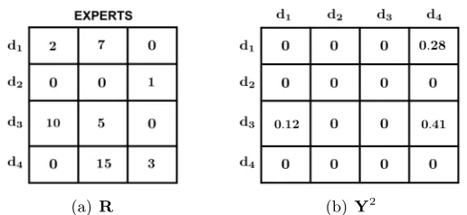
(a)R (b) Y2
Figure 5: (a) An example rank matrixRwhere 4 documents are ranked by 3 experts. Note that in meta-search the rank for a given document can be greater than the number of documents in R. (b) The resulting pairwise matrix Y2 for expert 2 (second column of R) after the ranks are transformed to pairwise preferences using the log rank difference method.
In this work we concentrate on the rank aggregation instance of this problem from the information retrieval domain. However, the framework that we develop is general and can be applied to any supervised preference aggregation problem in the form defined above. In information retrieval the instances correspond to queries Q={q1, ..., qN} and items to
documents Dn = {dn1, ...., dnMn} where Mn is the number of documents retrieved for qn.
For each query qn the experts’ preferences are summarized in an Mn×Ψ rank matrix Rn
whereRn(i, ψ) denotes the rank assigned to document dni by the expertψ. Note that the
same Ψ experts rank items for all the queries so Ψ is query independent. Furthermore,
Rn can be sparse, as experts might not assign ranks to every document in Dn; we use
Rn(i, ψ) = 0 to indicate that document dni was not ranked by expert ψ. The sparsity
arises in problems like meta-search where qn is sent to different search engines and each
search engine typically retrieves and ranks only a portion of the documents in Dn. The ground truth preferences are expressed by the relevance levels Ln ={`n1, ..., `nMn} which
are typically assigned to the documents by human annotators.
In contrast to the learning-to-rank problem where each document is represented by a fixed length, query dependent, and typically heavily engineered feature vector, in rank aggregation the rank matrix R is the only information available to train the aggregating function. Additionally this matrix is typically very sparse. Hence there is no fixed length document description, as is required by most supervised methods. To overcome this problem we use the ideas behind the MPM approach and convert the rank matrix into a pairwise preference matrix. We then show how this conversion can be used to develop an effective supervised framework for this problem.
3.2 Pairwise Preferences
Given the Mn×Ψ ranking matrix Rn our aim is to convert it into Ψ Mn×Mn pairwise
matrices Yn = {Yn1, ...,YnΨ}, where each Ynψ expresses the preferences between pairs of
transformations; here we extend these ideas and consider a general transformation of the form Ynψ(i, j) =g(Rn(i, ψ),Rn(j, ψ)). We experiment with three versions for g that were
proposed by Gleich and Lim (2011): Binary Comparison (Equation 1), and normalized and logarithmic versions of Rank Difference (Equation 2).
3. Normalized Rank Difference
Here the normalized rank difference is used:
Ynψ(i, j) =I[Rn(i, ψ)<Rn(j, ψ)]
Rn(j, ψ)−Rn(i, ψ)
max(Rn(:, ψ)) .
Normalizing by the maximum rank assigned by the expertψ(max(Rn(:, ψ))) ensures that the entries of Yψn have comparable ranges across experts.
4. Log Rank Difference
This method uses the normalized log rank difference:
Ynψ(i, j) =I[Rn(i, ψ)<Rn(j, ψ)]
log(Rn(j, ψ))−log(Rn(i, ψ))
log(max(Rn(:, ψ))) .
In all cases both Yψn(i, j) and Yψn(j, i) are set to 0 if either Rn(i, ψ) = 0 or Rn(j, ψ) = 0
(missing ranking). Non-zero entriesYψn(i, j) represent the strength of the pairwise
prefer-ence {dni dnj} expressed by expert ψ. Figure 5 shows an example ranking matrix and
the resulting pairwise matrix after the ranks are transformed to pairwise preferences using the log rank difference method. Note that preferences in the form of ratings and top-K lists can easily be converted intoYψn using the same transformations. Moreover, if pairwise
preferences are observed, we simply skip the transformation step and fill the entriesYψn(i, j)
directly.
As mentioned above, working with pairwise comparisons has a number of advantages, and models over pairwise preferences have been extensively used in areas such as social choice (David, 1988), information retrieval (Joachims, 2002; Burges, 2010), and collaborative filtering (Lu and Boutilier, 2011; Gleich and Lim, 2011). First, pairwise comparisons are the building blocks of almost all forms of evidence about preference and subsume the most general models of evidence proposed in literature. A model over pairwise preferences can thus be readily applied to a wide spectrum of preference aggregation problems and does not impose any restrictions on the input type. Second, pairwise comparisons are a relative measure and help reduce the bias from the preference scale. In meta-search for instance, each of the search engines that receives the query can retrieve diverse lists of documents significantly varying in size. By converting the rankings into pairwise preferences we reduce the list size bias emphasizing the importance of the relative position.
3.3 Previous Work
In meta-search a heuristic method called Reciprocal Rank Fusion (RRF) (Cormack et al., 2009) has recently been proposed. RRF uses the rank matrix to derive the document scores:
sni= Ψ X
ψ=1
1
α+Rn(i, ψ),
where α is a constant which mitigates the impact of high rankings from outlier experts and is set by cross validation. Once the scores are computed they are used to sort the documents. We place this method into the supervised category because of the need to set the constant α which has a significant effect on ranking accuracy (Cormack et al., 2009). Despite its simplicity RRF has obtained excellent empirical accuracy; however it also has some disadvantages. First, RRF relies on complete rankings and it is unclear how to extend it to problems like meta-search where many rankings are typically missing. Second, this method is designed specifically for rank aggregation and cannot be applied to other types of preferences.
A supervised score-based rank aggregation approach based on a Markov Chain was also recently introduced by Liu et al. (2007b). In this model the authors use the ground truth preferences to create a pairwise constraint matrix and then learn a scoring function such that the produced aggregate rankings satisfy as many pairwise constraints as possible. The main drawbacks of this approach are that it is computationally very intensive, requiring constrained optimization (semidefinite programming), and it does not incorporate the target IR metric into the optimization. The pairwise constraint idea was also recently extended by Chen et al. (2011) to a semi-supervised setting where the ground truth preferences are available for only a subset of the documents.
Extensive work in the learning-to-rank domain has demonstrated that optimizing the ranking function for the target metric produces significant gains in test accuracy (Li, 2011). However, to the best of our knowledge none of the models developed for supervised prefer-ence aggregation take the target metric into account during the optimization of the aggre-gating function. The models that we develop in the following sections aim to bridge this gap.
3.4 Supervised Extension for MPM
Before delving into the new models we first develop a simple supervised extension for the Multinomial Preference Model introduced above. The MPM can be considered fully un-supervised, as the adherence parameters Θ, the consensus scores and the variances are inferred from the observed preferences. This produces a predicted ranking for a given set of observed preferences by sorting the inferred scores, without ever using any known con-sensus rankings or relevance labels in the data. In this section we describe an approach to incorporate this ground truth information into this model.
expertψ and the ground truth labels across the instances:
θψ = 1
N N X
n=1
1− D(Ln,Yψn),
where D is a normalized distance metric between preferences, such as Kendall’s τ. Note thatθψ →1(→0) indicates that the preferences of expertψ agree with (deviate from) the ground truth preferences (target consensus) across the training examples.
To apply the model we now (1) use the labeled training instances to find Θ and (2) keepingΘfixed infer scores and variances for each test instance by maximizing the likelihood of the observed preferences.
3.5 Feature-Based Approach
We now introduce the first of the two fully supervised models for preference aggregation. The main idea behind this approach is to summarize the relative preferences for each doc-ument across the experts by a fixed length feature vector (Volkovs et al., 2012). This transforms the preference aggregation problem into a learning-to-rank one, and any of the standard methods can then be applied to optimize the aggregating function for the tar-get IR metric such as NDCG. In following section we describe an approach to extract the document features.
3.5.1 Feature-Based Approach: Feature Extraction
Given the rank matrix Rn and the resulting pairwise matrix Yψn for expert ψ (as shown
in Figure 5), our aim is to convert Yψn into a fixed length feature vector for each of the
documents in Dn. Singular Value Decomposition (SVD) based approaches for document
summarization such as Latent Semantic Indexing (Deerwester et al., 1990) are known to produce good descriptors even for sparse term-document matrices. Another advantage of SVD is that it requires virtually no tuning and can be used to automatically generate the descriptors once the pairwise matrices are computed. Because of these advantages we chose to use SVD to extract the features. For a given Mn×Mn pairwise matrix Yψn the rank-p
SVD factorization has the form:
Ynψ ≈UψnΣψnVnψ,
whereUψn is anMn×pmatrix,Σψn is anp×p diagonal matrix of singular values andVnψ is
anMn×pmatrix. The full SVD factorization hasp=Mn, however, to reduce the noise and
other undesirable artifacts of the original space most applications that use SVD typically set p Mn. Reducing the rank is also an important factor in our approach as pairwise
matrices tend to be very sparse with ranks significantly smaller than Mn.
Given the SVD factorization we use the resulting matrices as features for each document. It is important to note here thatbothUψn andVψn contain useful document information since Ynψ is a pairwise document by document matrix. To get the features for documentdni and
expertψ we use:
φ(dni,Ynψ) = [Uψn(i,:),diag(Σψn),Vψn(i,:)],
hereUψn(i,:) and Vnψ(i,:) are the i’th rows of Uψn andVnψ respectively and diag(Σψn) is the
independent ofiand will be the same for all the documents inDn. We include the singular
values to preserve as much information from the SVD factorization as possible. The features
φ(dni,Yψn) summarize the relative preference information fordniexpressed by the expertφ.
To get a complete view across the experts we concatenate together the features extracted for each expert:
φ(dni) = [φ(dni,Yn1), ..., φ(dni,YnΨ)].
Each φ(dni,Yψn) contains 3p features so the entire representation will have 3Ψp features.
Moreover, note that since the experts and p are fixed across queries this representation will have the same length for every document in each query. We have thus created a fixed length feature representation for every document dni, effectively transforming the
aggregation problem into a standard learning-to-rank one. During training our aim is now to learn a scoring function f : R3Ψp → R which maximizes the target IR metric such as
NDCG. The feature representation allows us to fully use all of the available labeled training data to optimize the aggregating function for the target metric, which is not possible to do with the existing aggregation methods.
It is worth mentioning here that the SVD factorization of pairwise matrices has been used in the context of preference aggregation (see (Gleich and Lim, 2011) for example). However, previous approaches largely concentrated on applying SVD to fill the missing entries in the joint pairwise matrixYntot=PΨ
ψ=1Y ψ
n and then use the completed matrix to
infer the aggregate ranking. Our approach on the other hand uses SVD to compress each pairwise matrixYnψ and produce fixed length feature vector for each document.
3.5.2 Feature-Based Approach: Learning and Inference
Given the document features extracted via the SVD approach our goal is to use the labeled training queries to optimize the parameters of the scoring function for the target IR metric. The main difference between the introduced feature-based rank aggregation approach and the typical learning-to-rank setup is the possibility of missing features. When a given documentdni is not ranked by the expertψ the rowYψn(i,:) and column Yψn(:, i) will both
be missing (i.e., 0). To account for this we modify the conventional linear scoring function to include a bias term for each of the Ψ experts:
f(φ(dni),W) = X
ψ∈Ψ
wψ·φ(dni,Ynψ) +I[Rn(i, ψ) = 0]bψ, (3)
where W = {wψ, bψ}ψ is the set of free parameters to be learned with each wψ having the same dimension as φ(dni,Ynψ), and I[] is an indicator function. The bias term bψ
provides a base score fordni ifdni is not ranked by expertψ. The weights wψ control how
Algorithm 1 Feature-Based Learning Algorithm
Input: {(q1,D1,L1,R1), ...,(qN,DN,LN,RN)} Parameters: learning rateη
for n= 1 toN do{feature extraction}
fromRncompute Yn={Y1n, ...,YΨn} fori= 1 toMn do
compute features φ(dni) using SVD end for
end for
initialize weights: W
repeat {scoring function optimization}
forn= 1 to N do
computeλ-gradients: ∇W=P
iλni∂s∂Wni
update weights: W=W−η∇W end for
until convergence
Output: W
LambdaRank here and refer the reader to Burges et al. (2006) and Burges (2010) for a more extensive treatment.
LambdaRank learns pairwise preferences over documents with emphasis derived from the NDCG gain found by swapping the rank position of the documents in any given pair, so it is a listwise algorithm (in the sense that the cost depends on the sorted list of documents). Formally, given a pair of documents (dni, dnj) with `ni 6= `nj, the target probability that dni should be ranked higher thandnj is defined as:
Pnij =
1 if `ni > `nj
0 otherwise .
The model’s probability is then obtained by passing the difference in scores between dni
and dnj through a logistic:
Qnij =
1
1 + exp(−(f(φ(dni),W)−f(φ(dnj),W)))
= 1
1 + exp(−(sni−snj)) .
The aim of learning is to match the two probabilities for every pair of documents with different labels. To achieve this a cross entropy objective is used:
On=− X
`ni>`nj
Pnijlog(Qnij).
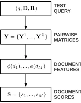
Figure 6: The inference diagram for the feature-based preference aggregation approach. Given a test query (q,D,R) the inference proceeds in three steps: (1) The ranking matrixR is converted to a set of pairwise matrices Y={Y1, ...,YΨ}. (2) SVD is used to extract document features from each pairwise matrix Yψ. (3) The learned scoring function is applied to the features to produce the scores for each document. The scores are then sorted to get the aggregate ranking.
on the top of the ranking. To take this into account the LambdaRank framework uses a smooth approximation to the gradient of a target evaluation measure with respect to the score of a documentdni, and we refer to this approximation asλ-gradient. Theλ-gradient for
NDCG is defined as the derivative of the cross entropy objective weighted by the difference in NDCG obtained when a pair of documents swap rank positions:
λnij =|∆N DCG@K(sni, snj)|
∂On ∂(sni−snj)
.
Thus, at the beginning of each iteration, the documents are sorted according to their current scores, and the difference in NDCG is computed for each pair of documents by keeping the ranks of all of the other documents constant and swapping only the rank positions for that pair (see Burges et al., 2006 for more details onλcalculation). Theλ-gradient for document
dni is computed by summing the λ’s for all pairs of documents (dni, dnj) for queryqn:
λni= X
j:`nj6=`ni
λnij.
The|∆N DCG|factor emphasizes those pairs that have the largest impact on NDCG. Note that the truncation in NDCG is relaxed to the entire document set to maximize the use of the available training data.
complexity at the cost of additional storage requirement of O(MnΨp) for each query qn.
The complete stochastic gradient descent learning procedure is summarized in Algorithm 1.
Once the parameters of the scoring function are learned then at test time, given a new query q with rank matrix R, we (1) convert R into a set of pairwise matrices Y =
{Y1, ...,YΨ}; (2) extract the document features using rank-pSVD; and (3) apply the learned scoring function to get the score for every document. The scores are then sorted to get the aggregate ranking. This process is shown in Figure 6.
3.6 CRF Approach
The SVD-based feature approach introduced above is effective at producing compact doc-ument representation which we experimentally found to work well for this task. These representations also allow to apply any learning-to-rank approach making it very easy to incorporate the model into many existing IR frameworks. However, while the SVD model is robust, it requires applying SVD factorization at test time which can be computation-ally intensive. Moreover, SVD representation significantly compresses the pairwise matrices and might throw away useful information potentially affecting performance and making the model less interpretable. To avoid these disadvantages we develop another fully supervised model which uses the pairwise matrices directly. As mentioned above, the variable number of documents per query and absence of the fixed-length document representation make it difficult to apply the majority of supervised methods to this problem, since they require fixed-length item representations. CRFs on the other hand are well suited for tasks with variable input lengths, and have successfully been applied to problems that have this prop-erty, such as natural language processing (Sha and Pereira, 2003; Roth and Yih, 2005), computational biology (Sato and Sakakibara, 2005; Liu et al., 2006), and information re-trieval (Qin et al., 2008; Volkovs and Zemel, 2009). Moreover, CRFs are very flexible and can be used optimize the parameters of the model for the target metric. For these reasons we develop a CRF framework for preference aggregation (Volkovs and Zemel, 2013).
3.6.1 CRF Approach: Model
The main idea behind this approach is based on an observation that the pairwise preference functions defined above naturally translate to pairwise potentials in a CRF model. Using these function we can evaluate the “compatibility” of any rankingπ by comparing the order induced by the ranking with the pairwise preferences from each expert. This leads to an energy function:
E(π,Yn;W) =
=− 1
M2
n Mn
X
i=1 PΨ
ψ=1
bψϕψ(π−1(i)) +wψ pos
P
j6=iY ψ
n(π−1(i), j)−wψneg
P
j6=iY ψ
n(j, π−1(i))
log(i+ 1) ,
(4)
whereYψn(π−1(i), j) is the pairwise preference for the document in positioniinπ over
doc-umentdnj expressed by expertψ, andW ={bψ, wψpos, wψneg}Ψψ=1is the set of free parameters