Open Access
Research article
A simple method for analyzing data from a randomized trial
with a missing binary outcome
Stuart G Baker*
1
and Laurence S Freedman
2
Address: 1Biometry Research Group, Division of Cancer Prevention, National Cancer Institute, USA and 2Department of Mathematics, Statistics,
and Computer Science, Bar Dan University, Ramat Gan 52900, Israel
Email: Stuart G Baker* - [email protected]; Laurence S Freedman - [email protected] * Corresponding author
Abstract
Background: Many randomized trials involve missing binary outcomes. Although many previous adjustments for missing binary outcomes have been proposed, none of these makes explicit use of randomization to bound the bias when the data are not missing at random.
Methods: We propose a novel approach that uses the randomization distribution to compute the anticipated maximum bias when missing at random does not hold due to an unobserved binary covariate (implying that missingness depends on outcome and treatment group). The anticipated maximum bias equals the product of two factors: (a) the anticipated maximum bias re were complete confounding of the unobserved covariate with treatment group among subjects with an observed outcome and (b) an upper bound factor that depends only on the fraction missing in each randomization group. If less than 15% of subjects are missing in each group, the upper bound factor is less than .18.
Results: We illustrated the methodology using data from the Polyp Prevention Trial. We anticipated a maximum bias under complete confounding of .25. With only 7% and 9% missing in each arm, the upper bound factor, after adjusting for age and sex, was .10. The anticipated maximum bias of .25 × .10 =.025 would not have affected the conclusion of no treatment effect.
Conclusion: This approach is easy to implement and is particularly informative when less than 15% of subjects are missing in each arm.
Background
Missing outcome data are common in clinical studies [1,2]. Many approaches assume missing at random (MAR) as a base case. MAR means that the probability of missing depends only on observed variables [3]. Four strategies for examining the bias or sensitivity of results when MAR does not hold are to (i) fit all saturated MAR and non-MAR missing-data models [4,5], (ii) add a pa-rameter to various MAR models to make them non-MAR and test if the fit is significantly improved [6,7], (iii)
im-pute the missing data in one arm using the observed pro-portion of events in the other arm [8,9], (iv) estimate results under a non-MAR missing-data mechanism with key parameters specified by the investigator [1,10]-[13]. We propose a variation of method (iv) for randomized tri-als with binary outcome that explicitly uses the randomi-zation distribution to reduce user input. To our knowledge this is the only method that exploits the rand-omization distribution for missing-data adjustment.
Published: 6 May 2003
BMC Medical Research Methodology 2003, 3:8
Received: 21 January 2003 Accepted: 6 May 2003
This article is available from: http://www.biomedcentral.com/1471-2288/3/8
We illustrate the methodology using data from the Polyp Prevention Trial (PPT) in which 2079 men and women with recently removed colorectal adenoma were rand-omized to receive either intensive counseling to adopt a low-fat diet (intervention) or a standard brochure on healthy eating (control) [14]. The binary outcome was at least one adenoma detected on colonoscopy following randomization. In the control arm 9% of the subjects were missing the outcome, and in the intervention arm 7% were missing the outcome. Dropping the data from subjects with a missing outcome gives an estimated differ-ence of -.002 (s.e.=.022) in the probability of adenoma re-currence between the intervention and control groups. Thus there was very little evidence that intensive coun-seling to adopt a low-fat diet reduced the probability of adenoma recurrence. An important question was whether or not an adjustment for the missing outcomes would have changed this conclusion.
Methods
Adjusting for Observed Covariates
As a starting point, we assume the data are missing at ran-dom (MAR). Let Y denote the binary outcome of adeno-ma recurrence. Let Z = 0 denote random assignment to the control group and Z = 1 denote random assignment to the intervention group. Also let R = 0 if the outcome is miss-ing and 1 if the outcome is observed. Suppose we also have data on the observed variable S, which represents ei-ther strata formed by the cross-classification of categorical baseline covariates or outpoints of a continuous variable. Under the MAR assumption, the probability of missing depends on Z and S but not Y, namely,
pr(R = 1|z, s, Y = 1) = pr(R = 1 | z, s). (1)
Because R and Y are conditionally independent given Z
and S, it follows from (1) that
pr(Y = 1|z, s, R = 1) = pr(Y = 1|z, s). (2)
In other words, under the MAR assumption in (1), the probability of adenoma recurrence conditional on treat-ment assigntreat-ment and baseline covariates is the same in all subjects as in subjects not missing outcome. Baker and Laird [6] proved the related result that under MAR the maximum likelihood estimate of the probability of out-come conditional on covariates is the same in all subjects as in subjects not missing outcome.
With binary outcomes, the overall measure of treatment effect is typically a difference, a relative risk, or an odds ra-tio. We focus on the difference because it is easy to inter-pret [15] and because it simplifies our formulation. Let ∆s denote the treatment effect for stratum 5, namely
∆s = pr(Y = 1|Z = 1, s) - pr(Y = 1|Z = 0, s). (3)
By virtue of the randomization pr (S = s|Z = 1) = pr(S = s|Z
= 0) = pr(S = s). Therefore we can write the overall treat-ment effect as
∆ = Σs∆s pr(S = s). (4)
If the missing-data mechanism is given in (1), then from (2), the treatment effect in stratum s (3) equals the treat-ment effect in stratum s among subjects with observed outcomes,
∆s = pr (Y = 1|Z = 1,s, R = 1) - pr(Y = 1|Z = 0, s, R = 1). (5)
Let nzsy denote the number of subjects in treatment group
z and stratum s who have observed outcome y. Based on (5), we estimate ∆s by
ds = qs1 - qs0, where qsz = nzs1/nzs+, (6)
where "+" denotes summation over the indicated sub-script. Let Nzs denote the number of subjects (with either observed or missing outcomes) in treatment group z and stratum s. We estimate pr(S = s) by ws = N+s/N++, giving an
overall estimate of treatment effect,
= Σsdsws (7)
The estimate in (7) is closely related to the estimate pro-posed by Horvitz and Thompson [16]. It is also maximum likelihood because it is a function of maximum likelihood estimates of the parameters. Using the delta method, and
noting that = d1w1 + d2w2 + .... dh-1wh-1 + dh (1
-), we obtain
where wh = 1 - .
Bias from an omitted binary covariate
Suppose that instead of (1), the probability of missing-ness depends on treatment assignment, baseline strata,
and an unobserved binary covariate x. For our example from the Polyp Prevention Trial, x could be an unreported indicator of a family history of colon cancer. Then
pr(R = 1|z, s, x, Y = 1) = pr(R = 1|z, s, x). (9) ∆l
∆l
ws s h
=−
∑
11
var
ds var d w var w
s h
s
s
m l
( )
∆ = ∂∆l m l m∂
( )+ ∂∆ ∂
=
∑ 1
2 2
ss s
h
s z sz s
h
sz zs s s h s s
h
w q q n d d w w
( )
= ( − ) + ( − ) ( − )
=−
= =−
∑ ∑
∑
1 1
2 1
2 1
1 / ∑ 11 1 /N++, ( )8
ws s h
=−
∑
1In other words the data would be MAR if x were observed. The model in (9) implies that, when x is not observed, missingness depends on outcome and on treatment group via
We assume that for each level of x within stratum s, the treatment effect is the same, namely
∆s = pr(Y = 1|Z = 1, s, x) - pr(Y = 1|Z = 0, s, x)
= pr(Y = 1|Z = 1, s, x, R = 1) - pr(Y = 1|Z = 0, s, x, R = 1) from (9) (11)
Importantly ∆s in (11) does not depend on x. Let
denote the apparent treatment effect in stratum
s after collapsing over x, namely,
To formalize the relationship between and ∆s let
αxs = pr(Y = 1|Z = 0, s, x, R = 1) (13)
ψs = α1s - α0s (14)
φzs = pr(X = 1|z, s, R = 1), (15)
εs = φ1s - φ0s. (16)
Combining (11) and (13), we can write
pr(Y = 1|Z = 1, s, x, R = 1) = αxs + ∆s. (17)
Substituting (13)-(17) into (12) gives
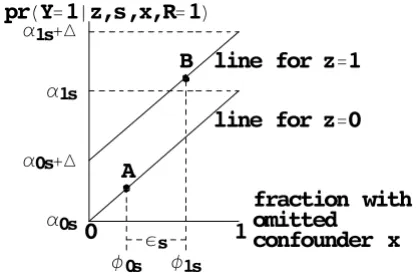
For a tabular display of these calculations see Table 1. For a graphical depiction based on the BK-plot [17,18], see Figure 1.
From (18) the bias from omitting x in stratum s is ψs εs. The first factor
ψs = pr(Y = 1|Z = 0, s, X = 1, R = 1) - pr(Y = 1|Z = 0, s, X = 0, R = 1) (19)
is the effect of X on subjects in the control group with ob-served outcomes. By virtue of the MAR assumption in (9), we could also write ψs = pr(Y = 1|Z = 0, s, X = 1) - pr(Y = 1|Z = 0,5, X = 0), which is the effect of X on all subjects in the control group. The second factor,
εs = pr(X = 1|Z = 1, s, Z = 1) - pr(X = 1|Z = 0, s, R = 1), (20)
ranges from -1 to 1 and measures the degree of confound-ing between X and Z among subjects with observed out-comes (i.e. R = 1). If εs = 0, there is no confounding and pr R z s y pr R z s x pr y z s x pr x s
pr y z s x x
x
=
( )=∑ ( = ) ( ) ( )
∑
1| , , 1| , , | , , |
| , ,
(( ) (pr x s| ) , ( )10
∆apparents
∆ = ( = = = )− ( = = = )
=
= ∑
s
x x
pr Y x Z s R pr Y x Z s R
apparent 1 1 1 1 0 1
0 1 0
1
, | , , | , ,
∑ ∑
∑
∑
= ( = = = ) ( = = = )
− = =
=
=
pr Y Z s R pr X x Z s R
pr Y x Z x
x
0 1
0 1
1 1 1 1 1
1 0
| , | , ,
, | ,, ,s R= pr X x Z| , ,s R
( 1) ( = =1 =1) ( )12
∆apparents
∆sapparent = (α0s+ ∆s)(1−φ1s)+(α1s+ ∆s)φ1s−(α0s(1−φ0s)+α φ1s0s)
== ∆ +s ψ εs s. ( )18
Figure 1
BK-plot of bias from an unobserved binary covariate among subjects not missing outcome. The upper diagonal line is the probability of outcome among subjects not missing outcome in randomization group Z = 1. The lower diagonal line is the probability of outcome among subjects not missing outcome in randomization group group Z = 0. For subjects in group 0, the fraction with X = 1 is φ0s and the probability of outcome is indicated by point A. For subjects in group 1, the fraction with X = 1 is φ1s and the probability of outcome is indicated by point B. The true treatment effect ∆s is the difference between the diagonal lines. The apparent treatment effect ∆s is the vertical distance between points A and B, which equals
∆ + ψsεs, where εs = φ1s - φ0s and ψs = α1s - α0s = the slope of each diagonal line. To bound the overall bias Σsψsεspr(S = s), we specify an upper bound for εs based only on the fraction missing and a plausible value for the maximum of ψs based on the estimates of ψs if an observed covariate were missing.
B
A
Hs
I0s I1s
line for z
0
line for z
1
D1s
D0s
D1s'
D0s'
fraction with
omitted
confounder x
0
1
no bias because the distribution of X among subjects with observed outcomes is the same in the control and study group. If εs = ± 1 there is complete confounding and the bias reaches the maximum value of ± ψs. Taking a weight-ed average over all strata, the overall apparent treatment effect is
and the overall bias is
bias = Σsψs εs ws. (22)
Remarkably it is possible to obtain simple bounds on εs based only on the proportion of subjects who are missing in each randomized group in stratum s. Let
πzs = pr(R = 1|z, s) (23)
denote the proportion of subjects in randomization group
z and stratum s with an observed outcome. As derived in the Appendix See additional file: 1, the maximum εs, which we call the upper bound factor, is
If only 15% of the subjects are missing in each arm ε(max)s is less than .18. If we let ψmax denote the anticipated max-imum value of ψs, then substituting (24) into (22) gives the anticipated maximum bias,
biasmax = ± ψmax Σs ε(max)s ws, (25)
where the anticipated maximum bias under complete confounding, ψmax, is specified by the investigator; the upper bound factor, ε(max)s, is based on the fraction with observed outcomes in stratum s; and ws is the fraction of subjects in stratum s.
Thus the investigator need only specify ψmax. One might argue that if x were a strong unobserved inherited gene, ψmax would be close to 1. However because, "eligible sub-jects had no history of colorectal cancer, surgical resection of adenomas, bowel resection, the polyposis syndrome, or inflammatory bowel disease" [14], it is unlikely that many subjects had an unobserved high-penetrance gene related to the recurrence of adenomas. We therefore believe that unobserved factors that might affect both adenoma recur-rence and missingness could have an effect of similar mag-nitude as observed baseline covariates. Thus to obtain a plausible value for ψmax, we suggest estimating ψs, as defined in (19), based on observed covariates. (See the Re-sults section.) Of course the relationship between ob-served covariates and missingness could differ substantially from the relationship between an unob-served covariate and missingness. Nevertheless, we be-lieve that estimates of ψs from observed covariates are helpful for specifying a realistic value for ψmax.
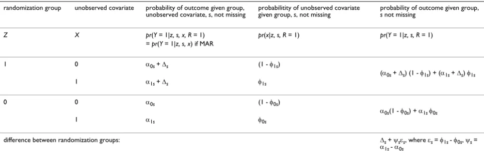
Table 1: Cell probabilities in a generic stratum s
randomization group unobserved covariate probability of outcome given group, unobserved covariate, s, not missing
probabilitity of unobserved covariate given group, s, not missing
probability of outcome given group, s not missing
Z X pr(Y = 1|z, s, x, R = 1) pr(x|z, s, R = 1) pr(Y = 1|z, s, R = 1) = pr(Y = 1|z, s, x) if MAR
1 0 α0s + ∆s (1 - φ1s)
(α0s + ∆s) (1 - φ1s) + (α1s + ∆s) φ1s
1 α1s + ∆s φ1s
0 0 α0s (1 - φ0s)
α0s(1 - φ0s) + α1s φ0s
1 α1s φ0s
difference between randomization groups: ∆s + ψsεs, where εs = φ1s - φ0s, ψs = α1s - α0s
Under missing at random (MAR), the probabilities in the third column are the same for subjects not missing outcome as for all subjects, so ∆s rep-resents the true treatment effect, which is the same for both levels of x. Because the distribution of x is different among subjects not missing out-come in each randomization group, the apparent treatment effect is the difference in weighted averages over x in the last column, namely, ∆s + ψsεs. To bound the overall bias Σsψsεspr (S = s), we specify an upper bound for εs based only on the fraction missing and a plausible value for the maxi-mum of ψs based on the estimates of ψs if an observed covariate were missing.
∆ = ∑ ∆
(
=)
= ∑ ∆ +
(
)
(
=)
= ∆ + ∑
apparent apparent
s s
s s s s
s s s
pr S s pr S s p
ψ ε
ψ ε rr S
(
= s)
,( )
21ε π
π
π π
max s s
s
s os max
( ) = − −
( )
1 1
24 0
1
1
Results
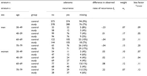
We applied our approach to data from the PPT trial strat-ified by age and sex (Table 2). We first assumed MAR and applied (7) and (8) to estimate the difference in the prob-abilities of adenoma recurrence between the two groups.
We obtained = -.003 with se( ).=.022, which is close to the unstratified estimate and its standard error.
To compute the anticipated maximum bias (25) we first computed ε(max)s using (24) and estimated ws from the observed fractions (Table 2). This gave Σsε(max)s ws = .10. We then specified ψmax, the anticipated maximum bias under complete confounding. To obtain a plausible value for ψmax, we estimated ψs in (19) pretending either sex or
age was the unobserved covariate x. This gave = .23, .18, .18, .19, for the four age categories when x = sex and .07 and .09 for the two sex categories when x = age.
Treat-ing the largest as a realistic lower bound for ψmax, we specified a slightly larger value, ψmax = .25, so that the an-ticipated maximum bias is biasmax = ± .25 × .10 = .025. The
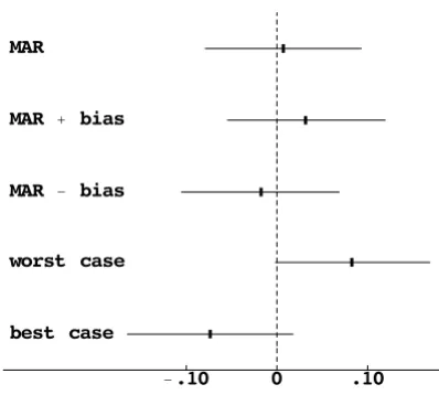
MAR confidence interval is shifted to the right or left by the anticipated maximum bias (Figure 2).
For purpose of comparison, we also computed estimates and confidence intervals under a worst (best) case impu-tation [9,19], where missing outcome data in each stra-tum were imputed as no recurrence (recurrence) in controls and recurrence (no recurrence) in the interven-tion group. (These stratum-specific estimates were com-bined over strata using weights inversely proportional to the stratum-specific variances.) In the worst and best case imputations the confidence intervals did not overlap zero (Figure 2).
Our sensitivity analysis showed that the worst and best case imputations were too extreme. Because the absolute value of the anticipated maximum bias, .025, is smaller
than 1.96 × se ( ) = .043, the bias-adjusted confidence in-tervals overlap zero. Thus the anticipated maximum bias of ± .025 did not change our conclusion of little evidence of an effect of treatment on adenoma recurrence. However it did increase our uncertainty, as the more extreme lower and upper bounds indicated that the true effect of
treat-Table 2: Results of Polyp Prevention Trial
stratum s adenoma difference in observed weight bias factor
ε(max)s
stratum s recurrence rates of recurrence ds ws
sex age group no yes missing
control 573 374 94 (9%) study 578 380 76 (7%)
men 30–49 control 33 22 5 (8%) -.23 .07 .09 study 58 12 3 (4%)
40–59 control 99 76 7 (4%) .01 .17 .05 study 94 76 9 (5%)
60–69 control 122 105 25 (10%) -.04 .23 .11 study 144 105 18 (7%)
70–79 control 65 76 26 (16%) -.04 .13 .20 study 70 71 29 (17%)
women 30–49 control 54 11 3 (4%) .03 .10 .07 study 47 12 4 (6%)
40–59 control 69 24 4 (4%) .02 .11 .04 study 69 27 4 (4%)
60–69 control 77 31 13(11%) .08 .12 .11 study 68 40 5 (4%)
70–79 control 54 29 11(12%) .22 .07 .12 study 28 37 4 (6%)
The overall estimate of the difference in probabilities of recurrence between study and control groups is = Σsdsws = -.003 with a standard error .022. We define ε(max)s = max((1 - π0s)/π1s, (1 - π1s)/π0s), where πzs equals one minus the fraction missing in group z and stratum s. The anticipated
maximum bias is ψmax Σs ε(max)s ws = ± .10 ψmax, where ψmax is the anticipated bias if there were complete confounding of the unobserved covariate and treatment.
∆l
∆l ∆l
ψls
ψls
ment could likely be higher or lower than indicated by the original analysis.
Discussion
The key idea of our method is to incorporate non-MAR missingness by postulating an unobserved binary covari-ate. Although similar in spirit to using an unobserved binary covariate with observational data [20], randomiza-tion adds important extra informarandomiza-tion that can be usefully exploited. Our formulation implies that the probability of missingness depends on both outcome and treatment assignment.
The proposed methods hinges on first selecting the appro-priate baseline covariates. We agree with Myers [21] that if one anticipates missing data, one should collect informa-tion on the baseline covariates related to outcome that might predict missing in outcome. We assumed that with-in a stratum, the effect of treatment did not depend on the unobserved binary covariate. We view this as a main effect and thus a reasonable approximation.
We also agree with Shih [1] that one should collect infor-mation on the cause of missingness. In particular we rec-ommend reporting whether any of the missing outcomes were definitely MAR, for example, due to random techni-cal problems, to accidents, or to leaving the study for rea-sons completely unrelated to the investigation. Suppose that outcome was definitely MAR in a proportion vzs of subjects. Then it is more informative to write vzs as pr(R = 1, not MAR|z, s) + vzs. Because vzs contains no information about the effect of X on missingness, one can replace πzs
by πzs - vzs, which reduces ε(max)s and hence reduces the an-ticipated maximum bias.
Although we applied our methodology to a cross-classifi-cation of categorical covariates, it could also be applied to continuous covariates or a univariate combination of co-variates in a manner analogous to a propensity score [22]. Let u denote a vector of covariates and ez = pr(R = 1|z, u). Following the derivation of propensity scores [22], we can write, pr(R = 1|z, ez) = E(r|z, ez) = E(E(r|z, u)|z, ez) = E(ez|z,
ez) = ez. Therefore pr(R = 1|z, u) = pr(R = 1|z, ez), and thus ez contains the same information for the probability of be-ing observed as u. This calculation justifies using ez to summarize the covariates predicting missingness. To form five strata for randomized group z, we would compute ez for each subject in group z and then divide the distribu-tion of ez into quintiles.
Conclusion
The bias due to an unobserved binary covariate could arise when the probability of missingness depends on both treatment and outcome. Computation of the bias is easy because it equals the maximum anticipated bias un-der complete confounding multiplied by an upper bound factor. The maximum anticipated bias might require some expert input but some lower bound values can be obtained using observed baseline covariate. The upper bound factor is easily computed from the fraction missing in each group. The methodology is particularly useful in the common situation when no more than 15% of the subjects (in excess of those definitely MAR) have missing outcomes, so that the upper bound factor in the bias is less than .18.
Contributions
SGB devised the basic model with the unobserved covari-ate, worked out the unconstrained maximization, and wrote the initial draft of the manuscript. LSF worked out the constrained maximization and provided substantive improvements to the manuscript.
Figure 2
Comparison of missing data adjustments for Polyp Preven-tion Trial. The graph plots the estimated differences in the probability of adenoma recurrence between the intevention and control groups and the 95% confidence intervals. MAR is missing at random within strata. MAR ± bias shifts the MAR confidence interval based on the anticipated maximum bias. Worst and best case imputes missing data to the randomiza-tion group that would give the largest positive and negative effect, respectively.
.10 .10
best case worst case MAR bias MAR bias MAR
Publish with BioMed Central and every scientist can read your work free of charge
"BioMed Central will be the most significant development for disseminating the results of biomedical researc h in our lifetime."
Sir Paul Nurse, Cancer Research UK
Your research papers will be:
available free of charge to the entire biomedical community
peer reviewed and published immediately upon acceptance
cited in PubMed and archived on PubMed Central
yours — you keep the copyright
Submit your manuscript here: BioMedcentral
Additional material
References
1. Shih WJ Problems in dealing with missing data and informa-tive censoring in clinical trials. Current Controlled Trials in Cardio-vascular Medicine 2002, 3:4
2. Hollis S A graphical sensitivity analysis for clinical trials with non-ignorable missing binary outcome. Statistics in Medicine 2002, 21:3823-3834
3. Little RJ and Rubin DB Statistical Analysis with Missing Data. John Wiley & Sons, New York 1987,
4. Baker SG, Rosenberger WF and DerSimonian R Closed-form esti-mates for missing counts in two-way contingency tables. Sta-tistics in Medicine 1992, 11:643-657
5. Molenberghs G, Kenward MG and Goetghebeur E Sensitivity anal-ysis for incomplete contingency tables: the Slovenian plebi-scite case. Applied Statistics 2001, 40:15-29
6. Baker SG and Laird NM Regression analysis for categorical var-iables with outcome subject to nonignorable nonresponse. Journal of the American Statistical Association 1988, 83:62-69
7. Baker SG, Ko C and Graubard BI A sensitivity analysis for non-randomly missing categorical data arising from a national health disability survey. Biostatistics 2003, 4:41-56
8. Wittes J, Lakatos E and Probstfield J Surrogate endpoints in clin-ical trials: cardiovascular diseases. Statistics in Medicine 1989, 8:415-425
9. Proschan MA, McMahon RP, Shih JH, Hunsberger SA, Geller NI, Kn-atterud G and Wittes J Sensitivity analysis using an imputation method for missing binary data in clinical trials. Journal of Sta-tistical Planning and Inference 2001, 96:155-165
10. Vach W and Blettner M Logistic regression with incompletely observed categorical covariates-investigating the sensitivity against violation of the missing at random assumption. Statis-tics in Medicine 1995, 14:1315-1329
11. Matts JP, Launder CA, Nelson ET, Miler C and Dain B The Terry BeirnCommunity Programs for Clinical Research on AIDS. Statistics in Medicine 1997, 16:1943-1954
12. Rotnitzky A and Wypij D A note on the bias of estimators with missing data. Biometrics 1994, 50:1163-1170
13. Scharfstein DO, Rotnitzky A and Robins JM Adjusting for non-ignorable drop-out using semiparametric nonresponse mod-els. Journal of the American Statistical Association 1999, 94:1096-1148 (with discussion)
14. Schatzkin A, Lanza E, Corle D, Lance P, Iber F, Caan B, Shike M, Weissfeld J, Burt R, Cooper MR, Kikendall JW, Cahill J, Freedman L, Marshall J, Schoen RE and Slattery M The Polyp Prevention Trial Study Group. Lack of effect of a low-fat, high-fiber diet on the recurrence of colorectal adenomas New England Journal of Medicine 2000, 342:1149-1155
15. Hutton JL Number need to treat: properties and problems. Journal of the Royal Statistical Society Series A 2000, 163:403-419 16. Horvitz DG and Thompson DJ A generalization of sampling
without replacement from a finite population.Journal of the American Statistical Association 1952, 47:663-685
17. Wainer H The BK-Plot: Making Simpson's paradox clear to the masses. Chance 15:60-62
18. Baker SG and Kramer BS Good for women, good for men, bad for people:Simpson's paradox and the importance of sex-specific analysis in observationalstudies. Journal of Women's Health & Gender-Based Medicine 2001, 10:867-872
19. Horowitz JL and Manski CF Nonparametric analysis of rand-omizedexperiments with missing covariate and outcome
data (with discussion). Journal of the American Statistical Association 2000, 95:77-88
20. Rosenbaum PR and Rubin DB Assessing sensitivity to an unob-served binarycovariate in an observational study with binary outcome. Journal of the RoyalStatistical Society, Series B 1983, 45: 212-218
21. Myers WR Handling missing data in clinical trials: an overview. DrugInformation Journal 2000, 34:525-533
22. Rosenbaum PR and Rubin DB Reducing bias in observational studies using sub-classification on the propensity score. Jour-nal of the American Statistical Association 1984, 79:516-524
Pre-publication history
The pre-publication history for this paper can be accessed here:
http://www.biomedcentral.com/1471-2288/3/8/prepub
Additional file 1
Click here for file