DEMOGRAPHIC RESEARCH
A peer-reviewed, open-access journal of population sciences
DEMOGRAPHIC RESEARCH
VOLUME 36, ARTICLE 34, PAGES 989–1014
PUBLISHED 29 MARCH 2017
http://www.demographic-research.org/Volumes/Vol36/34/ DOI: 10.4054/DemRes.2017.36.34
Research Article
Best-practice life expectancy: An extreme
value approach
Anthony Medford
c
2017 Anthony Medford.
1 Introduction 990
2 Data 992
3 Methods 995
3.1 Motivation 995
3.2 Classical extreme value theory: Basics 996
3.3 The setup 997
3.4 A note on assumptions 999
4 Results 1000
4.1 Fitted models 1000
4.2 Applications 1002
4.2.1 Projections 1002
4.2.2 Probabilities 1003
4.2.3 Other inference 1004
5 Discussion 1004
6 Concluding remarks 1005
7 Acknowledgements 1006
References 1007
Appendix A 1010
Appendix B 1012
Appendix C 1013
Best-practice life expectancy: An extreme value approach
Anthony Medford1
Abstract
BACKGROUND
Whereas the rise in human life expectancy has been extensively studied, the evolution of maximum life expectancies, i.e., the rise in best-practice life expectancy in a group of populations, has not been examined to the same extent. The linear rise in best-practice life expectancy has been reported previously by various authors. Though remarkable, this is simply an empirical observation.
OBJECTIVE
We examine best-practice life expectancy more formally by using extreme value theory.
METHODS
Extreme value distributions are fit to the time series (1900 to 2012) of maximum life expectancies at birth and age 65, for both sexes, using data from the Human Mortality Database and the United Nations.
CONCLUSIONS
Generalized extreme value distributions offer a theoretically justified way to model best-practice life expectancies. Using this framework one can straightforwardly obtain prob-ability estimates of best-practice life expectancy levels or make projections about future maximum life expectancy.
COMMENTS
Our findings may be useful for policymakers and insurance/pension analysts who would like to obtain estimates and probabilities of future maximum life expectancies.
1Max Planck Odense Center on the Biodemography of Aging and University of Southern Denmark. E-Mail:
1. Introduction
Mortality projections are crucial in many areas. In life insurance and pensions where the financial well-being of millions of individuals is at stake, these projections are crucial. Globally, governments and other stakeholders depend on reliable mortality projections for management and administration of their financial liabilities.
Oeppen and Vaupel (2002) introduced the term ‘best-practice life expectancy’ (BPLE), referring to the maximum life expectancy observed among national populations during a particular year. Their best-practice life expectancies at birth have been increas-ing in a nearly linear fashion, beginnincreas-ing in Scandinavia around 1840 and continuincreas-ing ever since at a pace of about 0.24 years per annum for females and 0.22 years per annum for males (Oeppen and Vaupel 2002). In a later study that covered a longer period (1750– 2005) Vallin and Mesl´e (2009) indicated instead that life expectancy increased in a piece-wise linear fashion over four distinct periods. Nonetheless, their basic results, especially for recent decades, are generally consistent with the overall pattern of increase of about three months per year (Vaupel 2012). Additionally, Shkolnikov et al. (2011) showed that best practice cohort female life expectancy at birth increased across cohorts born from 1870 to 1920 by an average of about 0.43 years annually.
There is a strong argument for using life expectancy in forecasting. White (2002) found that linear trends in life expectancy give a better fit to the experience of individual countries than linear trends in age-standardized (log) death rates in his study of 21 devel-oped countries. Among those who have forecast life expectancy are Alho and Spencer (2005), Andreev and Vaupel (2006), Lee (2006), and Torri and Vaupel (2012). Oeppen and Vaupel (2002) argue that since the increase in best-practice life expectancy is linear and regular then it could be used in forecasting by comparing country-specific perfor-mance with the best practice. This approach takes advantage of national mortality trends, which ought to be considered within a larger international context rather than being ana-lyzed and projected individually (Lee 2006).
problems can be tackled. Torri and Vaupel (2012), Andreev and Vaupel (2006), and Lee (2006) proposed methods which attempt to do this.
Although the consistent evolution of BPLE for over a century and a half is remark-able, this is simply an empirical observation; in the original work of Oeppen and Vaupel (2002) no attempt was made to formally model BPLE. Torri and Vaupel (2012) employed classic univariate ARIMA techniques, but their emphasis was on forecasting country-specific life expectancy where they forecast the BPLE and, separately, the gap between the BPLE and country-specific life expectancy. In this paper we propose a formal theo-retical model for BPLE using arguments from extreme value theory (EVT).
Extreme value statistical methodology has previously been used in a mortality de-mographic context. Some of the earliest work using EVT in a dede-mographic application began with Gumbel (1937, 1958). More recently, a number of papers involving the use of EVT have been published. Aarssen and De Haan (1994) estimated a finite upper bound on the distribution of human life spans, contrary to Galambos and Macri (2000), who countered that such an upper bound could not exist. Thatcher (1999) modeled the highest attainable age by using classical EVT. Watts, Dupuis, and Jones (2006) modeled the high-est attained age by using the generalized extreme value (GEV) distribution. Han (2005) uses EVT to model the death rates for the elderly. Li, Hardy, and Tan (2008) use some classical results from EVT to develop a model called the threshold life table in order to extrapolate survival distributions to the oldest ages and to close a life table. Hanayama and Sibuya (2015) estimate the upper limit of the lifetime probability distribution of the Japanese population.
The primary aim of this article is to explore the modeling of best-practice life ex-pectancies by using extreme value theory. Secondarily, we investigate how fitted EVT models may be used to make inferences about future levels of life expectancy. We note that our application of the theory is somewhat different from previous work in that we attempt to fit a model to life expectancy directly, whereas previous work fitted models to high ages at death. Our key contribution is to show that BPLE may be modeled using EVT.
2. Data
The data for use in model implementation and testing comes from two sources. First, the Human Mortality Database (HMD 2015) covers the low-mortality countries that have the best data and the highest life expectancies. It contains life tables for 37 countries plus all the raw data used in constructing these tables. The specific data used was life expectancy at birth and at age 65, for both males and females, and covers the period 1900 to 2012. For a small number of years, some eastern European populations – former Soviet Republics – had the highest life expectancies. Among these are Poland, Lithuania, Belarus, Russia, and Ukraine. These life expectancies were likely to be overstated, so whenever this occurred the second highest value, which appeared more plausible, was taken to be the annual maximum.
The second source of data covers all other countries according to the standard United Nation definitions and classifications as of 6 November 2013 (UN Statistics Division 2013). Life expectancies at birth and age 65 from these countries cover the period 1950– 2012 and amount to a further 204 countries. This data is available from the UN World Population Prospects: The 2015 Revision (United Nations, Department of Economic and Social Affairs, Population Division 2015). In total, there is data from 241 countries.
The following notation will be used throughout:
e∗x: best-practice life expectancy at given agexwhere”∗”indicates maximum e∗x,f: best-practice life expectancy at given agexfor females
e∗x,m: best-practice life expectancy at given agexfor males.
Oeppen and Vaupel (2002) first highlighted the remarkable linearity in the BPLE. Figure 1 presents a plot of these BPLEs, separately for males and females, at birth and age 65, from the year 1900 and identifies which countries were leaders. The (piecewise) linear nature of the BPLEs and how few countries managed to attain best-practice levels of life expectancy are clearly seen.
Figure 1: Countries with the highest life expectancies at birth and age 65, males and females separately, from 1900–2012
1900 1920 1940 1960 1980 2000
50 55 60 65 70 75 80 85
Female best-practice e0
Year e0 * Iceland Japan Norway NZ (non−Maori) Sweden
1900 1920 1940 1960 1980 2000
50 55 60 65 70 75 80 85
Male best-practice e0
Year e0 * Australia Denmark Iceland Japan Netherlands
NZ (non−Maori) Norway Sweden Switzerland
1900 1920 1940 1960 1980 2000
12 14 16 18 20 22 24
Female best-practice e65
Year e65 * Canada France Iceland Japan Norway NZ (non−Maori) Sweden
1900 1920 1940 1960 1980 2000
12 14 16 18 20 22 24
Male best-practice e65
Year e65 * Australia Denmark Iceland Japan Norway Switzerland
is largely due to mortality reductions due to advances in the treatment and prevention of cardiovascular diseases that primarily affect the elderly.
Figure 2: Breakpoints in the trend of the highest life expectancies at birth and age 65, males and females separately, from 1900–2012
1900 1920 1940 1960 1980 2000
50
55
60
65
70
75
80
85
Females
e0
*
1900 1920 1940 1960 1980 2000
50
55
60
65
70
75
80
85
Males
e0
*
1900 1920 1940 1960 1980 2000
12
14
16
18
20
22
24
Females
e65
*
1900 1920 1940 1960 1980 2000
12
14
16
18
20
22
24
Males
e65
3. Methods
3.1 Motivation
Extreme value statistics facilitate the investigation of stochastic processes at very high or very low levels, and extreme value distributions arise as the limiting distributions of the maxima or minima of a set of random variables. In this paper we are interested in studying the evolution of the maximum life expectancies among all countries.
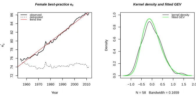
Figure 3 presents the BPLE at birth for females. It is well known that life expectancy has been increasing over time at all ages, and this is evident in a strong upward trend in the time series of the BPLE. The left panel presents this data from 1955 along with another series representing the same data but with the linear least-squares regression trend removed in order to produce a stationary series. The right panel shows a nonparametric estimate of this stationary data (we use the kernel density) and a fitted GEV distribution. The data has also been scaled by subtracting the intercept term of the fitted regression. Graphically, the fitted distribution appears to provide a very reasonable fit to the annual maximum data. Based on this evidence, one can conclude that extreme value theory may be useful in analyzing the BPLE.
Figure 3: Left panel: Raw and detrended data. Right panel: Kernel density and fitted GEV distribution
1960 1970 1980 1990 2000 2010
72
74
76
78
80
82
84
86
Year
e0
*
Female best-practice e0
observed detrended trend line
−1.0 −0.5 0.0 0.5 1.0 1.5 2.0
0.0
0.2
0.4
0.6
0.8
1.0
N = 58 Bandwidth = 0.1659
Density
Kernel density and fitted GEV
3.2 Classical extreme value theory: Basics
In this section we present some basics of the general classical extreme value theory. The specifics for our particular model will be put forward in subsequent sections. The limiting distributions of extremes give rise to the extreme value distributions. In this article, the parameterizations and notation of Coles (2001) will be used.
Formally, suppose thatX1,X2,. . .,Xn is a sequence of independent random vari-ates all having a common distribution functionF(x). Let the maximum of this sequence ofnvariables beMn. We would like to find the distribution ofMnasnbecomes large. Now,
P(Mn ≤z) =P(X1≤z,X2≤z,. . .,Xn≤z) =P(X1≤z)P(X2≤z). . . P(Xn≤z)
=Fn(z).
This result, though, is not particularly useful as the distribution of F(x)is unknown. However, it is possible to find the distribution ofMn (for largen), sayG, without any reference toF.
The distribution ofMn is degenerate because, asntends to infinity, Fn(z) → 0 for anyzless than the upper end point of the support of F. To avoid the difficulty of the degenerate limit, a linear rescaling ofMnis applied – a result known as the extremal types theorem (Fisher and Tippett 1928; Gnedenko 1943; Coles 2001).
If there exist sequences of constants{an>0}and{bn}, such that asn→ ∞, PMn−bn
an
≤z→G(z), (1)
whereG(z)is a nondegenerate distribution function, then Gmust be a member of the generalized extreme value (GEV) family of distributions. This is a striking result because regardless of the underlying distribution, the distribution of the maxima (or minima) con-verges to one of the generalized extreme value family of distributions.
The GEV distribution function is given by
G(z) = expn−h1 +ξ(z−µ
σ )
i−1ξ o
, (2)
The shape parameter,ξ, determines the heaviness of the right tail. This leads to three types of distributions: Whenξ <0, the distribution has finite support and is short-tailed; leading to the Weibull distribution. Whenξ >0, there is polynomial tail decay, leading to heavy tails; the GEV is of the Fr´echet type. The case whereξ= 0is taken to be the limit of Eq. 2 asξ →0and there is exponential tail decay leading to light tails, and the GEV is of the Gumbel type with distribution function
G(z) = expn−exph−(z−µ
σ )
io
.
In practice, for sufficiently large n,G(z)can be calculated without the need to know the normalizing constants {an > 0} and{bn} (Coles 2001). This has motivated an approach to GEV modeling known as the block maxima approach, where for large enough n,P(Mn ≤z)can be approximated by using an appropriate member of the GEV family. Briefly, the block maxima approach works as follows: Suppose we have independent observationsX1,X2,. . .. Let these observations be divided into blocks of lengthnfor
sufficiently largen. Then, take the maximum of each of these blocks to obtain a series of block maxima and fit a GEV distribution to these maxima in order to obtain parameter estimatesµˆ, σˆ, and ξˆ. (See Section 3.3 for details on our approach.) For inference, estimates of extreme quantiles of the maxima are obtained by solving forzpin equation 2:
zp=µ− σ ξ
h
1− {−log(1−p)}−ξi, (3)
where the distribution function of the GEV,G(zp) = 1−pandpis the tail probability or the probability of realizing a value at least as large aszp.
In extreme value terminology, the quantiles of the distribution, zp, are sometimes called return levels and are associated with the so-called return period1/p. If we consider annual maxima, which is usually the case, then on average the quantilezpis expected to be exceeded with probabilitypor on average once every 1/pyears (Coles 2001). For example, ifp= 0.01then the return levelzpis the 99th percentile and corresponds to the
1/(1−0.01) = 100-year return period. It is the amount which one expects to see once
every 100 years, on average.
3.3 The setup
For us, because BPLE is an already defined metric and partly because annual life ex-pectancies are more common and useful in practice, we choose block lengths of one year. Each block represents a sample of sizen = 241period life expectancies,X1,X2,. . .,
X241from each country represented in our dataset. From this sample, we select the
max-imum,Z241. This is done for each yeart= 1. . . tmax, wheretmaxis the last year of the data, resulting in a series of block maximaZ241,t;t= 1. . . tmaxto which a GEV model is fitted.
The linear trend over time ine∗xis accounted for by allowing the location parameter of the GEV model to vary linearly with time such that, instead of a fixed location pa-rameterµ, a more flexible parameter is adopted. Thus, time is introduced as a covariate into the parametrization of the GEV distribution, so we assume a location parameter of the form,µt = µ0+µ1t, wheretrepresents calendar time. More specifically,t is an
index commencing at 1 in the first year of the data (e.g., 1950 fore∗0,f ) and increases by one unit per consecutive year. The parameterµ1could be interpreted as roughly the
annual rate of increase in life expectancy. The parameterµ0is the fitted initial level of
the location parameter for the first year of data. Sincee∗
xhas been trending upward linearly over time,µ, the location parameter of the GEV, is the most obvious parameter of the GEV to capture this feature, but we point out that time dependence could also be introduced into the other parameters, provided that the additional complexity is justified and strongly supported by the data. In general, however, the shape parameter,ξ, is not usually altered as it can be difficult to estimate in practice (Coles 2001). For our model we assume that all the time dependence ine∗xis sufficiently captured by the time-varying location parameter,µt.
Although several methods are available, maximum likelihood estimation (MLE) is often a sensible choice because of its relative flexibility and ability to easily incorporate covariate information (Coles 2001; Coles and Dixon 1999). We propose MLE for finding the parameters of the GEV distributionµ0,µ1,σ, andξ. Denote byz1,. . .,ztmax the sequence of the maxima taken over each data block. Assuming independent maxima, the log likelihood function is defined as
`(µ0,µ1,σ,ξ) =−
tmax X
t=1
logσ+ (1 + 1/ξ) logh1 +ξzt−(µ0+µ1t)
σ
i
+
h
1 +ξzt−(µ0+µ1t)
σ
i−1ξ
!
,
solution; therefore, numerical procedures are used to jointly estimate the value of the parametersµˆ0, ˆµ1, ˆσ, andξˆ, which maximizes the log-likelihood function. Numerical
optimization is done using the R package ‘extRemes’.
3.4 A note on assumptions
We now briefly discuss the key assumptions of the classical GEV model and contrast them with our setup and data realities. It is important to bear in mind that the GEV is based on asymptotics. The classical theory is based on maxima taken from blocks consisting of independent, identically distributed variables. Our model does not assume a stationary distribution of extremes as a separate GEV is assumed for each year, as elaborated previously. Therefore, our discussion is mainly on the issue of dependence betweene∗
x. First, a comment on within-block dependence is in order. Although there may be some common underlying trends in closely connected countries, we consider the overall dependence in life expectancy between the 241 countries within each block to be sufficiently independent as to not compromise the use of the GEV distribution. Life expectancy in, say, Angola would not under normal circumstances be related to that in Sweden, for example.
On the other hand, between blocks – at extremal levels – there exists dependence which we, for expository purposes, categorize loosely as temporal and nontemporal. This is not a rigid distinction, and the effects may not be easy to disentangle in practice. From a temporal perspective, human mortality trends evolve very stably and, barring catastrophes such as war or pandemics, a high period life expectancy should be followed by the same. We also observe that countries tend to achieve the BPLE in clusters; this pattern is most evident amongst females at birth where only eight countries have been the leader since 1840 (Oeppen and Vaupel 2002).
From a nontemporal perspective, the world’s populations are becoming more in-timately connected via transportation, communication, trade, and technology. Wilson (2011) documented the convergence of global mortality levels over recent decades. The low-mortality countries which have held the BPLE are becoming more similar in their lifestyles, and globalization is also acting on practices affecting mortality, contributing to converging mortality patterns (Wilson 2011; White 2002; Edwards and Tuljapurkar 2005). As a consequence, there has been a significant degree of convergence ine0within
our group of low-mortality countries, but less so ine65.
countries in our study more similar in distribution, enhancing the arguments for using the GEV. On the other hand, these same factors affect mortality across all countries, leading to greater dependence amongst the mortality patterns and trajectories.
We concede that mortality convergence may be a feature of our group of low-mortality countries, resulting in dependence between consecutive BPLEs and likely in-troducing some bias into the parameter estimates, thus resulting in underestimation of standard errors. For modeling purposes we make no distinction between whether any de-pendence is temporal or driven by some other underlying mechanism. What we can say with certainty is that the effects of dependence manifest themselves through time. As a result, we assume that any dependence in life expectancies is due to time effects.
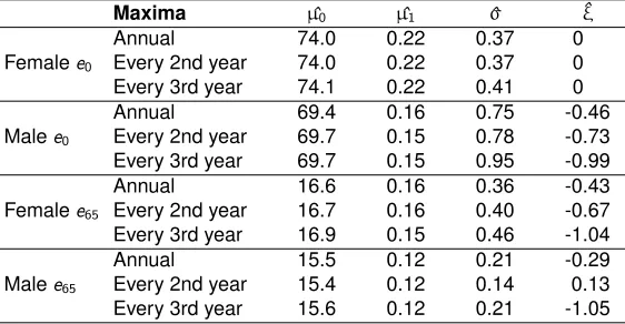
To estimate the magnitude of the impact of any dependence between (e∗x,t,e∗x,t+1) we conduct a simple sensitivity analysis. The parameter estimates for the GEV models are recalculated, but rather than using the full dataset we exclude some annual maxima by using data spaced further apart in time. If temporal dependence is strong, then fitting the model using data spaced further apart should substantially impact the GEV parameter estimates. In other words, if dependence is not substantial, then refitting the model using data spaced further apart should not excessively alter the parameter point estimates, and the change should be within a reasonable order of magnitude. The results of this (see Appendix B) suggest that temporal dependence is not an impediment for fitting the GEV model.
4. Results
4.1 Fitted models
Torri and Vaupel (2012) used data from 1900 to fit BPLE. They argued that this period was used because it is nearly linear, while the longer time series available from 1840 varies in a piecewise linear fashion (Vallin and Mesl´e 2009). However, as demonstrated in Figure 2, there have also been structural breaks during the 20th century; therefore, we do not fit the BPLE arbitrarily from 1900 but from the point of the most recent structural break, which varies depending on the underlying population. By doing this, we ensure that the correct pace of life expectancy increase is attributed to the correct time period and population. Hence, the fitting periods are from 1950 fore∗0,m(representing males at birth), from 1955 fore∗0,f (females at birth), from 1967 fore∗65,f (females at age 65), and from 1984 fore∗65,m(males at age 65).
In summary, we fit time-dependent GEV models:
zt∼GEV(µt,σ,ξ),
isξ, andt = 1. . . tmax, wheretmaxis the last year of the data over which the model is fitted.
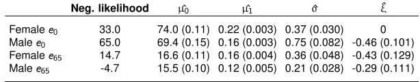
Appendix A presents fitted model diagnostics and shows that the models fit the data well. Using the parameter estimates from Table 1 results in the following fitted GEV models for extreme life expectancy. Note that the shape parameter of the GEV fore∗0,f is zero, indicating a Gumbel distribution. The estimated value for this parameter was about –0.05, but a likelihood ratio test of significance indicated that this value was not significantly different from zero. The negative shape parameters for the others indicate Weibull distributions.
Table 1: Maximized negative log-likelihoods, parameter estimates, and standard errors (in parentheses) of the block maxima model;e0and
e65for males and females shown separately
Neg. likelihood µ^0 µ^1 ^σ ^ξ
Femalee0 33.0 74.0 (0.11) 0.22 (0.003) 0.37 (0.030) 0
Malee0 65.0 69.4 (0.15) 0.16 (0.003) 0.75 (0.082) -0.46 (0.101)
Femalee65 14.7 16.6 (0.11) 0.16 (0.004) 0.36 (0.048) -0.43 (0.129)
Malee65 -4.7 15.5 (0.10) 0.12 (0.005) 0.21 (0.028) -0.29 (0.111)
For female life expectancy at birth: GEV(74.0 + 0.22t, 0.37) For male life expectancy at birth: GEV(69.4 + 0.16t, 0.75,−0.46) For female life expectancy at 65: GEV(16.6 + 0.16t, 0.36,−0.43) For male life expectancy at 65: GEV(15.5 + 0.12t, 0.21,−0.29)
Because EVT is concerned with rare events, it is convenient to make inferences on the extreme quantiles (return levels) of the fitted model. Using Equation 3 and the fitted parameter estimates from Table 1, our time-varying return levels are easily calculated. If we use male life expectancy at birth data, in yeart, the 98th percentile (50-year return level) estimates the highest life expectancy we might expect to encounter on average every 50 years and is given by
z0.02(t) = (69.4 + 0.16t) + 1.62
h
1− {−log(1− 1
50)}
0.46i
.
lines representing the upper quantiles are more spaced out and are closer together for the lower quantiles. The reverse is true for the Weibull. The return levels can also be used in an objective way to identify periods of unusually high or low life expectancy because realizations of high or low life expectancy do not necessarily imply extremities. Suppose that the criteria for extreme life expectancy is a realization higher than the 99th percentile. Then one can immediately identify from Figure 4 the data of interest. Indeed, if the model-fitting period is at least as long as the return period of interest, then it would be possible to compare the theoretical tail probability with the observed. For example, the 98th quantile implies a 2% tail probability or a probability that the quantile would be realized once every 50 years. If the 98th percentile is exceeded regularly, one can assume that mortality experience has been unusually light, leading to the high life expectancy, and investigate further. If we consider the upper 95th percentile from Figure 4 we can make these types of comparisons. Over the period 1955–2012 fore∗0,f we would expect to observe a life expectancy in the upper 5% tail about three times over that 60-year period. In reality we observe four. For an assessment of the predictive performance of the model refer to Appendix D.
4.2 Applications
4.2.1 Projections
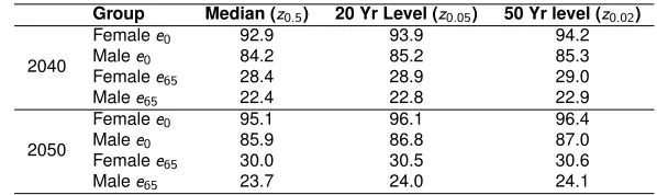
The return levels from Figure 4, similar to the data, evolve in a linear way. If we assume that the current rate of increase ine∗
x continues over a given forecast horizon, then it is possible to project return levels. Table A–1 presents the 100-year, 20-year, and 2-year (median) return levels in 2040 and 2050 (prediction intervals not shown). For example, in 2040, the mediane∗65,mat age 65 is 22.4 years, but the 98th percentile is 22.9 years. Appendix B provides plots of the quantiles for the years 2013 to 2050. A key assumption is that the linear trend forµcontinues beyond the range of data we have observed.
Table 2: Projected extreme life expectancy return levels in 2040 and 2050
Group Median (z0.5) 20 Yr Level (z0.05) 50 Yr level (z0.02)
2040
Femalee0 92.9 93.9 94.2
Malee0 84.2 85.2 85.3
Femalee65 28.4 28.9 29.0
Malee65 22.4 22.8 22.9
2050
Femalee0 95.1 96.1 96.4
Malee0 85.9 86.8 87.0
Femalee65 30.0 30.5 30.6
Figure 4: Best-practice life expectancies and the fitted GEV median, 20-year and 100-year return levels
e0
*
70
75
80
85
1960 1970 1980 1990 2000 2010
median
lower/upper 95th percentile
lower/upper 99th percentile Females
e0
*
70
75
80
85
1950 1960 1970 1980 1990 2000 2010
median
lower/upper 95th percentile lower/upper 99th percentile
Males
e65
*
16
18
20
22
24
1970 1980 1990 2000 2010 median
lower/upper 95th percentile
lower/upper 99th percentile Females
e65
*
16
18
20
22
24
1985 1990 1995 2000 2005 2010
median
lower/upper 95th percentile
lower/upper 99th percentile Males
4.2.2 Probabilities
a one-third chance that by 2025 the maximum observed life expectancy of 65-year-old females will reach 27 years.
Table 3: Probability of the maximum female life expectancies at birth,e∗
0,f,
exceeds certain levels for the years 2020 and 2050
Year P(e0,∗f >90) P(e0,∗m>85) P(e65,∗f >26) P(e65,∗ m>24)
2025 0.23 <0.001 0.57 <0.001
2050 >0.999 0.86 >0.999 0.05
4.2.3 Other inference
Conversely, if we have the life expectancy quantile and assume some level of probability, we can estimate the future time when the given life expectancy level will be observed. For example, if we adopt a significance level of 95%, then maximum female life expectancy at birth observed in the world would reach 100 years around 2070; with 95% probability the country with the highest male life expectancy at age 65 would reach 27 years around 2080.
The foregoing analysis is based on worldwide maxima. The blocks to which the block maxima method was applied contained all countries in the world. However, pro-vided that there is sufficient high-quality life expectancy data available and the underlying assumptions are still valid, the methods of the previous section can be applied to some subregion.
5. Discussion
Sincee∗xis the maximum annual life expectancy at agexfrom among the different na-tions, we have shown that the theory of extreme value statistics can be applied. We used data beginning in 1900, found structural breakpoints, and fit GEV distributions from the most recent breakpoint. This was done in order to ensure that the correct pace of life expectancy improvement was captured for each specific subpopulation.
Projection of the BPLE can be an important component in forecasting life expectancy. According to the work on this method introduced by Oeppen and Vaupel (2002) and fur-ther elaborated by Torri and Vaupel (2012), forecasts of country-specific life expectancy can be obtained by first projecting the BPLE and then modeling and forecasting the gap between the BPLE and the life expectancy in any given population. Torri and Vaupel (2012) used classical univariate time series ARIMA models to forecaste∗0,f ande∗0,m. While this is an obvious and straightforward approach, there are some advantages to our methodology. First, there is the strong theoretical justification for using EVT to fit max-ima data, and second, with our approach it is possible to not only projecte∗xbut also to straightforwardly obtain probabilities about future values ofe∗x.
We calculated the median ofe∗0,f in 2050 to be 95.1 years, which is lower than the 96.59 years found by Torri and Vaupel (2012). Fore∗0,mit is 85.9 years versus 88.38 years in Torri and Vaupel (2012). This is unsurprising, since, as was shown in Section 2, the pace of life expectancy increase for females has slowed to about 0.21 years per year from around 1955, so that the constant drift term of about 0.24 years per year in the ARIMA model overestimates the future value of BPLE. Similarly, for males at birth the pace has slowed to about 0.17 years per year from 1950 versus a constant ARIMA drift of about 0.20 years per year. On the other hand, using the UN projections of life expectancy for all countries, we obtain mediane∗0,fande∗0,min 2050 of 91.35 years (Hong Kong) and 86.2 years (Israel) respectively. Our projection for females is higher. This is because the UN median projection model assumes a much slower pace of increase than ours of around 0.1 years per year. For males, however, our model and the UN’s result in very similar projections of BPLE.
6. Concluding remarks
In this analysis we used extreme value theory to analyze the time series of annual max-imum life expectancy, which to our knowledge has not been previously attempted. We were able to use the fitted model to project future values of BPLE and make probability statements about future values of maximum life expectancy.
turn could be driven by war, disease, or some other catastrophic event that affects life expectancy in an adverse way.
Future work will include the evaluation of robust prediction intervals for any projec-tions. We can also investigate other EVT approaches, such as using more order statistics, where one can model the five highest life expectancies, for example. Models making use of covariates other than time and applied to parameters other than the location parameter could also be explored. Finally, more sophisticated approaches to forecasting the GEV could be explored.
7. Acknowledgements
References
Aarssen, K. and De Haan, L. (1994). On the maximal life span of humans.Mathematical
Population Studies4(4): 259–281.doi:10.1080/08898489409525379.
Alho, J. and Spencer, B.D. (2005). Statistical demography and forecasting. New York: Springer.
Andreev, K.F. and Vaupel, J.W. (2006). Forecasts of cohort mortality after age 50. Max
Planck Institute for Demographic Research Working Paper12.
Coles, S. (2001). An Introduction to statistical modeling of extreme values. New York: Springer. doi:10.1007/978-1-4471-3675-0.
Coles, S.G. and Dixon, M.J. (1999). Likelihood-based inference for extreme value
mod-els. Extremes2(1): 5–23. doi:10.1023/A:1009905222644.
Davies, R. (2002). Hypothesis testing when a nuisance parameter is present only under the alternative: Linear model case. Biometrika 89(2): 484–489.
doi:10.1093/biomet/89.2.484.
Edwards, R.D. and Tuljapurkar, S. (2005). Inequality in life spans and a new perspective on mortality convergence across industrialized countries.Population and Development
Review31(4): 645–674. doi:10.1111/j.1728-4457.2005.00092.x.
Fisher, R.A. and Tippett, L.H.C. (1928). Limiting forms of the frequency distribution of the largest or smallest member of a sample. Mathematical Proceedings of the
Cam-bridge Philosophical Society24(2): 180–190. doi:10.1017/S0305004100015681.
Galambos, J. and Macri, N. (2000). The life length of humans does not have a limit.
Journal of Applied Statistical Science9(4): 253–264.
Gnedenko, B. (1943). Sur la distribution limite du terme maximum d’une s´erie al´eatoire.
Annals of Mathematics44(3): 423–453.doi:10.2307/1968974.
Gumbel, E. (1958).Statistics of extremes. New York: Columbia University Press.
Gumbel, E.J. (1937). La dur´ee extrˆeme de la vie humaine. Paris: Hermann et cie.
Han, Z.J. (2005). Living to 100 and beyond: An extreme value study. In: Johansen, R.J. (ed.).Living to 100 and Beyond Symposium Monograph.
Hanayama, N. and Sibuya, M. (2015). Estimating the upper limit of lifetime probability distribution, based on data of Japanese centenarians. The Journals of Gerontology
Series A: Biological Sciences and Medical Sciences:glv113.
Huerta, G. and Sans´o, B. (2007). Time-varying models for extreme values.Environmental
Human Mortality Database. University of California, Berkeley (USA), and Max Planck Institute for Demographic Research (Germany). (Available at http://www.mortality.org.). Data downloaded on feb. 2, 2015.
Lee, R. (2006). Perspectives on mortality forecasting. III. The linear rise in life ex-pectancy: History and prospects. Stockholm: Swedish Social Insurance Agency: 19– 44.
Li, J.S.H., Hardy, M.R., and Tan, K.S. (2008). Threshold life tables and their applications. North American Actuarial Journal 12(2): 99–115.
doi:10.1080/10920277.2008.10597505.
Oeppen, J. and Vaupel, J.W. (2002). Broken limits to life expectancy.Science296(5570): 1029–1031.doi:10.1126/science.1069675.
ˇSevˇc´ıkov´a, H., Li, N., Kantorov´a, V., Gerland, P., and Raftery, A.E. (2016). Age-specific mortality and fertility rates for probabilistic population projections. In: Schoen, R. (ed.). Dynamic Demographic Analysis. New York: Springer: 285–310.
doi:10.1007/978-3-319-26603-915.
Shkolnikov, V.M., Jdanov, D.A., Andreev, E.M., and Vaupel, J.W. (2011). Steep increase in best-practice cohort life expectancy. Population and Development Review37(3): 419–434.doi:10.1111/j.1728-4457.2011.00428.x.
Thatcher, A.R. (1999). The long-term pattern of adult mortality and the highest attained
age. Journal of the Royal Statistical Society: Series A (Statistics in Society)162(1):
5–43.doi:10.1111/1467-985X.00119.
Torri, T. and Vaupel, J.W. (2012). Forecasting life expectancy in an in-ternational context. International Journal of Forecasting 28(2): 519–531.
doi:10.1016/j.ijforecast.2011.01.009.
United Nations, Department of Economic and Social Affairs, Population Divi-sion (2015). World Population Prospects: The 2015 Revision. Tech. rep., United Nations, Department of Economic and Social Affairs, Population Division. https://esa.un.org/unpd/wpp/Download/Standard/Population.
United Nations Statistics Division (2013). Countries or areas, codes and abbreviations [electronic resource]. http://unstats.un.org/unsd/methods/m49/m49alpha.htm.
Vallin, J. and Mesl´e, F. (2009). The segmented trend line of highest life expectan-cies. Population and Development Review 35(1): 159–187.
doi:10.1111/j.1728-4457.2009.00264.x.
Watts, K.A., Dupuis, D.J., and Jones, B.L. (2006). An extreme value analysis of advanced age mortality data. North American Actuarial Journal 10(4): 162–178.
doi:10.1080/10920277.2006.10597419.
White, K.M. (2002). Longevity advances in high-income countries, 1955–96.Population
and Development Review28(1): 59–76. doi:10.1111/j.1728-4457.2002.00059.x.
Wilmoth, J.R. (1998). Is the pace of Japanese mortality decline converging to-ward international trends? Population and Development Review 24(3): 593–600.
doi:10.2307/2808156.
Wilson, C. (2011). Understanding global demographic convergence since 1950.
Population and Development Review 37(2): 375–388.
Appendix A: Diagnostic tests
0.0 0.2 0.4 0.6 0.8 1.0
0.0
0.2
0.4
0.6
0.8
1.0
empirical
model
Residual probability plot
−1 0 1 2 3 4
−1
0
1
2
3
4
empirical
model
Residual quantile plot (Gumbel scale)
0.0 0.2 0.4 0.6 0.8 1.0
0.0
0.2
0.4
0.6
0.8
1.0
empirical
model
Residual probability plot
−1 0 1 2 3 4
−1
0
1
2
3
4
5
empirical
model
0.0 0.2 0.4 0.6 0.8 1.0
0.2
0.4
0.6
0.8
1.0
empirical
model
Residual probability plot
−1 0 1 2 3 4
−1
0
1
2
3
4
5
empirical
model
Residual quantile plot (Gumbel scale)
0.0 0.2 0.4 0.6 0.8 1.0
0.0
0.2
0.4
0.6
0.8
1.0
empirical
model
Residual probability plot
−1 0 1 2 3
−1
0
1
2
3
4
5
empirical
model
Appendix B: Parameter sensitivity tests for temporal dependence
Table A–1: Sensitivity tests of GEV parameter estimates using data spaced further apart in time. Estimates ofµ^0are rounded to one
decimal place; all other parameter estimates are rounded to two decimal places
Maxima µ^0 µ^1 ^σ ^ξ
Femalee0
Annual 74.0 0.22 0.37 0
Every 2nd year 74.0 0.22 0.37 0
Every 3rd year 74.1 0.22 0.41 0
Malee0
Annual 69.4 0.16 0.75 -0.46
Every 2nd year 69.7 0.15 0.78 -0.73
Every 3rd year 69.7 0.15 0.95 -0.99
Femalee65
Annual 16.6 0.16 0.36 -0.43
Every 2nd year 16.7 0.16 0.40 -0.67
Every 3rd year 16.9 0.15 0.46 -1.04
Malee65
Annual 15.5 0.12 0.21 -0.29
Every 2nd year 15.4 0.12 0.14 0.13
Every 3rd year 15.6 0.12 0.21 -1.05
The estimated parameter values for the different populations in general are not greatly affected by using data spaced farther apart. The parameter ξˆis the key parameter of interest in this sensitivity analysis as it determines the shape of the distribution and, hence, the parametric family to which the fitted model belongs. By using data further apart, we look for two things: first, that the change in parameter values due to the re-estimation is not disproportionately large and, second, that there be no change in the distributional family on account of the re-estimated shape parameter. These criteria are met in all cases except for the malee65population. We attribute this to unreliable parameter estimates
Appendix C: Projected quantiles
e0 * 75 80 85 90 951960 1980 2000 2020 2040 median
10-year level (90th percentile) 20 - year level (95th percentile) 50-year level (98th percentile) 100-year level (99th percentile)
Females e0 * 70 75 80 85
1960 1980 2000 2020 2040
median
10-year level (90th percentile) 20-year level (95th percentile) 50-year level (98th percentile) 100-year level (99th percentile)
Males e65 * 18 20 22 24 26 28 30
1980 2000 2020 2040 median
10-year level (90th percentile) 20-year level (95th percentile) 50-year level (98th percentile) 100-year level (99th percentile)
Females e65 * 16 18 20 22 24
1990 2000 2010 2020 2030 2040 2050
median
10-year level (90th percentile) 20-year level (95th percentile) 50-year level (98th percentile) 100-year level (99th percentile)
Appendix D: Predictive performance
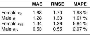
We initially considered comparing the quantiles from the fitted model to sample quantiles but decided against it as the model quantiles would generally be higher than actuals, plus many of the life expectancies calculated for less developed regions are themselves crude approximations.
As a rough check we comparezˆ0.1(ti)to max[ex(ti+ 1),. . .,ex(ti+ 10)]fort=
1985,. . ., 2002andx= 0, 65. We fit the model using data up to 1984 (the most recent
structural breakpoint of the four subpopulations). Because the 10-year return level is attained, on average, once every 10 years, we compare return levels calculated each year with the rolling maxima observed over successive forward-looking 10-year periods. Only data up to 2002 could be used due to the 10-year forecast, which precluded any longer return periods being used.
The evaluation is done using the standard forecast accuracy measures: mean abso-lute error (MAE), root mean squared error (RMSE), and mean absoabso-lute percentage error (MAPE). The forecasting performance appears reasonable, with an average error between about 2% for femalee0and 5.84% for femalee65.
Table A–2: Predictive assessment of fitted models
MAE RMSE MAPE
Femalee0 1.68 1.70 1.98 %
Malee0 1.28 1.33 1.61 %
Femalee65 1.34 1.36 5.84 %