A new automatic method for estimating the peak auroral emission height from all-sky camera images

(1)

Geosci. Instrum. Method. Data Syst., 2, 131–144, 2013 www.geosci-instrum-method-data-syst.net/2/131/2013/ doi:10.5194/gi-2-131-2013

EGU Journal Logos (RGB)

Advances in

Geosciences

Open Access

Natural Hazards

and Earth System

Sciences

Open Access

Annales

Geophysicae

Open Access

Nonlinear Processes

in Geophysics

Open Access

Atmospheric

Chemistry

and Physics

Open Access

Atmospheric

Chemistry

and Physics

Open Access Discussions

Atmospheric

Measurement

Techniques

Open Access

Atmospheric

Measurement

Techniques

Biogeosciences

Open Access Open Access

Biogeosciences

Discussions

Climate

of the Past

Climate

of the Past

Discussions

Earth System

Dynamics

Earth System

Dynamics

Discussions

Geoscientific

Instrumentation

Methods and

Data Systems

Open Access

_{Geoscientific}

Instrumentation

Methods and

Data Systems

Geoscientific

Model Development

Geoscientific

Model Development

Discussions

Hydrology and

Earth System

Sciences

Open Access

Hydrology and

Earth System

Sciences

Ocean Science

Discussions

Solid Earth

Discussions

The Cryosphere

Discussions

Natural Hazards

and Earth System

Sciences

Open Access

Discussions

A new automatic method for estimating the peak

auroral emission height from all-sky camera images

D. K. Whiter1, B. Gustavsson2,*, N. Partamies1, and L. Sangalli3

1_{Finnish Meteorological Institute, Helsinki, Finland}

2_{School of Physics and Astronomy, University of Southampton, Southampton, UK} 3_{Royal Military College of Canada, Kingston, Ontario, Canada}

*_{now at: EISCAT Scientific Association, Kiruna, Sweden}

Correspondence to: D. K. Whiter ([email protected])

Received: 4 September 2012 – Published in Geosci. Instrum. Method. Data Syst. Discuss.: 25 October 2012 Revised: 14 February 2013 – Accepted: 15 February 2013 – Published: 7 March 2013

Abstract. This paper presents a new fully automatic method for quickly finding the average peak emission height of a sin-gle auroral structure from a pair of all-sky camera images with overlapping fields of view. The peak emission height of the aurora must be estimated in order to calculate sev-eral other important parameters, such as horizontal spatial scales, optical flow velocities, and ionospheric electric fields. In most cases the height is not measured, but a value is as-sumed, often about 110 km. It is unclear how accurate this assumption is. A future statistical study of the auroral height in which the method presented here will be applied to many years of observations will lead to more accurate assumptions of the height with quantitative error estimates, and there-fore more accurate estimates of parameters derived using these assumed auroral heights. In the present work the perfor-mance of the new method is compared to another recent au-tomatic method. It is found that the new method measures the peak emission height regardless of the shape of the volume emission rate profile, unlike the other recent method. How-ever, the new method is less suitable than the other method for analysis of very wide auroral arcs (>30 km) or for aurora in the magnetic zenith of one of the images.

1 Introduction

An estimate of the height of maximum auroral emission is often needed for the derivation of other parameters, such as the widths of auroral structures, optical flow velocities, iono-spheric electric field estimates, and electron precipitation

en-ergies (e.g. Kaila, 1989; Knudsen et al., 2001; Whiter et al., 2008; Dahlgren et al., 2009; Partamies et al., 2010; Obuchi et al., 2011). However, the height of the aurora is rarely mea-sured; often when a numerical value is required it is assumed, typically at about 110–130 km for the most prominant emis-sion at 557.7 nm. The accuracy of these assumptions is generally not well known.

This paper presents a new automated method for deter-mining the peak emission height of the aurora from a pair of simultaneous all-sky camera images with partially overlap-ping fields of view. The motivation for this work is to develop a method suitable for performing a large statistical study of the height of the aurora in which hundreds of thousands of images will be analysed. Such a statistical study is expected to substantially improve estimates of the height under differ-ent conditions and the uncertainty introduced by assuming a value for the height in the derivation of other parameters. The peak emission height of the aurora depends on the energy of electron precipitation producing the aurora and the concen-tration profiles of the major neutral species in the thermo-sphere (e.g. Rees, 1963b; Judge, 1972). Long-term change and periodicity in these parameters could be identified using such a large statistical study of the height of the aurora.

(2)

132 D. K. Whiter et al.: Automatic method for estimating auroral emission height

automatic (for single arcs) and require no manual input dur-ing the analysis. It is desirable that the method used in the statistical study can successfully analyse all possible shapes and types of aurora. The present work examines the accuracy of the methods when analysing a variety of shapes and sizes of a single auroral structure located between two stations.

2 Instrumentation

The MIRACLE (Magnetometers – Ionospheric Radars – All-sky Cameras Large Experiment) network includes sev-eral (between 5 and 8, depending on year) all-sky cam-eras distributed across northern Fenno-Scandinavia and Sval-bard (Syrjäsuo et al., 1998) with overlapping fields of view. The all-sky cameras have been in continuous winter opera-tion since 1996, and have produced many thousands of im-ages of the aurora (∼105 images per station per season), making them particularly suited for a statistical study into the height of the aurora. In this work three of the cam-eras, stationed at Abisko (68.36◦N, 18.82◦E), Kilpisjärvi (69.01◦N, 20.79◦E) and Sodankylä (67.42◦N, 26.39◦E), have been used. Initially the MIRACLE cameras used in-tensified charge-coupled device (ICCD) detectors, but these were upgraded to a mixture of colour CCDs and electron-multiplying CCD (EMCCD) detectors in 2006 and 2007. In this work only ICCD data are used, but data from the EM-CCD observations will also contribute to the future statistical study.

The ICCD and later EMCCD all-sky cameras are each equipped with a filter wheel and set of narrow passband (∼2 nm) interference filters for observing auroral emis-sion at 630.0 nm (“red”), 557.7 nm (“green”), and 427.8 nm (“blue”), together with panchromatic images. The filter wheels attached to the EMCCD cameras also include filters for observing background emission. Only green images have been used in this work, but it is expected that the statistical study will involve all filters. The imaging sequence can be modified but is synchronised across all MIRACLE stations such that all cameras are observing in the same wavelength at the same time. Generally the cameras have produced a green image at least once per 20 s and blue and red images at least once per minute. The exposure time of the ICCD images has usually been 1 s for green and panchromatic images and 2 s for blue and red images.

3 Previous work

Sangalli et al. (2011) used a manual triangulation method to find the peak emission height of an auroral arc observed with the same all-sky cameras as are used in the present work. They found the peak emission height of the arc varied by about 40 km along its length, and the mean height varied be-tween 120±10 km and 140±10 km over a period of 6 min. Although the method they used gives information about the

variation in height along auroral arcs, it is not ideal for a large-scale statistical study as it is time consuming and re-quires considerable manual input, prompting the develop-ment of the new method presented here. The new method does not give information about the variation in height along an arc, but is fast and automated.

Several workers developed methods to identify the height of the aurora during the 1960s. Naturally these methods were applied manually, although some could now be automated to take advantage of modern computers. However, modern computers allow the application of other methods (such as the new method presented here) which would have been pro-hibitively time consuming in the 1960s.

Roach et al. (1960) used a triangulation method to find the height of exceptional “monochromatic” red aurora at low latitude using three all-sky cameras. They found a peak emis-sion height of 412±23 km. The method relies on the as-sumption that the auroral arc lies along parallels of equal magnetic dip angle, which is valid for the exceptional red arcs but renders the method unsuitable for a statistical study in the Arctic. Rees (1963a) developed a method for deter-mining the height of similar auroral forms to Roach et al. (1960) from a single all-sky camera image. The main disad-vantage of this method is that it only works for arcs which are exactly east–west aligned. This assumption is most valid for arcs at relatively low latitude (for which this method was developed) with heights well above 100 km, and is therefore not suitable for application to the MIRACLE data or for a statistical study.

A method for determining the height of aurora, which in-volves measuring the parallax between corresponding im-ages from a pair of simultaneous wide-angle (nearly all-sky) cameras, was used by Brandy and Hill (1964). This method relies on accurately identifying the lower border of a well-defined arc, and gives the height of this lower border rather than the height of peak emission. Similar parallactic pho-tography methods were used many years earlier with nar-rower field-of-view cameras (e.g. St¨ormer, 1955; Harang, 1951; McEwen and Montalbetti, 1958). Boyd et al. (1971) discussed the reasons for measuring the peak emission height rather than the height of the lower border of the arc. The peak emission height is more closely related to the energy of the precipitating electrons than the height of the lower border of the arc (Rees, 1963b). Also, the location of the lower bor-der is dependent on the sensitivity of the observing instru-ment, and therefore combining measurements from different instruments can produce incorrect results for the height of the aurora, especially if the instruments are of different ages. The new method presented in this work is designed to mea-sure the height of peak emission, and so does not suffer from these problems.

(3)

D. K. Whiter et al.: Automatic method for estimating auroral emission height 133

Disussion

P

ap

er

|

Disussion

P

ap

er

|

Disussion

P

ap

er

|

Disussion

P

ap

er

|

−2500 −200 −150 −100 −50 0 50 50

100 150

S₁ S₂

Height (km)

−250 −200 −150 −100 −50 0 50

S₁

Distance North (km) S₂

−250 −200 −150 −100 −50 0 50

S₁ S₂

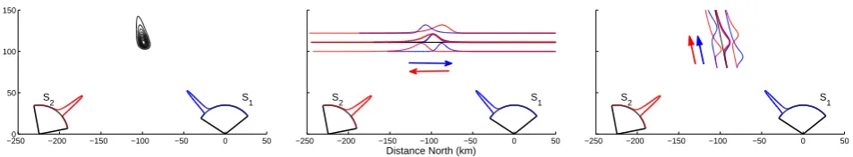
Fig. 1. Cartoon showing the projection of images of an auroral arc located between two stations

(shown in left panel) on to three different horizontal planes (middle panel) and three different

geomagnetic field lines (right panel). The colour-coded arrows in the middle and right panels

indicate the “up” direction in each projection. This shows that in the case of the horizontal plane

the shape of the two projections is flipped.

H.: Small-scale structures in flickering aurora, Geophys. Res. Lett., 35, L23 103, doi:10.1029/

2008GL036134, 2008.

625

24

Fig. 1. Cartoon showing the projection of images of an auroral arc located between two stations (shown in left panel) onto three different

horizontal planes (middle panel) and three different geomagnetic field lines (right panel). The colour-coded arrows in the middle and right panels indicate the “up” direction in each projection. This shows that in the case of the horizontal plane the shape of the two projections is flipped.

geomagnetic meridian. They produced a mathematical for-mulation for synthetic auroral arcs as viewed by MSPs, and tested the triangulation method for different arc positions, widths, and height profiles. They found that the method over-estimated the height when the arc was located between the two stations, and underestimated the height for arcs which were far away from both stations, but worked well when the arc was overhead one of the two stations. They also sug-gested an iterative technique to determine volume emission rate profiles of quiet auroral arcs using this method, which was used in a second paper (Romick and Belon, 1967b).

Boyd et al. (1971) used the triangulation method tested by Romick and Belon (1967a) for identifying the peak auroral emission height from a system of three meridian scanning photometers located on the same dipole meridian. The scan-ning photometer instrumentation restricts their study to quiet and homogeneous structures. Other workers also used this technique, but applied to two photometers only (e.g. Sand-holt et al., 1982; Sigernes et al., 1996; Deehr et al., 2005). Sigernes et al. (1996) emphasise that their analysis is re-stricted to narrow auroral structures. Jackel et al. (2003) ar-gued that a good angular resolution is required for this tech-nique, as the resulting height measurement is sensitive to er-rors in the angle of the intensity peak. Instead they developed a technique in which scans from a pair of meridian scanning photometers are projected onto an invariant latitude grid at a range of assumed heights. The height which produces the largest correlation coefficient between the two scans is taken as the peak emission height. Ashrafi et al. (2005) expanded the method to 2-dimensional camera images. A fast and au-tomatic version of this method is evaluated in this work, and is described fully in Sect. 4.1 below.

Tomographic-like inversion is another technique which has recently been used for finding the height of atmospheric emission from camera images (e.g. Frey et al., 1996; Aso et al., 1998; Gustavsson, 2000; Tanaka et al., 2011). How-ever, this method is not ideal for a statistical study as it re-quires too time-consuming computations and manual input to preprocess the images. Also, to be accurate it requires images of the same structure observed from many stations, which is not often possible due to varying local weather

con-ditions and cloud cover at the different stations. This would therefore reduce the size of a statistical study.

With the exception of the method used by Ashrafi et al. (2005), none of the above methods are suitable for a sta-tistical study using all-sky cameras either because they are not fully applicable to the instrumentation, they are too time-consuming, or they are not sufficiently accurate when applied to a range of different auroral structures (including measur-ing the lower border of the arc rather than the peak emission height).

4 Methods and analysis

The two methods used in this work to determine the auroral peak emission height both involve projecting or “remapping” overlapping images from a pair of stations and maximising the correlation between the remapped images. The main dif-ference between the two methods is the type of remapping. Method 1 is a version of the method used by Ashrafi et al. (2005) in which images are mapped onto a horizontal plane. The second method is novel and has not been previously used to estimate the height of atmospheric emission. In this new method images are mapped onto the Earth’s magnetic field lines.

4.1 Method 1: horizontal plane

(4)

134 D. K. Whiter et al.: Automatic method for estimating auroral emission heightDisussion

P

ap

er

|

Disussion

P

ap

er

|

Disussion

P

ap

er

|

Disussion

P

ap

er

|

Fig. 2. Synthetic images of the same arc for all-sky cameras in a) Kilpisj ¨arvi and b) Sodankyl ¨a.

A single geomagnetic field line is highlighted in cyan.

25

Fig. 2. Synthetic images of the same arc for all-sky cameras in (a) Kilpisj¨arvi and (b) Sodankyl¨a. A single geomagnetic field line

is highlighted in cyan.

The method is illustrated in the middle panel of the 2-dimensional illustration shown in Fig. 1. Images of an au-roral arc observed by two stations, S1 (blue) and S2 (red),

are shown projected onto a horizontal plane at three different heights. On the central plane the images (red and blue bright-ness curves) are most highly correlated, and so the height of this plane is taken as the peak emission height of the aurora. Figure 1 is explained in more detail later in this paper. 4.2 Method 2: magnetic field lines

In this method the all-sky camera images are projected onto individual magnetic field-lines rather than a horizontal plane. The basic concept behind this is illustrated in Fig. 2, which shows synthetic images of a single thin auroral arc

viewed simultaneously by the Kilpisjärvi (a) and Sodankylä (b) MIRACLE stations. The method for generating these syn-thetic images is described later in Sect. 5. Projecting a 2-dimensional image onto a single field-line is equivalent to taking a curved cut across the image. In Fig. 2, one geomag-netic field line is marked in cyan in the altitude range 80– 200 km. One end of the cut corresponds to the bottom of the field line (80 km altitude), while the other end of the cut cor-responds to the top (200 km altitude). The same field line is highlighted in the images from Kilpisjärvi and Sodankylä.

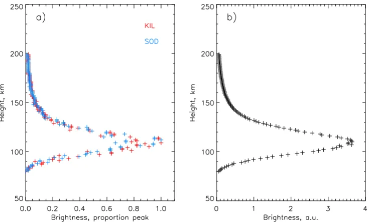
When an image of an arc is projected onto a field line whose geographic position (latitude and longitude) coincides with that of the arc, the field line cut across the image can be used to extract an emission height profile for the arc at that location. Figure 3a shows the emission altitude profile ex-tracted from the Kilpisj¨arvi (red) and Sodankyl¨a (blue) im-ages for the field line marked in Fig. 2. The field line lays within the simulated arc, and the profiles from the two cam-eras correlate well (correlation coefficient 0.99). It is likely that the two profiles would not correlate well if the field line was outside the arc. Method 2 examines many field lines at different locations and uses three tests (described below) to identify which field lines lay within (or very close to) the au-roral structure. Figure 3b shows the emission altitude profile for the whole arc, created by averaging together the altitude profiles for all field lines which passed the three tests. The peak height is found to be 110 km, which is equal to the true peak height of the synthetic arc.

The different outcomes for “good” field lines located very close to an auroral structure and those located further away are illustrated in the right panel of Fig. 1, simplified in 2 di-mensions. The images of the arc from S1(blue) and S2(red)

are shown projected onto three different field lines at differ-ent locations. On the cdiffer-entral field line the two projections are very similar and highly correlated. Projecting the images onto the other two field lines shown in the illustration do not lead to profiles which are highly correlated, and therefore these profiles would not pass the three tests and would not be included in the mean volume emission rate profile for the auroral structure.

(5)

P

ap

er

|

Disussion

P

ap

er

|

Disussion

P

ap

er

|

Disussion

P

ap

er

|

Fig. 3. a) Altitude profile extracted from the field line highlighted in figure 2a for Kilpisj ¨arvi (red) and Sodankyl ¨a (blue). b) Average over all field lines which pass the three tests. The brightness is shown in arbitrary units (a.u.).

26

Fig. 3. (a) Altitude profile extracted from the field line highlighted in Fig. 2 for Kilpisj¨arvi (red) and Sodankyl¨a (blue). (b) Average over all

field lines which pass the three tests. The brightness is shown in arbitrary units (a.u.).

uniform distribution with a mean spacing of 0.05◦in latitude and 0.075◦in longitude at 100 km altitude (∼5 km separa-tion). The positions are random because it was found that if they conformed to a regular grid, the result could be biased to either lower or higher altitudes if the arc lay approximately parallel, but slightly away from, one row of the grid. A se-lection of 10 random field line footprints are marked with coloured crosses in the top panels of Fig. 4. The field lines at each point are traced between 80 km and 200 km altitude using the 10th generation International Geomagnetic Refer-ence Field (IGRF-10) model (Maus et al., 2005). The images are projected onto each of these field lines individually, such that each field line corresponds to a curved cut across each image, as shown in the middle panels of Fig. 4. Those field lines which successfully pass three specific tests are aver-aged together to produce a mean emission altitude profile for the structure. The height of peak emission is taken from this mean altitude profile. The three tests are as follows:

1. The correlation coefficient between the projections from the two images must be greater than 0.5.

2. The field line must show a clear peak in the brightness altitude profile (peak brightness substantially higher than the means of both the upper and lower portions of the field line. The required peak to mean ratio varies depending on the overall brightness of the structure, in order to work with different types of image).

3. The seperation between the luminosity height profile averages (analogous to centre of mass) of the two pro-jections must be smaller than 20 km.

After analysis under these conditions, a second iteration is performed in which the mean spacing between field lines is reduced by a factor 3 and only the regions surrounding field lines which “passed” the first iteration are considered. For this second iteration the tests are made more stringent; the correlation coefficient must be greater than 0.7 and the spread between the luminosity height profile averages must be smaller than 1 km. The analysis is performed over 2 itera-tions in this way to reduce the computational time required. The bottom panels of Fig. 4 show the altitude profiles ex-tracted from the dark blue (left) and dark red (right) field line cuts. The profiles from the Kilpisjärvi and Sodankylä images are shown as solid and dashed lines, respectively. The bright-ness scale is arbitrary. The horizontal black lines mark the luminosity height profile averages. In the case of the dark blue field line (left panel), the luminosity height profile av-erages of the Kilpisjärvi (solid) and Sodankylä (dashed) pro-files are close, and the field line passes the tests for inclusion in the average profile. However, in the case of the dark red field line (right panel), the separation between the luminosity height profile averages is quite large, and so this field line is rejected in the second iteration.

5 Synthetic images

(6)

Disussion

P

ap

er

|

Disussion

P

ap

er

|

Disussion

P

ap

er

|

Disussion

P

ap

er

|

Fig. 4. The testing of different magnetic field lines as part of method 2. Ten selected field lines are shown on synthetic images from the Kilpisj ¨arvi and Sodankyl ¨a stations. Top: the footprints of the test field lines at 100 km height. Middle: the projections of the field lines as cuts on the images. Bottom: height profiles for a “successful” test field line (dark blue, left), and a “failed” test field line (dark red, right).

₂₇

Fig. 4. The testing of different magnetic field lines as part of method

2. Ten selected field lines are shown on synthetic images from the Kilpisj¨arvi and Sodankyl¨a stations. Top: the footprints of the test field lines at 100 km height. Middle: the projections of the field lines as cuts on the images. Bottom: height profiles for a “successful” test field line (dark blue, left), and a “failed” test field line (dark red, right).

each method can be evaluated as the emission height profile of the simulated arcs is known.

The process of generating a pair of synthetic images is illustrated in Fig. 5. Firstly, a rectangular grid of regularly spaced auroral ray “footprints” is generated, as shown in Fig. 5a. These footprints are defined with an arbitrary alti-tude of 100 km, in a N–S/E–W cartesian coordinate system (hence the curvature of the grid when plotted in the latitude– longitude coordinate system of Fig. 5a). Each footprint is 2.5 km from each of its neighbours. The length (450 km) and width (10 km) of the grid of ray footprints defines the length and width of the resulting simulated arc. The loca-tions of the Sodankyl¨a and Kilpisj¨arvi observing staloca-tions are marked in Fig. 5 with blue and red points respectively. Cur-vature is added to the grid of footprints (Fig. 5b) to more accurately represent a real arc, according to a “bendiness” parameter (described below). Next, the grid of footprints is rotated (Fig. 5c) before each footprint is shifted a small

ran-Disussion

P

ap

er

|

Disussion

P

ap

er

|

Disussion

P

ap

er

|

Disussion

P

ap

er

|

Fig. 5. The process for generating synthetic images. a) Initial grid of ray footprints. The red and blue points mark the locations of Kilpisj ärvi and Sodankyl ä respectively. b) Grid of footprints after applying curvature. c) After rotation. d) After adding “noise”. e) The resulting arc as viewed from Sodankyl ä. f) The resulting arc as viewed from Kilpisj ärvi.

28

Fig. 5. The process for generating synthetic images. (a) Initial grid

of ray footprints. The red and blue points mark the locations of Kilpisj¨arvi and Sodankyl¨a respectively. (b) Grid of footprints af-ter applying curvature. (c) Afaf-ter rotation. (d) Afaf-ter adding “noise”.

(e) The resulting arc as viewed from Sodankyl¨a. (f) The resulting

arc as viewed from Kilpisj¨arvi.

dom distance in a random direction to add noise to the grid (Fig. 5d). The final step is to apply the estimated emission al-titude profile shown in Fig. 6 to each auroral ray footprint and to map the emission to the image plane of each camera. The magnetic field line passing through each footprint at 100 km is traced using the IGRF-10 model (Maus et al., 2005) to esti-mate the 3-dimensional shape of the auroral rays. The emis-sion height profile shown in Fig. 6 was created by scaling an atomic oxygen concentration profile from the MSISE-90 model (Hedin, 1991) so that the peak concentration (emis-sion) is at exactly 110 km. Example synthetic images are shown in Fig. 5e and f for the Sodankyl¨a and Kilpisj¨arvi sta-tions, respectively, generated from the footprints shown in Fig. 5d.

(7)

P

ap

er

|

Disussion

P

ap

er

|

Disussion

P

ap

er

|

Disussion

P

ap

er

|

Fig. 6. Volume emission rate profile with a peak at 110 km, used when generating the synthetic images.

29

Fig. 6. Volume emission rate profile with a peak at 110 km, used

when generating the synthetic images.

width ranges from 5 km to 35 km in steps of 5 km. The an-gle ranges from 0◦ _{(east–west aligned) to 90}◦ _{(north–south}

aligned) in steps of 5◦_{(clockwise looking down). The}

bendi-ness ranges from 0.05 to 0.25 in steps of 0.05. The curve of the arc is made up of a combination of sinusoidal and poly-nomial components designed to produce a variety of shapes while accurately representing an auroral arc. The sinusoidal and polynomial components are functions of the bendiness parameter as well as random values. Therefore the bendiness parameter cannot reproduce an exact arc shape, but controls how straight the arc is, with a value of zero corresponding to a perfectly straight arc. Examples of two arcs with different bendiness parameters are shown in Fig. 7. This figure approx-imately illustrates the extremes of curvature of the synthetic arcs used in this study, although it should be noted that as the shape of the arc has some dependence on random val-ues, it is probable that both straighter and more curved arcs form part of the set. Figure 7a and 7b show the location of the ray footprints for simulated arcs with bendiness 0.05 and 0.25, respectively. Figure 7c and d show these two arcs as viewed from Sodankyl¨a. In both cases the arcs are 450 km long, 10 km wide, and have an angle of 10◦with respect to a circle of latitude.

The range of auroral arc lengths within the set of synthetic images (50–700 km) provides an accurate representation of

Disussion

P

ap

er

|

Disussion

P

ap

er

|

Disussion

P

ap

er

|

Disussion

P

ap

er

|

Fig. 7. a) Ray footprints for a simulated arc with bendiness 0.05. b) Ray footprints for a

simu-lated arc with bendiness 0.25. Panels c) and d) show the arcs in panels a) and b) respectively, as viewed from Sodankyl ¨a.

30

Fig. 7. (a) Ray footprints for a simulated arc with bendiness 0.05. (b) Ray footprints for a simulated arc with bendiness 0.25.

Pan-els (c) and (d) show the arcs in panPan-els (a) and (b) respectively, as viewed from Sodankyl¨a.

(8)

P

ap

er

|

Disussion

P

ap

er

|

Disussion

P

ap

er

|

Disussion

P

ap

er

|

Fig. 8. Histograms showing the results from applying method 1 (a) and method 2 (b) to the set of synthetic images. Standard deviations: a) 1.3, b) 4.8.

31

Fig. 8. Histograms showing the results from applying method 1 (a) and method 2 (b) to the set of synthetic images. Standard deviations: (a) 1.3, (b) 4.8.

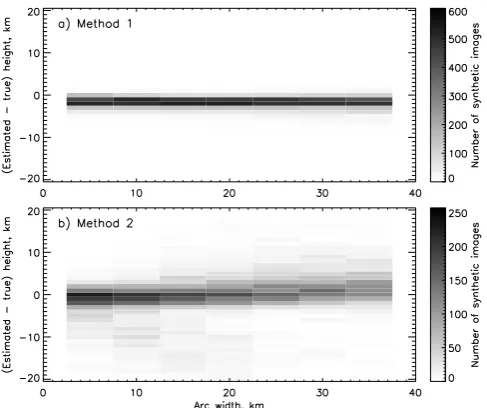
6 Results and discussion

The two methods described in Sect. 4 have been evaluated using the set of synthetic images described in Sect. 5. The height produced by the two methods has been compared to the true peak height of the synthetic arcs, which is fixed at 110 km. Figures 8a and b shows histograms of the differ-ence between the found height and the true height for meth-ods 1 and 2 respectively. The narrow distribution in Fig. 8a (standard deviation = 1.3 km) shows that the horizontal plane method gives a consistent result. However, the peak of the distribution has an offset of−2 km showing that, on average, the method underestimates the peak emission height. In con-trast the distribution for method 2 (Fig. 8b) is considerably wider (standard deviation = 4.8 km), but has its peak at zero height offset, showing that on average the magnetic field-line method produces the correct answer, but the uncertainty is larger than for method 1.

The most probable cause of the 2 km offset in the results from method 1 is that an auroral structure located between the two stations will be projected onto the horizontal plane such that one image will be a mirror image of the other. This can cause the correlation coefficient to be at maximum for a horizontal plane which is not at the height of peak emis-sion. This problem does not occur when projecting onto mag-netic field lines as in method 2, which allows the two pro-jections to be aligned. This concept is illustrated in Fig. 1. The left panel shows a cartoon of an auroral arc (black) lo-cated between two cameras (s1 and s2). The blue and red

curves above the cameras’ fields of view indicate the bright-ness of the arc as observed by s1 and s2 respectively. The

middle panel shows these two brightness curves projected

onto a horizontal plane at three different heights, including the peak volume emission height of the auroral arc (middle projection), as for method 1. The arrows indicate the “up” direction from each projection. It is clear that the shape of each brightness profile is flipped horizontally with respect to the other profile. The right panel of the figure shows the two brightness curves instead projected onto three different mag-netic field lines, as in method 2. In this case the two profiles are aligned, and are most highly correlated when the peaks are at the same height, as for the central field line projection in the right panel of Fig. 1.

(9)

P

ap

er

|

Disussion

P

ap

er

|

Disussion

P

ap

er

|

Disussion

P

ap

er

|

Fig. 9. Histograms showing the distribution of arc angles for images which produce results further than 1 standard deviation from the mean result for a) method 1 and b) method 2.

32

Fig. 9. Histograms showing the distribution of arc angles for images which produce results further than 1 standard deviation from the mean

result for (a) method 1 and (b) method 2.

Disussion

P

ap

er

|

Disussion

P

ap

er

|

Disussion

P

ap

er

|

Disussion

P

ap

er

|

Fig. 10. As figure 8 but showing results from only N-S and E-W aligned arcs for a) method 1 b) method 2. Standard deviations: a) 0.7, b) 2.9.

33

Fig. 10. As Fig. 8 but showing results from only N–S and E–W aligned arcs for (a) method 1 (b) method 2. Standard deviations: (a) 0.7, (b) 2.9.

not lay on the baseline between the two stations and there-fore do not have a large ambiguity between height and length along the arc.

The width of an auroral arc has a substantial effect on the ambiguity between the vertical and horizontal dimen-sions within the 2-dimensional images of the arc. In this work the two methods have been tested using simulated arcs with widths ranging from 5 km to 35 km, as described in Sect. 5. Figure 11 shows how the performance of (a) method 1 and (b) method 2 varies with arc width. Each panel shows seven histograms, one for each arc width tested. The shaded bins

are coloured according to the number of image pairs (the scale on the right of the figure). It is clear from panel (a) that method 1 performs consistently regardless of arc width up to the tested limit of 35 km. The histograms show an al-most constant bias (estimated height – true height) of about

(10)

Disussion

P

ap

er

|

Disussion

P

ap

er

|

Disussion

P

ap

er

|

Disussion

P

ap

er

|

Fig. 11.The effect of the auroral arc width on the performance of a) method 1 and b) method 2.

34

Fig. 11. The effect of the auroral arc width on the performance of (a) method 1 and (b) method 2.

is−2.4 km. Method 1 implicitly assumes that the aurora is predominantly flat and horizontal, whereas method 2 implic-itly assumes that the aurora is made up of rays parallel to the magnetic field. It is therefore logical that method 1 performs well when the aurora is significantly horizontal (such as for 35 km wide arcs) and method 2 performs well when the au-rora is predominantly vertical (such as for thin arcs).

Method 2 involves taking an average profile over multi-ple field lines, each of which can provide an estimate of the peak emission height. The standard deviation of the height over these field lines is related to the accuracy of the method, and to the actual variation in height across the auroral struc-ture. Figure 12 shows the relationship between this standard deviation and the difference between the estimated and true heights for the set of 9310 synthetic images described above as a 2-dimensional histogram. The shaded bins are coloured according to the scale on the right of the figure. The red dashed line highlights where the standard deviation is equal to the difference between estimated and true height. For the majority of test images, this difference is less than the stan-dard deviation (85 % of images, histogram bins below the red dotted line), showing that the standard deviation across “good” test field lines can provide a useful estimate of the uncertainty of the method result. When examining real im-ages, it is important to note that a large standard deviation could result from an auroral structure which does not have one constant peak emission height.

To check that the methods respond to the peak emission height (rather than another property such as mean emission height), synthetic images of the same auroral arc were gen-erated using five different volume emission rate profiles and were analysed using both methods. For each profile the foot-prints of the auroral rays used to generate the synthetic

im-Disussion

P

ap

er

|

Disussion

P

ap

er

|

Disussion

P

ap

er

|

Disussion

P

ap

er

|

Fig. 12.Two dimensional histogram showing the relationship between the standard deviation

of the peak height over all field lines which contribute to the average emission profile in method 2 and the difference between the true peak height and the height estimated by the method.

35

Fig. 12. Two dimensional histogram showing the relationship

be-tween the standard deviation of the peak height over all field lines which contribute to the average emission profile in method 2 and the difference between the true peak height and the height estimated by the method.

ages were identical, and formed an east–west aligned arc 350 km long, 10 km wide and with a bendiness of 0.1. All of the profiles have a peak emission height of 110 km, but each has a different mean emission height. The five profiles are shown in Fig. 13. The results from the two methods are shown on the right of the figure as diamonds, colour-coded to match the height profiles to which they correspond. The same results are shown in the magnified panel (far right) for clarity, where the standard deviations over “good” test field lines used in method 2 (as discussed above) are plotted as error bars with a total length of twice the standard deviation. Both methods respond quite well to the peak emission height for all profiles, but method 2 is clearly less susceptible to variations in the shape of the profile and produces the best results. For all profiles the peak emission height is within the error estimate for method 2. The dark blue-coloured profile was used in the generation of the 9310 synthetic image pairs described in Sect. 5. For this profile method 1 underestimates the peak emission height, which is consistent with the results discussed earlier, but for most other profiles it produces an overestimate.

(11)

D. K. Whiter et al.: Automatic method for estimating auroral emission heightDisussion 141

P

ap

er

|

Disussion

P

ap

er

|

Disussion

P

ap

er

|

Disussion

P

ap

er

|

Fig. 13.Five different volume emission rate profiles used to test whether the methods respond

to the peak emission height. The results from both methods are shown on the right of this figure.

36

Fig. 13. Five different volume emission rate profiles used to test

whether the methods respond to the peak emission height. The re-sults from both methods are shown on the right of this figure.

same ranges as described in Sect. 5. All of the synthetic arcs were approximately east–west aligned. The results of these tests show that method 1 performs consistently for all arc lo-cations which have been tested. However, while method 2 is successful for arcs located approximately halfway between the two stations, it does not perform well for arcs located a few tenths of a degree to the south of either station. In these cases the arc is in the magnetic zenith as viewed from one of the stations, and therefore many auroral rays appear as dots or very short lines in the corresponding image. It is not possi-ble to extract accurate emission profiles from test field lines close to the magnetic zenith, and so method 2 fails to pro-vide a result or performs poorly in these cases. The results of method 2 appear to be biased for arcs located directly above the Kilpisj¨arvi station, but the reason for this is unclear. It is possible that the arcs are so close to the horizon of the So-dankyl¨a images that the pixel resolution is too low to produce reliable altitude profiles from test field lines. It is not possible to analyse arcs located far to the north or south of both sta-tions, as the separation of the stations is too large. The tests performed here are not exhaustive, and further analysis is re-quired to fully assess the performance of the methods for ex-treme arc locations. However, in most cases images suitable for analysis will contain arcs located between the stations.

In addition to analysis of the set of synthetic images, the methods have been trialed on a short set of real images of 557.7 nm emission acquired by the Abisko and Kilpisjärvi cameras. Abisko is approximately 110 km south-west of Kilpisjärvi. Examples from this image set, which displays a single quiet arc, are shown in Fig. 15. The top panel shows an image from Abisko, and the bottom panel shows the coin-cident image from Kilpisjärvi. Although this is only a single short event it is suitable as a simple initial test for the meth-ods presented in this paper as the arc is stable, approximately east–west aligned, and there are no other auroral structures in

Disussion

P

ap

er

|

Disussion

P

ap

er

|

Disussion

P

ap

er

|

Disussion

P

ap

er

|

Fig. 14. Results from the analysis of synthetic arcs located north or south of the midpoint between the Sodankyl ¨a and Kilpisj ¨arvi stations. The same images were analysed using both methods, and results are shown as histograms for a) method 1 and b) method 2.

37

Fig. 14. Results from the analysis of synthetic arcs located north or

south of the midpoint between the Sodankyl¨a and Kilpisj¨arvi sta-tions. The same images were analysed using both methods, and re-sults are shown as histograms for (a) method 1 and (b) method 2.

(12)

142 D. K. Whiter et al.: Automatic method for estimating auroral emission heightDisussion

P

ap

er

|

Disussion

P

ap

er

|

Disussion

P

ap

er

|

Disussion

P

ap

er

|

Fig. 15. Images acquired simultaneously by all-sky cameras in Abisko (top) and Kilpisj ¨arvi

(bottom). Both images show the same auroral arc.

38

Fig. 15. Images acquired simultaneously by all-sky cameras in

Abisko (top) and Kilpisj¨arvi (bottom). Both images show the same auroral arc.

therefore no result was obtained. At these times the results using method 1 are unreliable. In order to avoid such unreli-able results, a test could be applied to images before analy-sis to ensure they contain aurora with a sufficient brightness. Available machine vision methods would be able to perform this test with an accuracy greater than 90 %, although this is not a trivial process (Syrj¨asuo and Partamies, 2011).

The clustering process used in method 2 to select a region of the image for analysis could bias the results, as it restricts

Disussion

P

ap

er

|

Disussion

P

ap

er

|

Disussion

P

ap

er

|

Disussion

P

ap

er

|

Fig. 16. The peak emission height of an auroral arc on 22 November 2000 found using method

1 (black), method 2 (green) and by the manual method of Sangalli et al. (2011) (red). In all cases the Abisko and Kilpisj ¨arvi stations were used.

39

Fig. 16. The peak emission height of an auroral arc on 22

Novem-ber 2000 found using method 1 (black), method 2 (green) and by the manual method of Sangalli et al. (2011) (red). In all cases the Abisko and Kilpisj¨arvi stations were used.

the analysis to a bright structure within the image. It may be expected that the peak emission height of the aurora is related to its brightness (although this is not yet clear). However, this bias will only become apparent for images with aurora cov-ering a very large portion of the image, for example diffuse aurora or a system of many parallel arcs. Under these con-ditions it is likely that the method would fail anyway, as the ambiguity between the horizontal and vertical dimensions in-herent to a 2-dimensional image would be large. It is also unlikely that method 1 would produce a strong correlation between images in these cases.

7 Conclusions

This paper presents a new method for finding the peak emis-sion height of the aurora using simultaneous all-sky camera images from a pair of stations. This method has been devel-oped and tested to evaluate its suitability for a statistical study into the height of the aurora using hundreds of thousands of all-sky camera images from northern Finland. For a statis-tical study of this magnitude, it is vitally important to have a fast and reliable analysis method which is fully automatic. Another method (horizontal plane) has also been tested in the same way as the new method.

(13)

methods are perfect, but both are a marked improvement on earlier methods when considering speed, accuracy and level of automation.

For typical arcs located between the two stations, the field line method (method 2) is recommended, as it responds well to the peak emission height and produces the correct answer on average. It also provides a useful uncertainty estimate. For arcs which are located close to the horizon or in the magnetic zenith of one of the images, the horizontal plane method (method 1) is recommended. This method is also rec-ommended for very wide arcs or aurora which could be con-sidered as predominantly flat (parallel to the Earth’s surface) rather than parallel to the magnetic field. The new field line method is most apropriate for a statistical study of quiet arcs over Lapland, but either method would provide valuable new information on the peak height under different conditions for a large enough data set.

Future work will investigate the possibilty of utilising si-multaneous observations from several (more than two) MIR-ACLE stations to ensure accurate results from arcs with any orientation or location. It may also be possible to apply a combination of the two methods to obtain greater accuracy than either method alone could provide. A hybrid method could also give information about the shape of the volume emission rate profile, as the results of method 1 and method 2 are influenced by the profile shape in different ways. This would require extensive testing. The synthetic images used here contain only a single arc located between the two sta-tions with a constant peak emission height, whereas in reality all-sky camera images often contain multiple auroral struc-tures. Therefore, the methods should be tested on more com-plex synthetic images and synthetic arcs with varying peak emission height. More tests should also be performed on real images for which the peak emission height can be determined using other more precise methods or instruments.

Acknowledgements. This work was financially supported by the

Academy of Finland (grant number 128553). The MIRACLE network is operated as an international collaboration under the leadership of the Finnish Meteorological Institute. The authors thank the participants of the 38th Annual European Meeting on Atmospheric Studies by Optical Methods (38am) for useful comments and suggestions.

Edited by: A. Benedetto

References

Ashrafi, M., Kosch, M. J., and Kaila, K.: Height triangulation of artificial optical emissions in the F-layer, in: Proceedings of the 31st Annual European Meeting on Atmospheric Studies by Op-tical Methods, and 1st International Riometer Workshop, 22– 28 August 2004, Ambleside, UK, 8–16, http://spears.lancs.ac.uk/ publications/31am proceedings.pdf, 2005.

Aso, T., Ejiri, M., Urashima, A., Miyaoka, H., Steen, A.,˚

Br¨andstr¨om, U., and Gustavsson, B.: First results of auroral to-mography from ALIS-Japan multi-station observations in March, 1995, Earth, Planet. Space, 50, 81–86, 1998.

Boyd, J. S., Belon, A. E., and Romick, G. J.: Latitude and Time Variations in Precipitated Electron Energy Inferred from Mea-surements of Auroral Heights, J. Geophys. Res., 76, 7694–7700, 1971.

Brandy, J. H. and Hill, J. E.: Rapid Determination of Auroral Heights, Can. J. Phys., 42, 1813–1819, doi:10.1139/p64-165, 1964.

Dahlgren, H., Ivchenko, N., Lanchester, B., Ashrafi, M., Whiter, D., Marklund, G., and Sullivan, J.: First direct optical observations of plasma flows using afterglow of O+in discrete aurora, J. Atmos. Sol. Terr. Phys., 71, 228–238, doi:10.1016/j.jastp.2008.11.015, 2009.

Deehr, C. S., Rees, M. H., Belon, A. E. H., Romick, G. J., and Lummerzheim, D.: Influence of the ionosphere on the al-titude of discrete auroral arcs, Ann. Geophys., 23, 759–766, doi:10.5194/angeo-23-759-2005, 2005.

Frey, S., Frey, H. U., Carr, D. J., Bauer, O. H., and Haerendel, G.: Auroral emission profiles extracted from three-dimensionally re-constructed arcs, J. Geophys. Res., 101, 21731–21741, 1996. Gustavsson, B.: Three Dimensional Imaging of Aurora and

Air-glow, PhD, Swedish Institute of Space Physics (IRF), Kiruna, Sweden, http://www.irf.se/∼_{bjorn/thesis/thesis.html, (IRF Sci.}

Report 267), ISBN: 91-7191-878-7, 2000.

Harang, L.: The Aurorae, Chapman & Hall, London, 1951. Hedin, A. E.: Extension of the MSIS thermosphere model into the

middle and lower atmosphere, J. Geophys. Res., 96, 1159–1172, doi:10.1029/90JA02125, 1991.

Jackel, B. J., Creutzberg, F., Donovan, E. F., and Cogger, L. L.: Triangulation of Auroral Red-Line Emission Heights, in: Pro-ceedings of the 28th Annual European Meeting on Atmospheric Studies by Optical Methods, 19–24 August 2001, Oulu, Fin-land, edited by: Kaila, K. U., Jussila, J. R. T., and Holma, H., no. 92 in Sodankyl¨a Geophysical Observatory Publications, 97– 100, 2003.

Judge, R. J. R.: Electron Excitation and Auroral Emission Parame-ters, Planet. Space Sci., 20, 2081–2092, 1972.

Kaila, K. U.: Determination of the energy of auroral electrons by the measurements of the emission ratio and altitude of aurorae, Planet. Space Sci., 37, 341–349, 1989.

Knudsen, D. J., Donovan, E. F., Cogger, L. L., Jackel, B., and Shaw, W. D.: Width and structure of mesoscale optical auroral arcs, Geophys. Res. Lett., 28, 705–708, 2001.

Maus, S., Macmillan, S., Chernova, T., Choi, S., Dater, D., Golovkov, V., Lesur, V., Lowes, F., L¨uhr, H., Mai, W., McLean, S., Olsen, N., Rother, M., Sabaka, T., Thomson, A., and Zvereva, T.: The 10th-Generation International Geomagnetic Reference Field, Geophys. J. Int., 161, 561–565, doi:10.1111/j.1365-246X.2005.02641.x, 2005.

McEwen, D. J. and Montalbetti, R.: Parallactic Measurements on Aurorae over Churchill, Canada, Can. J. Phys., 36, 1593–1600, doi:10.1139/p58-161, 1958.

(14)

A00K07, doi:10.1029/2010JA016321, 2011.

Partamies, N., Syrj¨asuo, M., Donovan, E., Connors, M., Charrois, D., Knudsen, D., and Kryzanowsky, Z.: Observations of the au-roral width spectrum at kilometre-scale size, Ann. Geophys., 28, 711–718, doi:10.5194/angeo-28-711-2010, 2010.

Rees, M. H.: A Method for Determining the Height and Geograph-ical Position of an Auroral Arc from One Observing Station, J. Geophys. Res., 68, 175–183, 1963a.

Rees, M. H.: Auroral Ionization and Excitation by Incident Ener-getic Electrons, Planet. Space Sci., 11, 1209–1218, 1963b. Roach, F. E., Moore, J. G., Bruner Jr., E. C., Cronin, H., and

Silver-man, S. M.: The Height of Maximum Luminosity in an Auroral Arc, J. Geophys. Res., 65, 3575–3580, 1960.

Romick, G. J. and Belon, A. E.: The Spatial Variation of Auroral Luminosity–I. The Behavior of Synthetic Model Auroras, Planet. Space Sci., 15, 475–493, 1967a.

Romick, G. J. and Belon, A. E.: The Spatial Variation of Auroral Luminosity–II. Determination of Volume Emission Rate Profiles, Planet. Space Sci., 15, 1695–1716, 1967b.

Sandholt, P.-E., Egeland, A., Henriksen, K., Smith, R., and Sweeney, P.: Optical Measurements of a Nightside Poleward Ex-panding Aurora, J. Atmos. Terr. Phys., 44, 71–79, 1982. Sangalli, L., Gustavsson, B., Partamies, N., and Kauristie, K.:

Esti-mating the Peak Auroral Emission Altitude from All-sky Images, ´

Optica Pura y Aplicada, 44, 593–598, 2011.

Semeter, J., Zettergren, M., Diaz, M., and Mende, S.: Wave dispersion and the discrete aurora: New constraints derived from high-speed imagery, J. Geophys. Res., 113, A12208, doi:10.1029/2008JA013122, 2008.

Sigernes, F., Moen, J., Lorentzen, D. A., Deehr, C. S., Smith, R., Øieroset, M., Lybekk, B., and Holtet, J.: SCIFER-Height mea-surements of the midmorning aurora, Geophys. Res. Lett., 23, 1889–1892, 1996.

St¨ormer, C.: The Polar Aurora, The Clarendon Press, Oxford, 1955. Syrj¨asuo, M. T. and Donovan, E. F.: Using Relevance Feedback in Retrieving Auroral Images, in: Proceedings of the Fourth IASTED International Conference on Computational Intelli-gence, Calgary, Canada, 4–6 July, edited by: Hamza, M. H., 420– 425, IASTED/ACTA Press, 2005.

Syrj¨asuo, M. and Partamies, N.: Numeric Image Features for Detec-tion of Aurora, Geosci. Remote Sens. Lett., IEEE, 9, 176–179, doi:10.1109/LGRS.2011.2163616, 2011.

Syrj¨asuo, M., Pulkkinen, T. I., Janhunen, P., Viljanen, A., Pelli-nen, R. J., Kauristie, K., Opgenoorth, H. J., Wallman, S., Egli-tis, P., Karlsson, P., Amm, O., Nielsen, E., and Thomas, C.: Observations of Substorm Electrodynamics Using the MIRA-CLE Network, in: Proceedings of the International Conference on Substorms-4, Lake Hamana, Japan, 9–13 March, edited by: Kokubun, S. and Kamide, Y., 111–114, Terra Scientific Publish-ing, Tokyo, Japan, 1998.

Tanaka, Y.-M., Aso, T., Gustavsson, B., Tanabe, K., Ogawa, Y., Kadokura, A., Miyaoka, H., Sergienko, T., Br¨andstr¨om, U., and Sandahl, I.: Feasibility study on Generalized-Aurora Computed Tomography, Ann. Geophys., 29, 551–562, doi:10.5194/angeo-29-551-2011, 2011.