https://doi.org/10.5194/gmd-11-5003-2018 © Author(s) 2018. This work is distributed under the Creative Commons Attribution 4.0 License.
The GRISLI ice sheet model (version 2.0): calibration and
validation for multi-millennial changes of the Antarctic ice sheet
Aurélien Quiquet1, Christophe Dumas1, Catherine Ritz2, Vincent Peyaud2, and Didier M. Roche1,3
1Laboratoire des Sciences du Climat et de l’Environnement, LSCE/IPSL, CEA-CNRS-UVSQ, Université Paris-Saclay
Gif-sur-Yvette, France
2Université Grenoble Alpes, CNRS, IRD, IGE, Grenoble, France
3Earth and Climate Cluster, Faculty of Science, Vrije Universiteit Amsterdam, Amsterdam, the Netherlands
Correspondence:Aurélien Quiquet ([email protected]) Received: 16 April 2018 – Discussion started: 2 May 2018
Revised: 23 November 2018 – Accepted: 27 November 2018 – Published: 7 December 2018
Abstract. In this paper, we present the GRISLI (Grenoble ice sheet and land ice) model in its newest revision (version 2.0). Whilst GRISLI is applicable to any given ice sheet, we focus here on the Antarctic ice sheet because it highlights the importance of grounding line dynamics. Important im-provements have been implemented in the model since its original version (Ritz et al., 2001). Notably, GRISLI now in-cludes a basal hydrology model and an explicit flux com-putation at the grounding line based on the analytical for-mulations of Schoof (2007) or Tsai et al. (2015). We per-form a full calibration of the model based on an ensemble of 300 simulations sampling mechanical parameter space us-ing a Latin hypercube method. Performance of individual members is assessed relative to the deviation from present-day observed Antarctic ice thickness. To assess the ability of the model to simulate grounding line migration, we also present glacial–interglacial ice sheet changes throughout the last 400 kyr using the best ensemble members taking advan-tage of the capacity of the model to perform multi-millennial long-term integrations. To achieve this goal, we construct a simple climatic perturbation of present-day climate forc-ing fields based on two climate proxies: atmospheric and oceanic. The model is able to reproduce expected grounding line advances during glacial periods and subsequent retreats during terminations with reasonable glacial–interglacial ice volume changes.
1 Introduction
Addition-ally, glacial troughs may form a deepening bedrock from the grounding line towards the ice sheet centre. Such bed proper-ties lead to the marine ice sheet instability (MISI; Weertman, 1974; Schoof, 2007) responsible for an irreversible retreat of the grounding line in response to an initial perturbation such as local sea level change and/or increase in basal melting rate below ice shelves. The latter two processes are expected to play a crucial role for the stability of the Antarctic ice sheet in the future (e.g. Favier et al., 2014). Additional instabilities may also occur on neutral/prograde bed slopes in relation to structural instabilities of tall ice cliffs (marine ice cliff insta-bility, MICI; Pollard et al., 2015).
Continental ice sheets are difficult to model because they include processes operating on a variety of temporal, from di-urnal to multi-millennial, and spatial scales, from a few me-tres to thousand of kilomeme-tres, but also because we lack cru-cial observations (e.g. basal conditions and internal thermo-mechanics). Most numerical models consider ice sheets as an incompressible fluid, where motion can be described with the Navier–Stokes equations. Even if some processes gener-ally have to be parameterised (e.g. ice anisotropy), the com-plete set of equations can be solved explicitly and does not re-quire the use of any approximation. The most comprehensive continental ice sheet models, namely the full Stokes mod-els, solve explicitly all the terms in the stress tensor (Gillet-Chaulet et al., 2012; Larour et al., 2012). Recent applications are promising but, due to computational cost, continental-scale applications are currently limited to a few centuries. As such, they are not yet the most suitable tool for palaeo-reconstructions or multi-millennial future projections.
In order to decrease the degree of complexity, simpler models were historically developed that make use of the small aspect ratio of ice sheets (vertical- to horizontal-scale ratio) to derive approximations for the Navier–Stokes equa-tions (e.g. Hindmarsh, 2004). Such models are computa-tionally much cheaper than full Stokes models, allowing for multi-millennial integrations. They are well suited to study slow feedbacks such as glacio-isostasy or the impact of tem-perature and surface mass balance perturbations. The Greno-ble ice sheet and land ice (GRISLI) model is one of these simpler models (Ritz et al., 2001). GRISLI consists of the combination of the inland ice model of Ritz (1992) and Ritz et al. (1997) and the ice shelf model of Rommelaere and Ritz (1996), extended to the case of ice streams treated as “drag-ging ice shelves”. In the late 1990s, GRISLI was the first large-scale ice sheet model with a hybrid shallow ice/shallow shelf system of equations. Whilst since Ritz et al. (2001), the fundamental equations for ice dynamics have not drastically changed, the model has nonetheless benefited from numer-ous contributions. To date, 30 papers that have been pub-lished or are in peer review discuss GRISLI model simulation results. The range of applications has been very wide, from ice sheet reconstructions for deep-time palaeo-climate (e.g. Benn et al., 2015; Donnadieu et al., 2011; Ladant et al., 2014) and Quaternary (e.g. Peyaud et al., 2007; Alvarez-Solas et al.,
2013; Quiquet et al., 2013; Colleoni et al., 2016) to future sea level rise projections (e.g. Ritz et al., 2015; Peano et al., 2017). GRISLI has participated in several intercomparison exercises (Calov et al., 2010; Edwards et al., 2014; Koenig et al., 2015; Goelzer et al., 2017) and has been coupled to climate models of various complexities (e.g. Philippon et al., 2006; Roche et al., 2014; Le clec’h et al., 2018).
The aim of our current study is to provide a technical de-scription of the GRISLI model in its current version (GRISLI version 2.0, hereafter GRISLI), including several additional features from Ritz et al. (2001). In particular, we have now included an explicit flux computation at the grounding line following the analytical formulation from Schoof (2007) and Tsai et al. (2015) in order to have a better representation of the grounding line migration. We also provide details on some components (sub-glacial hydrology and tracking par-ticle scheme embedded in GRISLI) which are currently not documented in international scientific journals. In addition, we present a simple calibration of the mechanical parameters suitable for multi-millennial integrations and we show an ex-ample of the model response to glacial–interglacial forcing.
In Sect. 2, we describe the fundamental equations of the GRISLI ice sheet model with a particular emphasis on the model developments departing from Ritz et al. (2001). In Sect. 3, we present a simple calibration methodology which aims at reproducing the observed present-day Antarctic ice sheet geometry. In Sect. 4, we discuss the ability of the model to simulate the Antarctic ice sheet changes over the last four glacial–interglacial cycles.
2 The GRISLI ice sheet model
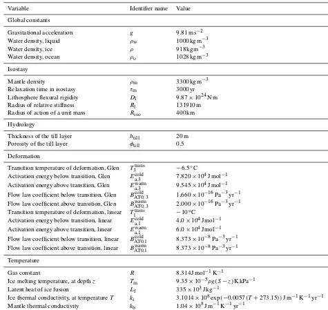
GRISLI constitutive equations were presented in Ritz et al. (2001) and we aim here to give a broad comprehensive de-scription of the current model version, with its latest func-tionalities. Major model parameters are listed in Table 1. 2.1 Ice thermomechanics
2.1.1 Ice deformation and mass conservation
Ice deformation and mass conservation in GRISLI version 2.0 are mostly treated as in Ritz et al. (2001), with the no-table exception of the use of a polynomial flow law with the introduction of a linear, Newtonian viscosity.
GRISLI considers the ice sheet as solely formed of pure ice with a constant and homogeneous density (ρ). In this ap-proximation, the ice being considered as an incompressible fluid, the mass conservation equation can be written as ∇ ·u=∂ux
∂x + ∂uy
∂y + ∂uz
∂z =0, (1)
with ux, uy, uz
Table 1.GRISLI model parameters used in this study.
Variable Identifier name Value
Global constants
Gravitational acceleration g 9.81 m s−2
Water density, liquid ρw 1000 kg m−3
Water density, ice ρ 918 kg m−3
Water density, ocean ρo 1028 kg m−3
Isostasy
Mantle density ρm 3300 kg m−3
Relaxation time in isostasy τm 3000 yr
Lithosphere flexural rigidity Dl 9.87×1024N m
Radius of relative stiffness Rl 131910 m
Radius of action of a unit mass Riso 400 km
Hydrology
Thickness of the till layer htill 20 m
Porosity of the till layer φtill 0.5
Deformation
Transition temperature of deformation, Glen T3trans −6.5◦C
Activation energy below transition, Glen Ea,3cold 7.820×10⁴J mol−1 Activation energy above transition, Glen Ea,3warm 9.545×10⁴J mol−1 Flow law coefficient below transition, Glen BAT0, 3cold 1.660×10⁻¹⁶Pa−3yr−1 Flow law coefficient above transition, Glen BAT0, 3warm 2.000×10⁻¹⁶Pa−3yr−1 Transition temperature of deformation, linear T1trans −10◦C
Activation energy below transition, linear Ea,1cold 4.0×10⁴J mol−1 Activation energy above transition, linear Ea,1warm 6.0×10⁴J mol−1 Flow law coefficient below transition, linear BAT0,1cold 8.373×10⁻⁸Pa−3yr−1 Flow law coefficient above transition, linear BAT0,1warm 8.373×10⁻⁸Pa−3yr−1 Temperature
Gas constant R 8.314 J mol−1K−1
Ice melting temperature, at depthz Tm 9.35×10⁻⁵ρg(S−z)K kPa−1
Latent heat of ice fusion Lf 335×103J kg−1
Ice thermal conductivity, at temperatureT ki 3.1014×10⁸exp(−0.0057(T+273.15))J m−1K−1yr−1 Mantle thermal conductivity kb 1.04×10⁸J m−1K−1yr−1
The vertically integrated expression of the mass conserva-tion equaconserva-tion (Eq. 1) provides the equaconserva-tion for the ice thick-ness,H:
∂H ∂t = −
∂H ux ∂x −
∂H uy
∂y +M−bmelt, (2) withux anduy the vertically integrated velocities inx and y directions,Mthe surface mass balance andbmeltthe basal
melting rate.
The quasi-static approximation is used for the velocity field, in which the inertial terms of the momentum conser-vation equation are ignored. With the gravity force being the sole external force acting on an infinitesimal cube of ice, we
have
∂σx ∂x +
∂τxy ∂y +
∂τxz ∂z =0 ∂τxy
∂x + ∂σy
∂y + ∂τyz
∂z =0 ∂τxz
∂x + ∂τyz
∂y + ∂σz
∂z =ρg
, (3)
where τij=x,y,z are the shearing stress tensor terms and σi=x,y,zthe longitudinal stress tensor terms, defined as (i= x, y, z)
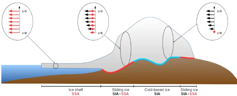
Figure 1.Schematic representation of the different types of flows in GRISLI and their associated velocity profiles. The red arrows stand for the sliding velocity, which is non-zero for temperate-based grounded regions.
The pressure is defined as the first invariant of the stress ten-sor:
−P =σx+σy+σz
3 . (5)
The deviatoric stress tensor is defined as (fori, j=x, y, z)
τij0 =τij+δijP , (6)
withδij being 1 fori=j, and 0 otherwise.
Assuming isotropy, the deviatoric stress and the deforma-tion rateij˙ are related by
τij0 =2ηεij˙, (7)
whereηis the ice viscosity.
Like most ice sheet models, GRISLI considers the ice as a non-Newtonian viscous fluid following a Norton–Hoff con-stitutive law (commonly named Glen flow law):
1
η=BATτ
n−1, (8)
whereBAT is a temperature-dependent coefficient andτ is
the effective shear stress, defined as (fori=x, y, z) τ2=1
2
X
i,j
τij2. (9)
The temperature-dependent coefficientBATis computed
fol-lowing an Arrhenius law: BAT=SfBBAT0exp
E
a
R
1
Tm − 1
T
, (10)
whereSfis a flow enhancement factor,BBAT0is a flow law
coefficient,Eais the activation energy,Ris the gas constant,
Tmis the ice pressure melting temperature, andT is the local
temperature.
To account for the fact that the activation energy increases close to the melting point (Le Gac, 1980), in GRISLI, the pair (Ea,BBAT0) can take two different values for local
tem-peratures higher or lower than a temperature thresholdTtrans (Table 1).
The Glen flow law is an empirical formulation, derived from laboratory experiments. However, laboratory experi-ments cannot cover the full range of deviatoric stress operat-ing in real ice sheets. The timescale over which this stress is applied in real ice sheets is also not reproducible in laborato-ries. Most modelling studies usen=3 for the Glen flow law exponent (Eq. 8). A few studies suggest the possibility for a smaller exponent for small stress regime (Duval and Lli-boutry, 1985; Pimienta, 1987; Pettit and Waddington, 2003). Since the work of Dumas (2002), one specificity of GRISLI is the possibility to simultaneously use a Glen viscosity with n=3 and a linear, Newtonian viscosity withn=1. In this case, the two contributions simply add up:
2ε˙ij=
BAT1+τ2BAT3
τij0, (11)
withBAT1andBAT3computed with Eq. 10, only using
dif-ferent activation energy (Ea,1andEa,3), flow law coefficient
(BBAT0,1 andBBAT3) and temperature threshold (T1trans and
T3trans). The chosen values (Table 1) are based on Lipenkov et al. (1997).
Like other large-scale ice sheet models, GRISLI does not explicitly take into account anisotropy, which tends to facil-itate deformation due to vertical shear, but reduces deforma-tion due to longitudinal stress. The role of the flow enhance-ment factorSfin Eq. (10) is to artificially account for the
ef-fect of anisotropy.Sftakes different values for the two
com-ponents of the velocities computed in GRISLI (due to vertical shearing or longitudinal deformation, presented in the next section). In particular, we use a fixed ratio, typically ranging from 5 : 1 to 10 : 1 (Ma et al., 2010), between the value of the enhancement factorSffor vertical shear and the one for
to 8 : 1 and the enhancement factor Sf for vertical shearing
with a Glen viscosity will be one of the calibrated param-eters. In turn, the flow enhancement factor for the vertical shearing with a linear viscosity is set to 1.
2.1.2 Ice velocity
Differing from Ritz et al. (2001), the velocity in GRISLI is now computed for the entire domain as the superposition of the shallow ice approximation (SIA) and the shallow shelf approximation (SSA) components, without using a sliding law to estimate basal velocities (Fig. 1).
The SIA (Hutter, 1982) assumes that the velocity horizon-tal derivatives are much smaller than its vertical derivatives, which is generally true for the major part of the ice sheet where the gravity-driven flow induces a slow motion of the ice. GRISLI uses a zero-order approximation of the SIA in which the stress tensor components simplify to
τxz=ρg ∂S ∂x(S−z) τyz=ρg∂S
∂y(S−z)
, (12)
withSthe surface elevation. The vertical velocity profile is computed as an integral from the bedrock elevation,B, to a given vertical coordinate,z(fori=x, y):
ui(z)=ui,b+
z
Z
B
2εiz˙ dz, (13)
whereui,bis theicomponent of the basal velocity.
The basal velocity can be computed with a sliding law (e.g. Bindschadler, 1983). However, recent versions of GRISLI use the SSA as a sliding law, as suggested by Bueler and Brown (2009). In this case, similarly to Winkelmann et al. (2011), we simply add up the two contributions of the SIA and SSA for the whole domain which ensure a smooth transi-tion from non-sliding frozen regions to sliding over a thawed bed.
For fast-flowing regions, the vertical stresses are much smaller than the longitudinal shear stresses. In this case, the velocity fields with the SSA (MacAyeal, 1989) reduce to the following elliptic equations:
∂ ∂x
2η H (2 ∂ux ∂x + ∂uy ∂y ) + ∂ ∂y
η H (∂ux ∂y +
∂uy ∂x )
=ρgH ∂S ∂x−τb,x ∂
∂y
2η H (2 ∂uy ∂y + ∂ux ∂x ) + ∂ ∂x
η H (∂uy ∂x +
∂ux ∂y )
=ρgH ∂S ∂y −τb,y
,
(14) whereτbis the basal drag. The velocitiesuxanduyare iden-tical along the veriden-tical dimension.
The condition at the front of the ice shelf is given by the balance between the water pressure and the horizontal longi-tudinal stress (see also Sect. 2.3 on the numerical features).
The code section relative to the elliptic equation is avail-able in the Supplement.
2.1.3 Basal drag
For floating ice shelves, the basal drag,τb, is negligible. For
cold-based grounded ice, we impose a large enough basal drag (typically 105Pa) to ensure virtually no-slip conditions on the bedrock, and the basal velocity is set to zero in this case. For temperate-based grounded ice, a power–law basal friction (Weertman, 1957) is assumed:
τbm,x= −β ub,x τbm,y= −β ub,y
, (15)
where the basal drag coefficientβ is positive. In the experi-ment presented here, we assume the presence of a sediexperi-ment at the base of the ice sheet allowing for a viscous deformation (m=1).
In some recent applications of GRISLI, the basal drag co-efficient has been inferred with an inverse method in order to match present-day ice sheet geometry (Ritz et al., 2015; Le clec’h et al., 2018). This approach has been followed to participate in the first phase of the recent ice sheet model intercomparison project (ISMIP6, Nowicki et al., 2016) for both the Greenland (Goelzer et al., 2017) and Antarctic ice sheets. In this context, GRISLI computes sea level rise pro-jections by the end of the century in line with results from more complex models (Edwards et al., 2014; Goelzer et al., 2017).
Inverse methods are especially suited to produce an ice sheet state (e.g. geometry and/or velocity) close to observa-tions. However, by construction, such methods do not pro-vide information where no ice is present in observations. As such, they are difficult to apply for palaeo reconstructions of the American or Eurasian ice sheets. More generally, inverse methods are no longer appropriate for long-term integrations, either palaeo or future, when ice thickness is very different from its present state and especially if the ice margin mi-grates from its present-day position. This motivates the use of a basal drag coefficient computed from GRISLI internal variables. We generally assume that its value is modulated by the effective water pressure,N, at the base of the ice sheet:
β=CfN, (16)
withCfan internal parameter that needs calibration.
In our approach, any temperate-based grounded point will have a non-zero sliding velocity, depending on theCffactor
sediment thickness exceeds a certain threshold, whilst Qui-quet et al. (2013) restrict this to large-scale valleys. However, these approaches have flaws. For example, the sediment dis-tribution is only poorly known below present-day ice sheets and its past evolution is largely uncertain. Also, the definition of a typical spatial scale for ice streams is somewhat arbi-trary. For these reasons, in the following, we use the simplest approach and compute Eq. (16) for any temperate-based grid point. TheCfparameter will be part of the calibrated
param-eters in our large ensemble. 2.1.4 Flux at the grounding line
In Ritz et al. (2001), the position of the grounding line was computed from a simple floatation criterion with no specific flux computation at the grounding line. Such an approach is in theory only valid for a very high spatial resolution, within tenths of metres, at the vicinity of the grounding line (Durand et al., 2009). Because the model runs typically at a much coarser resolution, in GRISLI version 2.0, we have imple-mented an explicit flux computation at the grounding line based on the analytical formulations from Schoof (2007) and Tsai et al. (2015). The two formulations differ from the as-sumption made on the sediment rheology.
The flux at the grounding line following Schoof (2007) is
qglS = −
A(ρg)n+1(1−ρ/ρw)n
4nβ
m+1m
H
m(n+3)+1 m+1
gl φ
m n m+1
bf , (17)
withnandmbeing the exponents in the Glen flow law (Eq. 8) and in the friction law (Eq. 15) respectively,Athe vertically integrated temperature dependent coefficient in the Glen flow law (BAT, Eq. 8),Hglthe ice thickness at the grounding line,
andφbfa back force coefficient to take into account the
but-tressing role of ice shelves. β is the basal drag coefficient presented in Eq. (15).
Conversely, Tsai et al. (2015) proposed qglT =Q0
8A(ρg)n
4nf (1−ρ/ρw)
n−1Hn+2 gl φ
n−1
bf , (18)
with Q0=0.61. In this case, the basal drag is assumed to
vanish at the grounding and as such the coefficientβ is not used. Instead, Tsai et al. (2015) suggest a constant and ho-mogeneous basal friction coefficientf set to 0.6.
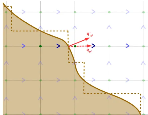
In GRISLI, from the last grounded point in the direction of the flow, we compute the sub-grid position of the grounding line in thexandydirections linearly interpolating the floata-tion criterion (dark green dots in Fig. 2). From this posifloata-tion, the flux at the grounding line is calculated using Eq. (17) or Eq. (18) (red arrows in Fig. 2). Because the flux at the sub-grid position is perpendicular to the local grounding line, ideally we should project this flux onto the x and y axes. However, in the model, we assume that the grounding line is always perpendicular to either thexoryaxis (dashed brown line in Fig. 2). As in Fürst (2013), the value of the fluxqglis
Figure 2.Horizontal staggered grids used in the model. The blue arrows stand for the staggered velocity grid, while the green circles represent the standard centred grid (for, e.g. ice thickness, temper-ature, effective pressure). The plain brown line is an illustration of the grounding line position with an example of the flux (qgl0 ) at one location where the grounding line crosses thexaxis in the centred grid. In the model, the norm of the flux at this location is reported on theuvelocity only (qgl), i.e. assuming a grounding line perpendic-ular to thexaxis (dashed brown line). The dark blue arrows are the velocity nodes on whichqglis interpolated, using the velocity val-ues of the two bounding light blue arrows. The dark green dots are used to infer the sub-grid position of the grounding, interpolating the floatation criterion (ρH+ρw(B−sealevel)).
linearly interpolated to the two closest downstream and up-stream velocity grid points (dark blue arrows in Fig. 2) using the two bounding velocity points (light blue arrows in Fig. 2). To evaluate the back force coefficientφbf, we solve the
ve-locity equation twice. The first iteration is computed on the simulated geometry with no specific flux adjustment at the grounding line (i.e. not using Eq. 17 or 18). The second iter-ation is computed the same way, except for the fact that the ice shelves are assigned to a very low viscosity so that they cannot exert any back force. The buttressing ratio (φbf) is
then computed as the velocity ratio between these two com-puted velocities. Onceφbfis estimated, we solve the velocity
equation again, this time imposing the grounding line flux computation using Eq. (17) or (18), in order to estimate the velocity used in the mass conservation for this time step. We acknowledge the fact that this approach is computationally expensive but it allows for more accurate estimation of the buttressing role of ice shelves in the model.
The code for the implementation of the flux at the ground-ing line in GRISLI is available in the Supplement.
2.1.5 Calving
sim-ple scheme can prevent ice shelf extension, we also maintain downstream ice shelf grid points neighbouring the last grid points meeting the criterion. The cut-off threshold may vary in space (e.g. oceanic depth dependency) and time. In the following, we use a constant and homogeneous thickness cri-terion (set to 250 m, roughly corresponding to the observed present-day Antarctic ice shelves’ front).
2.1.6 Ice temperature calculation
The ice temperature calculation has remained identical to Ritz et al. (2001). As in most large-scale ice sheet models (e.g. Winkelmann et al., 2011; Pollard and DeConto, 2012; Pattyn, 2017), the temperature in GRISLI is computed by solving the general advection–diffusion equation of temper-ature: ∂T ∂t = 1 ρc ∂ ∂x ki ∂T ∂x + 1 ρc ∂ ∂y ki ∂T ∂y
| {z }
horizontal diffusion (19) + 1 ρc ∂ ∂z ki ∂T ∂z
| {z }
vertical diffusion
−ux∂T ∂x −uy
∂T ∂y
| {z }
horizontal advection
− uz∂T
∂z
| {z } vertical advection + Q ρc |{z} heat production ,
withkithe thermal conductivity of the ice,cthe heat capacity
anduzthe vertical velocity, computed as in Ritz et al. (1997) (wtin Eq. 14 of the original paper).
Horizontal diffusion is assumed to be negligible relative to the vertical diffusion.
The heat production is given by Hutter (1983) (fori, j= x, y, z):
Q=X i,j
˙
εijτij. (20)
At the ice sheet surface, due to the absence of an explicit snowpack model, ice temperature is assumed to be equal to the near-surface annual air temperature (but not greater than the melting point). Depending on the surface mass balance parameterisation, the latent heat release due to refreezing is transferred to the first ice layer.
A geothermal heat fluxφ0is applied at the base of a 3 km
thick bedrock layer with a Neumann boundary condition: φ0= −kb
∂T ∂z bedrock , (21)
withkbthe bedrock thermal conductivity.
The heat equation is solved in the bedrock similarly to Eq. (19) but with no advection nor heat production. From the temperature gradient in the bedrock (computed on four
vertical levels), we compute a heat fluxφ00at the ice–bedrock interface. When ice dragging occurs over the bedrock, an ad-ditional term due to friction,φf, is added toφ00:
φf= |ubτb|. (22)
The ice–bedrock interface heat flux is used differently for cold- and temperate-based points:
– For cold-based points, the heat at the ice–bedrock inter-face is transferred to the ice via a Neumann boundary condition: ki ∂T ∂z ice
= −φ00−φf, (23)
with the ice thermal conductivitykicomputed as
ki=3.1014×10⁸ exp(−0.0057(T+273.15)). (24)
– For temperate points, a Dirichlet boundary condition is applied as the temperature is kept at the pressure melt-ing point. The excess heat in this case is used to compute basal melting:
bmelt=
−φ00−φf−ki∂T∂z ice
Lfρ
, (25)
withLfis the latent heat of fusion.
Basal melting for oceanic points is usually imposed. For specific applications, we have different values for deep-ocean and continental shelves, or a geographical distri-bution depending on the oceanic basin.
The viscosity for the velocity grid points is the horizontal av-erage of the viscosity on the centred grid and not the viscos-ity computed from the horizontal average of the temperature. This is preferable for regions with mixed frozen and temper-ate basal conditions.
2.2 Additional features 2.2.1 Basal hydrology
Peyaud (2006) added a simple diffusive basal hydrology scheme in GRISLI. In the following, we provide a com-plete description of the hydrology model because it has only been described in a French PhD dissertation (Peyaud, 2006) but currently lacks a description in an international scientific journal.
Using a Darcy law, the water produced by melting at the base of the ice sheet is routed outside glaciated areas follow-ing the highest gradient in the total water potential.
wherehwis the hydraulic head,Bis the bedrock height, and
H is the ice thickness.
In GRISLI, we assume that the basal water flows within a sub-glacial till following a Darcy-type flow law:
Qw= −KD ρwg
∇8, (27)
whereQw is the water flux vector inx andy directions,K is the hydraulic conductivity of the till, and Dis the water thickness within the till.
The till is assumed to be present everywhere below the ice sheet with a constant and homogeneous thickness (htill=
20 m) and porosity (φtill=0.5). The water thickness in the
till,D, is equivalent to the hydraulic head,hw, only for
thick-nesses lower than the effective thickness:
D=min(hw, φtillhtill). (28)
The hydraulic conductivity of the till,K, is modulated by the effective pressure to take into account sediment dilatation:
K=
K0 ifN > N0
K0N0/N ifN≤N0
, (29)
withK0the reference conductivity,N the effective pressure
andN0 a constant (108Pa). The conductivityK0 is poorly
constrained and strongly depends on the material.
In GRISLI, we assume that the flow of water within the till can be described with a diffusivity equation for the hydraulic head:
∂hw
∂t + ∇ ·Qw=bmelt−Igr, (30)
withIgr being the infiltration rate in the bedrock (kept
con-stant at 1 mm yr−1).
Using Eqs. (26) and (27), this diffusivity equation can be written as
∂hw
∂t =bmelt−Igr+ ∇ ·
KD∇
B+ ρ ρw
H
(31) + ∇ ·(KD∇hw) .
Equation (31) can be solved using a semi-implicit relaxation method as used for the mass conservation equation.
From the hydraulic head, hw, we can compute the
wa-ter pressure,pw=ρwg hw, and the effective pressure,N=
ρg H−pw.
Fortran modules for the basal hydrology are available in the Supplement.
2.2.2 Isostasy
As in Ritz et al. (2001), GRISLI computes the bedrock response to ice load with an elastic lithosphere – relaxed asthenosphere (ELRA) model (Le Meur and Huybrechts,
1996). This simple model evaluates the bedrock deforma-tion to a local unit mass, scaled to the whole ice sheet. The relaxation time of the asthenosphere is usually set to 3000 years and the deflection of the lithosphere is assumed to fol-low a zero-order Kelvin function. Such a simple model has been shown to perform well compared to more sophisticated glacio-isostatic models (Le Meur and Huybrechts, 1996). 2.2.3 Passive tracer
GRISLI includes a passive tracer model that allows for the computation of vertical ice stratigraphy, i.e. time and loca-tion of ice deposiloca-tion for the vertical model grid points. The model is the one of Lhomme et al. (2005), re-implemented in GRISLI by Quiquet et al. (2013). We use a semi-Lagrangian scheme following Clark and Mix (2002) in order to avoid the numerical instabilities of Eulerian schemes and infor-mation dispersion of Lagrangian schemes (Rybak and Huy-brechts, 2003). For each time step, the back trajectories of each grid points are computed and trilinearly interpolated onto the model grid. This allows for continuous information within the ice sheet at a low computational cost. Time and lo-cation of ice deposition can be convoluted, for example, with isotopic composition of precipitation (e.g.δ18O) in order to construct synthetic ice cores comparable to actual ice cores (Lhomme et al., 2005).
The GRISLI code section related to the passive tracers is available in the Supplement.
2.3 Numerical features
The model uses finite differences computed on a staggered Arakawa C grid in the horizontal plane (Fig. 2). In the verti-cal, the model definesσ-reduced coordinates,ζ =(S−z)/H, for 21 evenly spaced vertical layers, with thezvertical axis pointing upward andζ pointing downward (0 at the surface and 1 at the bottom). The coordinate triplet(i, j, k)(inx,y andζ directions) is representative of the centre of the grid cell. The horizontal resolution depends on the application, i.e. the extension of the geographical domain and the dura-tion of the simulated period. For century-scale applicadura-tions, the resolution varies from 5 km for Greenland to 15 km for Antarctica (Peano et al., 2017; Ritz et al., 2015). For multi-millennial applications, the resolution is reduced to 15 km for Greenland and 40 km for the whole Northern Hemisphere and Antarctica.
grid. Note that this smaller time step is solely used for the mass conservation equation (Eq. 2) and subsequent variables (e.g. surface slopes, SIA velocity), while the rest of the model uses a main time step, typically ranging from 0.5 to 5 years depending on the horizontal resolution.
To solve the ice shelf/ice stream equation, Eq. (14) needs to be linearised. The viscosity is computed using an itera-tive method starting from the viscosity calculated from strain rates from the previous time step. As this equation is the most expensive part of the model, the iteration mode is not always used depending on the type of experiment (for in-stance, not crucial when the objective is to reach a steady state). In this case, the viscosity of the previous time step is used. The linear system is solved with a direct method (Gaussian elimination, sgbsv in the Lapack library; http: //www.netlib.org/lapack/, last access: 3 December 2018).
The resolution of the elliptic system (Eq. 14) is the most expensive part of the model. This is further amplified by the way we prescribe boundary conditions. As in Ritz et al. (2001), the ice shelf region is artificially extended towards the edges of the geographical domain. This artificial exten-sion does not have any consequence on ice shelf velocity since added grid points (that we call “ghost” nodes) are pre-scribed with a negligible ice viscosity (1500 Pa s). The front is then parallel to either x ory (Ritz et al., 2001), and thus the boundary condition there is easy to implement (see also Fig. S1 in the Supplement). The boundary condition at the real ice shelf front is solved implicitly with Eq. (14). How-ever, this method substantially increases the size of the linear system solved in Eq. (14). To circumvent this issue, a sim-ple reduction method is imsim-plemented. Equation (14) can be written aseAeu=eB, whereeuis a vector alternatingux and
uy components for all the velocity grid points,eAis a band
matrix (very sparse), andBeis a vector corresponding to the
right-hand terms in Eq. (14). Every line ofeAandBeis scaled
so that the diagonal terms ofeAare equal to 1. If, for a given
velocity node, all the non-diagonal terms of the column are very small compared to 1, this means that this node is in prac-tice not used by any other velocity node and this line of the matrix can be removed. The threshold to neglect nodes is re-lated to the value of the integrated viscosity of ghost nodes. In practice, given its size, the matrixeAis not fully populated,
being a band matrix with a bandwidth of 1. An illustration of the matrix is shown in Fig. S2 in the Supplement, while the Fortran files are available (“New-remplimat” directory).
For the temperature equation (Eq. 19), we solved a 1-D advection–diffusion equation for each model grid point. The resolution is performed with an upwind semi-implicit scheme (vertical velocity and heat production at the previous time step is used). The ice thermal conductivity is computed as the geometric mean of the two neighbouring conductivi-ties (Patankar, 1980). Because the horizontal diffusion is ne-glected, the only horizontal terms concern horizontal advec-tion and are computed with an upwind explicit scheme. The heat production is computed at the velocity (staggered) grid
points and is then summed up to the temperature (centred) grid points.
The model has been recently partially parallelised with OpenMP (https://www.openmp.org/, last access: 3 December 2018), which considerably shortens the length of the simula-tions (gain of 40 % for the Antarctic at 40 km on four threads of an Intel®Xeon®CPU at 3.47 GHz).
3 Calibration for the Antarctic ice sheet
Over the years, several GRISLI internal parameters have been shown to be of importance to appropriately simulate the flow and mass balance of the Antarctic ice sheet. Val-ues for these parameters have been so far derived from non-systematic tests and expert knowledge. To non-systematically in-vestigate the role of those parameters and find the best fit-ting set for the simulated Antarctic ice sheet with respect to the observed one, a calibration methodology with system-atic exploration of the different values is performed in the following. The best fitting set will be considered as plau-sible models within the chosen parameter space. Given its degree of complexity, GRISLI is mostly designed for multi-millennial integrations. Due to long-term diffusive response to SMB and temperature changes, an accurate methodology to select unknown parameters of the model would be to run long transient simulations with a climate forcing as close as possible to past climate states, ideally with a synchronous coupling between the ice sheet and the atmosphere. How-ever, climate models generally fail at reproducing the re-gional climate changes during the last glacial–interglacial cycle as recorded by proxy data (Braconnot et al., 2012). Furthermore, the phase III of the Paleoclimate Modelling Intercomparison Project (PMIP3) has highlighted the large disagreement between participating climate models in sim-ulating the Last Glacial Maximum (LGM) in the vicinity of Northern Hemisphere ice sheets (e.g. Harrison et al., 2014). Given these uncertainties amongst climate models and the large sensitivity of the ice sheet model to climate forcing fields (e.g. Charbit et al., 2007; Quiquet et al., 2012; Yan et al., 2013), it is difficult to calibrate the mechanical param-eters independently from those of the SMB, in particular for Northern Hemisphere ice sheets. For these reasons, here we suggest a simple calibration methodology for the Antarctic ice sheet in which the model is run for 100 kyr under a per-petual modern climate forcing until equilibrium.
3.1 Methods
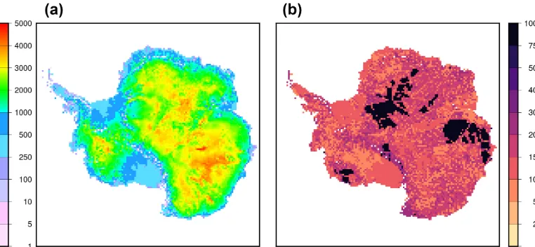
Figure 3.Antarctic ice shelf sectors(a)and associated prescribed present-day sub-shelf basal melting rates in m yr−1(b). The melting rates are different for the shelf and the associated grounding line to mimic the higher values observed close to the grounding line (Rignot et al., 2013). Sub-shelf melting rates for the deep ocean (depth greater than 2500 m) are assigned a value of 5 m yr−1.
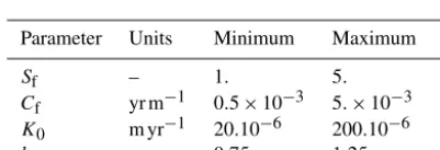
Table 2.Selected parameters included in the Latin hypercube sam-pling (LHS) ensemble with their associated ranges.
Parameter Units Minimum Maximum
Sf – 1. 5.
Cf yr m−1 0.5×10⁻³ 5.×10−3
K0 m yr−1 20.10−6 200.10−6
bmelt – 0.75 1.25
project (Nowicki et al., 2016) and are shown in Fig. 3. Their values are based on the sectoral average of sub-shelf melt rates that ensured stable ice shelves (minimal Eulerian ice thickness derivative) in the recent intercomparison exercise InitMIP-Antarctica (Nowicki et al., 2016), with slight mod-ifications due to change in resolution. They are in line with observation-based estimates (Rignot et al., 2013). We do not apply any correction related to geometry changes to the cli-matic forcings during the calibration.
We choose to restrict this study to a coarse horizontal res-olution, namely 40 km, as it allows for large ensembles of multi-millennial simulations. Whilst 6.7 h on one thread of an Intel®Xeon®CPU at 3.47 GHz (4 h on four threads) are needed to perform 100 000 years of simulation over Antarc-tica on a 40 km grid (19 881 horizontal grid points), this time goes up significantly on a 16 km grid (145 161 points) for which we need 25 h to perform 2000 years (17 h on four threads). In addition, the 40 km resolution corresponds to the one used in the coupled version within theiLOVECLIM Earth system model of intermediate complexity (Roche et al., 2014). Whilst with such a resolution we do not expect to have an accurate representation of the ice sheet fine-scale struc-tures such as ice streams, we expect to reproduce the large-scale behaviour of ice flow.
From our experience with GRISLI, we identified four un-known independent parameters that have a crucial role for ice dynamics:
– The SIA flow enhancement factorSf of the Glen flow
law (Eq. 10) is expected to have a large influence on shear-stress-driven velocities.
– The basal drag coefficientCfin Eq. (16) is used to
mod-ulate the basal drag coefficient for temperate-based grid points where sliding occurs.
– The till conductivityK0changes the efficiency of basal
water routing (Eqs. 29 and 31) and thus basal effec-tive pressureN. As such, this parameter also influences the basal drag coefficientβfor temperate-based regions (Eq. 16).
– An ice shelf basal melting rate coefficient φshelf
indi-cates, for a specific Antarctic ice shelf sectori,
BMBi=φshelfBMBi0, (32)
with BMBi0 the sub-shelf basal melting rate reference values shown in Fig. 3.
Figure 4.Bedmap2 ice thickness(a)and associated uncertainty(b)in metres (Fretwell et al., 2013), interpolated on the GRISLI grid of Antarctica at 40 km resolution. Despite considerable improvements from Bedmap1, large areas present an important uncertainty (±1000 m) due essentially to poor in situ data coverage.
Figure 5.Simulated total ice volume for each ensemble members as a function of parameter values when using the Schoof (2007) formu-lation of the flux at the grounding line (AN40S). The thick horizon-tal line shows the observations (Fretwell et al., 2013). The colour shading corresponds to the root mean square error in ice thickness relative to observations. The stars outlined in red are the 12 ensem-ble members having the lowest RMSE.
The initial ice sheet geometry, bedrock and ice thickness, is taken from the Bedmap2 dataset (Fretwell et al., 2013, Fig. 4) using a spatial bilinear interpolation to generate these data on the 40 km grid. The geothermal heat flux is from Shapiro and Ritzwoller (2004). Sensitivity to uncertainties in the forcing data is not explored in the ensemble as we aim at quantifying the model sensitivity to parameter choice even though we acknowledge the fact that these could be the source of important model error (e.g. Stone et al., 2010; Pol-lard and DeConto, 2012).
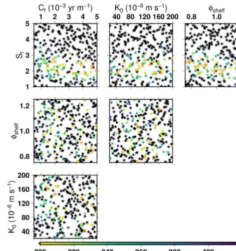
Figure 6.Same as Fig. 5 but with the Tsai et al. (2015) formulation of the flux at the grounding line (AN40T).
Figure 7.Ice thickness difference with the observations in metres (simulated minus observed) from the 12 ensemble members showing the lowest RMSE when using the Schoof (2007) formulation of the flux at the grounding line (AN40S).
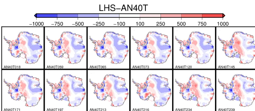
Figure 8.Same as Fig. 7 but with the Tsai et al. (2015) formulation of the flux at the grounding line (AN40T).
also reduce the error in velocities with respect to observations at the global scale.
3.2 Calibration results
Figure 5 presents the Antarctic ice sheet volumes at the end of the 100 kyr simulations for each ensemble member as a function of parameter values using the flux at the grounding line computed from Schoof (2007) (AN40S). We can see that there is a strong positive (respectively, negative) correlation of ice volume with the basal drag coefficient (respectively, enhancement factor). There is also a weak negative correla-tion for the sub-shelf basal melt coefficient and a weak pos-itive correlation with the till conductivity. Since the global volume is an integrated metric that does not account for po-tential systematic compensation, in Fig. 5 we also show the RMSE in ice thickness for each ensemble member with re-spect to observations (Fretwell et al., 2013). Amongst the
300 model realisations, 120 members have a RMSE lower than 350 m. These members are widely distributed within the member spectrum. The lowest RMSE is 294 m. The 12 best ensemble members are outlined in red in Fig. 5 and have a RMSE not higher than 304.
Figure 9. Ice thickness root mean square error respective to ob-servations in the parameter space for the 300 model members us-ing the Schoof (2007) formulation of the flux at the groundus-ing line (AN40S). The 12 experiments showing the lowest error are outlined in red.
amplifying the role of the ice flow enhancement factor. As a consequence, for the AN40T ensemble, the enhancement factor requires values between 1.5 and 3 in order to reach good agreement with observed ice thickness, whilst values within 1.5 to 4 are acceptable for AN40S.
In Fig. 7 (respectively, Fig. 8), we show the ice thickness difference from the observations for the 12 ensemble mem-bers showing the lowest RMSE within the AN40S (respec-tively, AN40T) model realisations. The differences are gener-ally below 500 m even if persisting model biases are present across the ensemble members and model formulations. On the one hand, ice thickness in large parts of the East Antarc-tic ice sheet is systemaAntarc-tically underestimated. On the other hand, the West Antarctic ice sheet shows more contrasted responses. Whilst for some ensemble members, the Ross embayment upstream region can be well represented (e.g. AN40S004 or AN40T065), the region feeding the Filchner– Ronne ice shelf shows a quasi-systematic ice thickness un-derestimation. These model deficiencies can be attributed to our coarse model resolution, providing a poor represen-tation of the complex bedrock structure in the Filchner– Ronne area. The model differences from the observations are very similar to results from the Potsdam Parallel Ice Sheet Model (PISM-PIK) shown in Martin et al. (2011) in terms of amplitude but also in terms of structure. They are also generally similar to Pollard and DeConto (2009). Consistent model biases amongst these models, which use different
in-Figure 10.Same as Fig. 9 but with the Tsai et al. (2015) formulation of the flux at the grounding line (AN40T).
put data, suggest a common source of error related to the coarse model resolution (20 to 40 km) or uncertainties in the bedrock dataset, particularly large in East Antarctica (Fig. 4). Figure 9 (respectively, Fig. 10) presents the root mean square error with respect to observations of the ensemble members in the two-dimensional parametric space within AN40S (respectively, AN40T). The 12 best ensemble mem-bers are outlined in red. In most cases, there is no clear re-lationship. However, there is a relationship emerging with a large basal drag coefficient being compensated by a large enhancement factor when using the Schoof (2007) formula-tion (Fig. 9). When using the Tsai et al. (2015) formulaformula-tion (Fig. 10), this relationship disappears, as the enhancement factor is mostly driving the model response. A few model parameter combinations (30 out of 300) are able to provide a good representation of the present-day Antarctic ice sheet, i.e. RMSE lower than 350 m, independently from the ground-ing flux computation used (not shown).
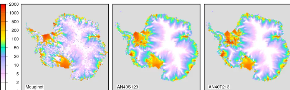
Figure 11.Observed velocity (Mouginot et al., 2017) against modelled velocity on the 40 km grid. Only the best ensemble members with the lowest RMSE are shown here for Schoof (2007) (AN40S123,a) and Tsai et al. (2015) (AN40T213,b). The parameter values for these experiments are shown in Table 3.
Figure 12.Map of observed (Mouginot et al., 2017) and simulated velocities in m yr−1for the ensemble members with the lowest RMSE using Schoof (2007) (AN40S123) and Tsai et al. (2015) (AN40T213).
to the coarse resolution used but also to the simple scheme used to estimate basal drag.
From each of the two ensembles (AN40S and AN40T), we keep the 12 ensemble members out of 300 that have the lowest RMSE and use them in the next section for transient simulations covering the last 400 kyr. Using these 24 plau-sible models on long-term transient integration provides in-sight on the GRISLI result spread for models yielding a sim-ilar present-day ice sheet. Indeed, while they have a simsim-ilar RMSE, they have distinct parameter values (Figs. 5 and 6) and as such they provide insight on the uncertainties in ice sheet evolution relative to parameter choice. We acknowl-edge that the choice of 12×2 ensemble members is arbitrary and this number is too low to infer statistically meaningful results in terms of model uncertainty. Still, even with our relatively coarse resolution, 400 kyr simulations represent a non-negligible computing time that has to be added to the 600 ensemble members of Sect. 3.
4 Antarctic ice sheet changes for the last 400 kyr 4.1 Methods
Table 3.Parameter values for the ensemble members that yield the lowest RMSE with respect to observations at the end of the 100 kyr simulation under perpetual present-day climate forcing.
Ensemble member Sf Cf(yr m−1) K0(m yr−1) φshelf Using Schoof (2007) 123 3.19 2.4×10⁻³ 188×10−6 1.05 Using Tsai et al. (2015) 213 2.33 4.6×10⁻³ 114×10−6 0.86
The near-surface air temperature, used in the model as a surface boundary condition for the advection–diffusion tem-perature equation, is assumed to follow the European Project for Ice Coring in Antarctica (EPICA) Dome C deuterium record (δD):
Tpalaeo=T0+
1/αiδD, (33)
withT0 the annual mean near-surface air temperature from
RACMO2.3 used for the present-day calibration. The iso-topic slope for temperature, αi, is set to 0.18 ‰◦C−1 as in Jouzel et al. (2007).
We also account for the additional temperature perturba-tion due to topography changes using a fixed and homoge-neous lapse rate (λ):
Tpalaeo∗ =Tpalaeo+λ (S−S0) , (34)
withS−S0the local topography change from Bedmap2. In
the following,λis set to−8◦C km−1.
For a given near-surface air temperature change Tpalaeo∗ relative to present-dayT0, we modify the present-day SMB
field, SMB0:
SMB=SMB0exp
−γT0−Tpalaeo∗
, (35)
with the precipitation ratio to temperature change γ set to 0.07◦C−1. The use of an exponential form in Eq. (35) is mo-tivated by the Clausius–Clapeyron saturation vapour pressure for an ideal gas. Such a simple expression implies that SMB is driven only by accumulation, an assumption justified by the very little surface ablation experienced by the Antarc-tic ice sheet under present-day climaAntarc-tic conditions. However, we may underestimate the surface melt for warmer past in-terglacial periods.
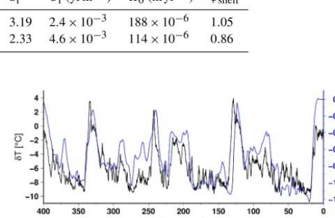
In order to account for changes in basal melting rates be-low ice shelves, there is the need to define a continuous proxy covering several glacial–interglacial cycles for past sub-surface oceanic conditions around Antarctica. To this end, and due to the lack of such a record in the South-ern Ocean, we used the temperature derived from a ben-thic foraminifer δ18O record from the North Atlantic. This temperature signal is considered to depict the North Atlantic Deep Water (NADW) temperature (Waelbroeck et al., 2002). Here, we assume that changes in NADW temperature drive changes in the temperature of waters upwelled in the South-ern Ocean. This upward flow separates into surface equator-ward and poleequator-ward flows, and thus influences surface and
Figure 13. Climatic perturbation used in the 400 kyr glacial– interglacial simulations for the near-surface air temperature,δT =
1/αi
δD, and for the sub-shelf basal melting rate modifier,δoc= αoc1TNA/TNA0.
sub-surface temperature around coastal Antarctica (e.g. Fer-rari et al., 2014). The basal melting rate below a specific ice shelf sectori, BMBipalaeofor past periods is computed from its present-day value, BMBi0, corrected to account for past oceanic conditions:
BMBipalaeo=maxBMBi0 1+δoc
,0.01 m yr−1, (36) using the palaeo-oceanic indexδocdefined as
δoc=αoc1TNA/TNA0, (37)
withTNA0the pre-industrial temperature deduced from North
Atlantic benthic foraminifera (Waelbroeck et al., 2002) and 1TNAthe deviation from this temperature in the past.αocis
a conversion coefficient, set to 1 in the following.
The atmospheric and oceanic indexes, Tpalaeo−T0 and
δoc, used to drive the model for the last 400 kyr are pre-sented in Fig. 13. In addition to these climatic perturba-tions, we also use the eustatic sea level reconstruction of Waelbroeck et al. (2002) to account for sea level variations over glacial–interglacial cycles.
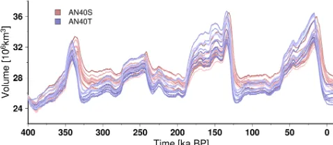
Figure 14.Simulated total ice sheet volume evolution over the last 400 kyr for the 12 ensemble members showing the lowest RMSE in Sect. 3 when using the flux at the grounding line computed from Schoof (2007) (AN40S, shades of red) and Tsai et al. (2015) (AN40T, shades of blue). The glacial–interglacial difference in ice volume for the last termination corresponds to about−10 to−20 m of global sea level rise equivalent depending on the simulations.
4.2 Transient simulation results
In Fig. 14, the simulated ice sheet volume is shown over the last 400 kyr. Across this timescale, a large glacial– interglacial volume variation is observed, in particular for the last two cycles, where it reaches up to about 10 million km3. In our simulations, the Antarctic ice sheet volume increase at the LGM (21 ka BP) relative to pre-industrial corresponds to about−10 to−20 m of global eustatic sea level drop de-pending on the simulations. These numbers mostly fall in the range of previous ice sheet model reconstructions (e.g. Huybrechts, 2002; Philippon et al., 2006; Pollard and De-Conto, 2009), Antarctic contributions inferred as the dif-ference from far-field and Northern Hemisphere near-field estimates (Peltier, 2004) or near-field estimates (Ivins and James, 2005; Argus et al., 2014; Whitehouse et al., 2012; Briggs et al., 2014). Our reconstructions are nonetheless at the higher end of recent studies. This could be related to the fact that we do not account for different geologic bed types today between ice-free (with extensive amount of deformable till) and glaciated (mostly hard bed) continental shelf. To ac-count for this, some authors have chosen a two-value basal drag for these different regions (e.g. Pollard and DeConto, 2012). Because of the large uncertainties related to the bed properties, we have decided to ignore these differences, keep-ing in mind that this can bias our results towards thicker ice sheet when the ice expands over the continental shelf. In our simulations, the last interglacial (120 ka BP) ice volume has no substantial changes relative to the present-day ice volume, with the Antarctic ice sheet contributing less than 6 cm to the global eustatic sea level rise in the simulations with the lowest RMSE at 0 ka. This is well below recent estimates, ranging from 3 to 7 m, inferred from the limited contribution of Greenland to the last interglacial highstand (Dutton et al., 2015). Our crude representation of the last interglacial cli-mate in which no surface melt is possible may be the cause
for such a discrepancy. In addition, our proxy-based basal melting rate does not allow for higher-than-present basal melting rates during the last interglacial.
The uncertainty related to the choice of the internal param-eters within our subset leads generally to up to 3×10⁶km3 differences in our framework but does not change the model response to the forcings. In turn, the choice of either Schoof (2007) (AN40S) or Tsai et al. (2015) (AN40T) to compute the flux at the grounding line leads to important differences amongst temporal model responses. AN40T systematically start to retreat before AN40S. It also produces a larger glacial to interglacial volume change. This confirms the fact that the Tsai et al. (2015) formulation leads to higher grounding line migration variability as already highlighted in Sect. 3 and by other authors (Pattyn, 2017). The additional 10 kyr into the future with no climatic perturbation shows that the AN40S ensemble members do not produce an ice sheet at equilibrium at 0 ka BP. This means that, in our model, the Schoof (2007) formulation produces unrealistically too-slow post-LGM retreat, which induces a model drift persisting till 10 kyr in the future. Conversely, the Tsai et al. (2015) for-mulation leads to more rapid retreat rates, which provides a stabilisation of the ice sheet during the Holocene.
Simulated ice sheet surface elevations at selected snap-shots for the two ensemble members with the lowest RMSE at 0 ka BP after the transient simulations are presented in Fig. 15. Ice sheet geometry during the last interglacial re-sembles the present-day one. This is particularly true for the eastern part, whilst the West Antarctic ice sheet is only slightly thinner. At the Last Glacial Maximum, the ground-ing line advances towards the edge of the continental shelf, in agreement with geological reconstructions (Bentley et al., 2014). The choice of the flux at the grounding line formu-lation has an impact on the maximum ice sheet extent, with a less extended ice sheet using the Schoof (2007) formula-tion. As for the last interglacial, the eastern part of the ice sheet presents only small variations in surface elevation com-pared to the present-day geometry. There is no decrease in surface elevation at the Last Glacial Maximum due to reduc-tion in precipitareduc-tion at this time since the larger extent and the colder climate tend to reduce the ice flow. The largest to-pography changes occur in the Weddell and Ross seas. The West Antarctic ice sheet is thus particularly dynamic during glacial–interglacial cycles.
Figure 15.Simulated surface elevation at selected snapshots for the two ensemble members that produce the minimal RMSE at 0 ka BP in the transient simulations: AN40S252(a)and AN40T213(b). The ice volume contributing to sea level change from the present is−9.3 m (respectively, −15.1 m) at 21 ka BP for AN40S252 (respectively, AN40T213), whilst it is limited at 120 ka BP (−0.3 and+0.6 m). The grounding line is indicated by the thick red line.
Figure 16.Ice thickness difference with the observations (simulated minus observed) at 0 ka BP for the two ensemble members that produce the minimal RMSE at 0 ka BP in the transient simulations: AN40S252(a)and AN40T213(b). The RMSE is 350 m (respectively, 313 m) for AN40S252 (respectively, AN40T213).
corrected when performing a transient simulation. This could be the result of a better representation of the temperature ver-tical profile in this case. On the other hand, whilst in other regions the model biases remain generally the same between an equilibrium and a transient simulation, important model biases appear at the margins of the ice sheet when using
5 Discussion and outlook
We have presented results from the updated version of the GRISLI model. Whilst the model is able to reproduce present-day Greenland (Le clec’h et al., 2017) and Antarctic (Ritz et al., 2015) ice sheets when using an inverse method to estimate the basal drag, our simulations with interactive basal drag coefficients computed from the effective pressure show some important disagreement relative to observations. In particular, there are some persisting model biases in ice thickness. In East Antarctica, the ice thickness is underes-timated towards the pole and the Transantarctic Mountains while it is overestimated towards the margins, from Queen Maud Land to Wilkes Land. In West Antarctica, there is an underestimation of ice thickness in the Filchner–Ronne basin and an overestimation in the Ross basin. These model bi-ases are also present in models of similar complexity when using an interactive basal drag computation (Pollard and De-Conto, 2009; Martin et al., 2011). This data–model mismatch is mostly due to a poor representation of the ice–bedrock in-terface. In particular, the coarse resolution does not allow for the consideration of fine-scale troughs and pinning points. The persisting model biases can also be the consequence of our simplified basal drag computation that does not take into account bedrock physical properties (e.g. sediments).
We used a basal drag coefficient computed from an in-ternal model parameter, namely the basal effective pressure. For long-term multi-millennial integrations, this is preferred to deducing the basal drag coefficient from inversion using present-day geometry since it is fully consistent with the model physics and, in principle, remains valid for large ice sheet geometry change. However, by design, the fit with ob-servations is systematically poorer compared to model re-sults that make use of an inverse basal drag coefficient. A step forward would be to use the basal drag computed from inversion in order to deduce a formulation based solely on internal parameters. Amongst these parameters, along with the basal effective pressure, the large-scale bedrock curva-ture and/or sub-grid roughness could be used, as in Briggs et al. (2013). However, some key basal features, such as the geologic bed type and the deformable till distribution, remain largely unknown today below present-day ice sheets and will contribute to large uncertainties in the basal drag formula-tion.
Although widely used for ice sheet model spin-up or calibration, long-term integrations under present-day forc-ing induce a warm bias in the vertical temperature pro-file because they discard the diffusion of glacial–interglacial changes in surface temperature. Calibrated parameters ob-tained with such a methodology tend to compensate for the underestimated viscosity and are in theory not suitable for palaeo-reconstructions. Whilst a parameter calibration based on glacial–interglacial simulations is ideally preferred, the determination of a realistic climate forcing is a considerable challenge given the many degrees of freedom. Here, we
pre-sented a very simplified climate reconstructions for the last 400 kyr based on a minimal parameter set (proxy for atmo-spheric temperatures and oceanic conditions) in order to il-lustrate the possible model behaviour for long-term integra-tions. Using the parameters calibrated under perpetual mod-ern climate, the model is nonetheless able to reproduce ice geometry changes compatible with palaeo-constraints. Fur-ther work will consist in the determination of more realistic climate reconstruction using general circulation model snap-shots. We also aim to expand the work of Roche et al. (2014) and couple the Antarctic geometry of GRISLI version 2.0 with theiLOVECLIM model.
The implementation of an explicit flux computation at the grounding line following Schoof (2007) and Tsai et al. (2015) led to a more dynamic grounding line position com-pared to previous version of the model. As such, GRISLI version 2.0 is now more sensitive to both sub-shelf melt rate changes and also sea level variations. However, the current version of the model only considers a eustatic sea level per-turbation with a regional bedrock adjustment. The explicit computation of local relative sea level could potentially have an important impact on grounding line migration for glacial– interglacial cycles (e.g. Gomez et al., 2013).
In the current version of the model, some important pro-cesses are still largely simplified. In particular, further devel-opments will consist in the implementation of a new basal hydrology model relying on an explicit routing scheme (e.g. Kavanagh and Tarasov, 2017) avoiding relaxed numerical solutions based on effective pressure. This could introduce fast basal water changes that are currently ignored and, ulti-mately, yield the abrupt speeding up or slowing down of ice streams. Also, calving processes are suspected to be a major driver for ice sheet evolution due to the importance of but-tressing on inland ice dynamics (e.g. Pollard et al., 2015). GRISLI version 2.0 includes a very simplified calving repre-sentation that might prevent assessing the role of this process for multi-millennial ice dynamics. The inclusion of a phys-ically based calving scheme (e.g. Christmann et al., 2016) would be a significant model improvement for future model revisions.
6 Conclusions
the present-day geometry, although the grounding line posi-tion in the model is much more unstable when we use the Tsai et al. (2015) formulation of the flux at the grounding line instead of that of Schoof (2007). The model mismatch with respect to observed ice thickness shows some system-atic biases (e.g. the East Antarctic ice sheet is too thick in the vicinity of the Transantarctic Mountains and too thin elsewhere) that are similar to models of comparable com-plexity. We used the best ensemble members to simulate the Antarctic evolution throughout the last 400 kyr using an ide-alised climatic perturbation of present-day conditions. With this simple framework, we reproduced the expected ice sheet geometry changes over glacial–interglacial cycles. A signifi-cant volume increase is simulated during glacial periods with a grounding line advance towards the edge of the continental shelf. The retreat during terminations is gradual when using our forcing scenario and is able to produce a final present-day ice volume and extent similar to observations. The Tsai et al. (2015) formulation produces a faster ice sheet retreat and yields an ice sheet near equilibrium during the Holocene contrary to that of Schoof (2007), for which the model is still drifting at +10 kyr into the future. This suggests that, in our model and under the climate forcing scenario we use, the Tsai et al. (2015) formulation produces a more realistic grounding line retreat rate.
Code availability. The developments on the GRISLI source code are hosted at https://forge.ipsl.jussieu.fr/grisli (last access: 26 Jan-uary 2018 IPSL, 2018). At present, it is in a transitional phase with the aim of being released publicly in the future, but it is currently not publicly available. Access to the full code can be granted on demand by request to Christophe Dumas ([email protected]), Aurélien Quiquet ([email protected]) or Catherine Ritz ([email protected]) to those who conduct re-search in collaboration with the GRISLI users group. For this work, we used the model at revision 188. Sections of the code used in the current paper that are currently under the CeCILL licence are made available as the Supplement to this paper. Provided files in-clude the resolution of the elliptic equation, the implementation of Schoof (2007) and Tsai et al. (2015), the basal hydrology and the passive tracer.
Supplement. The supplement related to this article is available online at: https://doi.org/10.5194/gmd-11-5003-2018-supplement.
Author contributions. AQ, CD, CR and VP have made significant recent contributions to the GRISLI version 2.0 model. AQ, CD and CR designed the project. AQ and CD performed and analysed the simulations with inputs from DMR. AQ wrote the paper with con-tributions from all co-authors.
Competing interests. The authors declare that they have no conflict of interest.
Acknowledgements. We thank Michiel van den Broeke (IMAU, Utrecht University) for providing the RACMO2.3 model outputs. We also warmly thank Claire Waelbroeck for fruitful discussions on the construction of the index for sub-shelf melting rates. This is a contribution to ERC project ACCLIMATE; the research leading to these results has received funding from the European Research Council under the European Union’s Seventh Framework Programme (FP7/2007-2013)/ERC grant agreement 339108.
Edited by: Julia Hargreaves
Reviewed by: Fuyuki Saito and two anonymous referees
References
Abe-Ouchi, A., Saito, F., Kawamura, K., Raymo, M. E., Okuno, J., Takahashi, K., and Blatter, H.: Insolation-driven 100,000-year glacial cycles and hysteresis of ice-sheet volume, Nature, 500, 190–193, https://doi.org/10.1038/nature12374, 2013.
Alvarez-Solas, J., Charbit, S., Ritz, C., Paillard, D., Ramstein, G., and Dumas, C.: Links between ocean temperature and ice-berg discharge during Heinrich events, Nat. Geosci., 3, 122–126, https://doi.org/10.1038/ngeo752, 2010.
Alvarez-Solas, J., Robinson, A., Montoya, M., and Ritz, C.: Ice-berg discharges of the last glacial period driven by oceanic cir-culation changes, P. Natl. Acad. Sci. USA, 110, 16350–16354, https://doi.org/10.1073/pnas.1306622110, 2013.
Applegate, P. J., Kirchner, N., Stone, E. J., Keller, K., and Greve, R.: An assessment of key model parametric uncertainties in projec-tions of Greenland Ice Sheet behavior, The Cryosphere, 6, 589– 606, https://doi.org/10.5194/tc-6-589-2012, 2012.
Argus, D. F., Peltier, W. R., Drummond, R., and Moore, A. W.: The Antarctica component of postglacial rebound model ICE-6G_C (VM5a) based on GPS positioning, exposure age dating of ice thicknesses, and relative sea level histories, Geophys. J. Int., 198, 537–563, https://doi.org/10.1093/gji/ggu140, 2014.
Benn, D. I., Le Hir, G., Bao, H., Donnadieu, Y., Dumas, C., Fleming, E. J., Hambrey, M. J., McMillan, E. A., Petronis, M. S., Ramstein, G., Stevenson, C. T. E., Wynn, P. M., and Fairchild, I. J.: Orbitally forced ice sheet fluctuations during the Marinoan Snowball Earth glaciation, Nat. Geosci., 8, 704–707, https://doi.org/10.1038/ngeo2502, 2015.