A Proposed Method of Identifying Significant Effects in Unreplicated Factorial Experiments

(1)

A

P

R

O

P

O

S

E

D

M

E

T

H

O

D

O

F

I

D

E

N

T

I

F

Y

I

N

G

S

I

G

N

I

F

I

C

A

N

T

E

F

E

C

T

S

I

N

U

N

R

E

P

L

I

C

A

T

E

D

F

A

C

T

O

R

I

A

L

E

X

P

E

R

I

M

E

N

T

S

I

b

r

a

h

e

m

B

.

A

.

,

A

d

e

l

e

k

e

B

.

L

.

,

O

y

e

y

e

m

i

G

.

M

.

Department of Statistics, University of Ilorin, Ilorin, Nigeria

Corresponding Author: Ibraheem B. A., [email protected] ABSTRACT: In many areas of research/ production, a lot

of factors are combined to obtain a desired product. To be able to analyze which factors (or combinations of factors and at what level) are significant, the experiment has to be replicated. For economic or practical reasons, it may not be feasible to perform the experiment more than once therefore unreplicated factorial designs are often employed. This is especially true in the field of Medicine, Pharmacy and Industrial production units. The traditional method of analysis of variance (ANOVA) cannot be employed in unreplicated factorial designs, therefore many methods have been proposed in literature. In this paper, a new method of analyzing unreplicated factorial designs is proposed and was compared with some of the existing methods. The four existing methods considered were: Lenth, Berk and Picard, Juan and Pena, and Dong. The comparison was performed using Monte Carlo simulation method. The criteria used in evaluating the performances of the methods are Power and Individual Error Rate (IER). Using these criteria of evaluation, the results showed that on overall performance, Dong method is the best among the four existing methods considered and was closely followed by Berk and Picard, Lenth, then Juan and Pena methods in that order. It was also found that not only is the proposed method simpler to compute, it competed favourably with Dong and even performed better than all the others when IER is used for assessment. KEYWORDS: Experiment, Factorial, Replication, Significant effects, Power, Individual Error Rate (IER).

1. INTRODUCTION

Experimentation is one of the most common activities that people engage in. It covers a wide range of applications from household work like food preparation to technological innovation in material, science, agriculture, engineering etc. Experiments are conducted in order to understand and/or improve a system. Experimentation allows an investigator to find out what happens to output or response when the settings of the input variables in the system are purposely altered (Hohn ([Hoh84]) and Danohue ([Don84])). Statistical design of experiments was developed in 1930 by Fisher at the Rothamsted Agricultural Experiment Station, London England and it has come to play a vital role in many industries and organizations in terms of improving

process efficiency, higher quality and reducing process variability and cost of production. Another important use of design of experiment is in screening which effects are significant from a host of effects.

Design of experiments involves definition of size and number of experimental units, the manner in which treatments are allocated to the units, how experimental units are grouped and the type of grouping that is to be adopted. It is based on the principles adopted in the experimental design that the validity, interpretation and accuracy of the results obtained are ensured.

1.1. Factorial Experiments

The common designs used in experimentation are the Complete Random Design (CRD), Randomized Complete Block Design (RCBD), Lattice design and Youden square design. Any of these designs may be considered for either simple or factorial treatment structure. On many occasions, the magnitude of the changes in the level of one factor depends in one way or the other on the levels of other factors but this factor cannot be discovered unless different combinations of levels of factors are tested.

A factorial experiment written as FK is an experiment where more than one treatment is considered at a time and each treatment has more than one level. For an FK experiment, it involves k factors each at F levels. Factorial experiments are widely used in applications screening experiments where the effect of several factors on a response variable needs to be studied. A special class of these designs is the 2k factorial designs, where k factors are involved, each at only two levels.

(2)

squares for the treatment effects. The procedure can sometimes be done manually if the value of k is not large ([Mon09]).

It has been pointed out that in the regression model representation of the 2k factorial experiment, the regression coefficients are exactly one-half the effect estimates. For example in a 22 factorial design, the regression model is given as

i=1, 2, 3, 4;

(1)

where the estimates of the model parameters are as follows;

The regression model coefficients are exactly one half the factor estimates.

1.2. Unreplicated Designs

Replication is the allocation of treatment to a number of units that are representations of the population. Replication enables us to estimate the experimental error as well as increase the power to detect important effects by decreasing the variance of the treatment effect estimates. When there is no estimate for experimental error, the higher order interactions are often sacrificed for the estimate of error term, which are then used for computing the required statistics in testing for the significance of the design factors.

Unreplicated factorial designs are frequently used in industrial experiments in order to cut costs or due to some operational or economic reasons. Sometimes, it is only possible to run a single replicate of a FK design because of constraint on resources and time. In such cases, replication is sacrificed for run size and this can present serious difficulties in the analysis of such design.

In unreplicated designs, there is no estimate for experimental error, so the higher order interactions are often sacrificed for the estimate of error term, which are then used for computing the required statistics in testing for the significance of the design factors. In the initial stage of developing an industrial process and improving a product design or

a manufacturing process, experimental studies based on factorial designs are often used to determine which factors among a number of possibilities can affect the process. As factorial designs require a number of runs that grows exponentially with the number of factors to be analyzed, the replicated fully factorial designs are not applicable when the experiment is expensive and the number of factors is large. To decrease the number of runs, unreplicated factorial designs are often used. These designs and other orthogonal arrays have proven useful in a screening to isolate preponderant factors. Because experimenters always consider as many factors as possible in a screening experiment, unreplicated fractional designs usually are saturated.

In full factorial designs, or in high-resolution designs, the higher order interactions can be assumed to be not active, and the squared mean of their estimates can be used to estimate the error variance. However, for saturated designs, although we can estimate all n effects (including the overall mean) with no observations, there are no degrees of freedom left to estimate the error variance. Consequently, we can no longer use standard ANOVA (F-tests or t-tests) to identify the active effects. Hence, the analysis of unreplicated factorial designs presents a challenge.

1.3. Statistical Models for Analyzing Unreplicated Factorial Designs

For simplicity, the full 2k factorial is considered, although similar results are equally applicable to a 2(k−p) fractional factorial design. For the analysis of 2k unreplicated factorial designs, let n = 2k denote the number of experimental runs and let be the design matrix for a 2k factorial experimental design, where x0 = (1, ..., 1)’ and xj = (±1, ..., ±1) , j = 1, ...,

n − 1, are pair wise orthogonal. The usual statistical linear model is

(2)

where, Y = (y1 , y2, ..., yn )’ is the vector of

observations or responses (possibly transformed to ﬁt model assumptions), and βn×1 is a vector of

unknown parameters.

Finally, ε = (1,…..,n)’ is the vector of random error

terms. The typical assumptions for the errors are: (a) i, i = 1, ..., n, are independent normal random

variables with expectation zero. (b) εi have common variance σ

2

.

It is easy to derive that in the orthogonal case under assumptions (a) and (b), the estimate of β is

(3)

which is the best linear unbiased estimate for βi , and

_{with Cov(β}

i, βi) = 0 for

every i ≠ j.

Further details of this derivation are in [WH00]. This model is typically used in the identification of “active” location effects; that is, finding a subset of factors or interactions that have important effects on the mean response.

A variety of methods have been proposed to accomplish this. Daniel ([Dan59]) suggested that the absolute values of the (n − 1) independent effects be graphed on a half-normal plot. Significance is declared by noticing if some of the points on the plot deviate from a straight line. The interpretation of the resulting plot is subjective.

Some existing methods of identification of significant effect in unreplicated designs and the proposed method were discussed in section two while data simulation and empirical comparison of the methods were given in section three and section four was on discussions of results and conclusion.

2. METHODOLOGY

In an unreplicated experimental design, the error sum of squares cannot be obtained as the model fits the data perfectly and no degrees of freedom are available to calculate the error sum of squares. In the absence of error sum of squares, hypothesis tests to identify significant factors cannot be conducted using the conventional ANOVA techniques ([AKS12]).

A number of methods of analyzing information obtained from unreplicated 2k designs are available. These include pooling higher order interactions, using the normal probability plot of effects or including center point replicates in the design .Local effects have been discussed over many years and their detection in both replicated and unreplicated experiments can be found in many texts like; Box, Hunter and Hunter ([BHH78]), Box and Meyer ([BM86]), Dean and Voss ([DV99]), Ankerman and Dean ([AD03]) and Montgomery ([Mon09]). The first acceptable solution for the analysis of unreplicated designs is the normal or half-normal probability plot proposed by Daniel ([Dan59]). His method consists of drawing in normal or half-normal probability paper the estimates of the effects on the graph, the estimates corresponding to inactive columns (the majority) form an approximately straight line and the significant effects appear at a distance as outliers in a regression line.

Though the method is superior in performance to Lenth and Step-Down Lenth methods ([IAO06]), the main disadvantage of graphical methods is that their interpretation is subjective. Even when all effects are noise, the plotted points, due to randomness, will not

lie perfectly on a straight line. An idea of the extent of non-linearity to be expected may be obtained by looking at the forty pages of plots of pure noise given in ([Dan76], pp. 84-123).

The Lenth’s method ([Len89]) is one of the most popular techniques used in analyzing unreplicated 2k experiments. Lenth proposed a quick and easy way of identifying location effects. It was classified among the best procedures examined in simulation studies by Hamada and Balakrishnan ([HB88]). Haaland and O’Connell ([HC95]) found that the Lenth’s method provides the best overall performance among several robust methods. Haaland and O’Connell based their conclusion on an extensive evaluation of the powers of the tests to identify active effects for 16-run designs.

An extensive comparison study of various methods - Daniel ([Dan59]), Zahn ([Zah75]), Seheult and Tukey ([ST82]), Box and Meyer ([BM86]), was given by Hamada and Balakrishnan ([HB88]) under the usual statistical model and they indicated that Lenth’s method has a comparative power to Zahn, Box and Meyer, Berk and Picard, Juan and Pena. Berk and Picard ([BP91]) also compared their method to those of Zahn ([Zah75], version S), Voss and Wang ([VW06]) and Lenth ([Len89]). Their result showed that the performance of these procedures are almost close when they are calibrated to have the same error rates under the null case (cited: Aboukalam and Al-Shiha [AA01]). Aboukalam and Al-Shiha ([AA01]) proposed a robust estimator based on extensive simulation study. The proposed method provides a redescending M-estimator for scale based on the cos-function. The critical values for the proposed estimator were empirically computed and fitted with tabulated values of t-distribution for different sample sizes. The proposed method was found to be simple and more powerful than Lenth method. Frequently, only experienced analysts can judge whether an apparent deviation from the linearity is significant or not. Hence, there is a problem of non-uniqueness of interpretation for a half-normal plot. The idea of Birnbaum ([Bir59]) and Zahn ([Zah75]) to solve this problem is to get an estimate of  (or ) , and then use this estimate as the denominator of a test-statistic. As earlier mentioned, the difficulty of using standard ANOVA (F-tests or t-tests) to test the significance of contrasts in unreplicated factorial designs consists in getting an independent estimate of  (or ).

After obtaining an estimate of τ, we can use the following test statistics

(4)

2.1. Methods for identifying Active Location Effects

Identification and selection of a method for analyzing unreplicated factorial design are not simple tasks. There is no single method for analyzing unreplicated factorial designs that performs well for various configurations and size of active effects. Various methods have been proposed in the past 30 years for identifying active location effects in unreplicated factorial designs. Among all these location identiﬁcation methods, four were chosen for our simulation based on their performance in Hamada and Balakrishnan ([HB88]) and on their theoretical structure. The Lenth method, Berk and Picard method and Box and Meyer method test the individual effects directly. Lenth method standardizes the contrasts by the estimated pseudo standard error (PSE). The method from Berk and Picard ([BP91]) approximates an error mean square by pooling a ﬁxed number of the smallest sums of squares of estimated location effects. Juan and Pena ([JP92]), though similar to Lenth’s ([Len89]), uses an iterative procedure. Dong ([Don93]) also similar to Lenth ([Len89]) except that it uses the mean instead of the median. In a study by Costa and Pereira ([CP07]), it was observed that most of the methods work well under the effects sparsity principle. Though the principle is generally true, it does not always work in practice since prior knowledge on number and magnitude of active effects or whether abnormalities (outliers) exist in the data set is unknown.

2.1.1. Lenth’s Method

Lenth ([Len89]) proposed a quick and easy analysis for identifying location effects. It is classified among the best procedures examined in the simulation studies by Hamada and Balakrishnan ([HB98]). Lenth ([Len89]) considered a robust estimator of the contrast standard error  based on the argument that if all effects are inactive, the normality of the independent random errors implies that  N(0,2

), i = 1,….., n-1. The “pseudo standard error” (PSE) is defined as follows:

PSE = where

In Lenth’s method, the robust standard error estimate is calculated by trimming those effects that are large. Then active effects can be identified as those that are “large” among all standardized effects. The natural approach is to divide each effect by PSE and compare the standardized statistics against critical values from a reference distribution, for

which Lenth ([Len89]) recommended tα,d where d =

(n − 1)/3. For example, t0.975;d is suggested to control

marginal error (the average type 1 error rate of the n − 1 individual contrasts) for with 95% confidence while t;d,  = (1 + 0.951/(n−1)/2 is used to

control simultaneous marginal error with 95% confidence. Those two critical values are based on comparing the empirical distribution of PSE to chi-squared distributions.

Berk and Picard’s Method: BP (1991)

Berk and Picard ([BP91]) proposed an ANOVA-based method using a trimmed mean square error (TMSE). Similar to Lenth’s method, they also considered a robust scale estimator used for significance test. The TMSE is formed by pooling a ﬁxed number h of the smallest contrast sum of squares into a pseudo-error term assuming they correspond to inactive effects. Effects with larger sums of squares are then tested using the ratio of their sums of square (SS) to the TMSE:

,

where SS(1) is the ith smallest contrast mean square,

and h is the ﬁxed number for pooling. Berk and Picard ([BP91]) suggested that 60% of the smallest mean squares be reserved for construction of TMSE. That is to say, in a 24 design, 60% of 15 = 9 smallest mean squares are pooled to construct the TMSE. Berk and Picard ([BP91]) obtained critical values based on a numerical study. The critical values given in Table 1 of their paper were computed for samples of sizes N = 8, 12, 16, 20, 32. Berk and Picard’s method controls individual error rate (IER) exactly at 0.05.

2.1.2. Juan and Pena: JP (1992)

Juan and Pena ([JP92]) suggested a different estimator IMAD0 for . It is similar to Lenth’s

([Len89]) PSE except that the calculation is iterative. Their study showed that the estimator based on the inter-quartile range df, behaves poorly

and IMAD0 has better MSE than PSE when more

than 25% of the effects are active. It also showed that using the trimmed median is generally better than the trimmed mean when more than 20% of the effects are active. Their testing procedure can be written as follows:

1) Compute IMAD0 using the following iterative

procedure:

(a). Compute MAD0, beginning with all

contrasts

(5)

(c). With those values is recomputed. If the IMAD0 stops changing, the last IMAD0 is the

IMAD0; otherwise, repeat steps (b)-(c).

2) Identify active contrasts: If

the contrast is considered active. If w = 3.5 is chosen, they recommended wc = 4, 4.4 and 4.8

for the 8-, 16- and 32-run designs at level 0.05, respectively.

2.1.3. Dong (1993)

Similar to Lenth ([Len89]), Dong ([Don93]) considered an estimator for , the adaptive standard error (ASE) based on the trimmed mean of squared contrasts rather than the trimmed median of the unsigned contrasts:

ASE

where minactive is the number of inactive contrasts

declared by and s0 is defined earlier. He

used

to test whether a contrast is active or not, where

Dong ([Don93]) also suggested iteratively calculating ASE until it stops changing when there is a large number of active effects.

2.1.4. The Proposed Method

This proposed method is obtained as a result of modification to Lenth’s method. The procedure is as follows:

i Find the median of all contrast effects ii Multiply the obtained median by 1.50 iii List all values of

iv Find the sum of the square root of all obtain in (iii)

v PSE = The test statistic

Active contrasts are then identified for t > tk, 0.025, where k = number of contrasts for

design.

The modified method is therefore a modification of Lenth and Dong methods by summing the square root of contrasts that are less than the median of all contrasts multiplied by a constant to obtain a new expression for the Pseudo Standard Error (PSE). The 24 factorial designs was used to compare four methods of identifying significant effects in unreplicated factorial designs. The four methods under investigation are those proposed by Lenth ([Len89]), Berk and Picard ([BP91]), Juan and Pena ([JP92]) and Dong ([Don93]). The criteria used in evaluating the performances of the methods are Power and Individual Error Rate (IER). Based on the result obtained a method was proposed which was also compared with the four methods under investigation.

2.2. Simulation Procedure

The comparison was performed using Monte Carlo simulation method.

Data were simulated for 24 factorial designs. The parameters used are:

c = number of significant effects d () = magnitude of each effect

Simulation of 1000 for each combination of  = 0, 1, 3, 5, 7, 10 and 20

c = 0, 1, 2, 3, 4, 5, 6 and 7

3. DATA ANALYSIS AND RESULTS

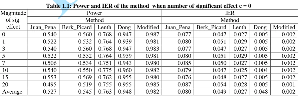
The results obtained from the simulation study are presented in Tables 1.1 to 1.8.

Table 1.1: Power and IER of the method when number of significant effect c = 0 Magnitude

of sig. effect

Power IER

Method Method

(6)

of sig. effect

Power IER

Method Method

Juan_Pena Berk_Picard Lenth Dong Modified Juan_Pena Berk_Picard Lenth Dong Modified 0 0.178 0.272 0.141 0.044 0.016 0.072 0.031 0.018 0.002 0.001 1 0.147 0.225 0.142 0.031 0.014 0.075 0.038 0.019 0.002 0.001 3 0.342 0.453 0.418 0.242 0.106 0.090 0.053 0.033 0.006 0.002 5 0.546 0.645 0.747 0.783 0.382 0.095 0.057 0.038 0.009 0.002 7 0.586 0.678 0.814 0.945 0.694 0.095 0.053 0.033 0.007 0.002 10 0.569 0.658 0.807 0.964 0.941 0.095 0.056 0.034 0.005 0.002 15 0.555 0.652 0.794 0.959 0.985 0.097 0.056 0.036 0.006 0.002 20 0.575 0.634 0.789 0.954 0.991 0.091 0.060 0.037 0.007 0.001 Average 0.437 0.527 0.582 0.615 0.516 0.089 0.051 0.031 0.006 0.002

of sig. effect

Power IER

Method Method

Juan_Pena Berk_Picard Lenth Dong Modified Juan_Pena Berk_Picard Lenth Dong Modified 0 0.102 0.103 0.058 0.008 0.004 0.053 0.018 0.010 0.001 0.000 1 0.110 0.125 0.054 0.009 0.002 0.053 0.016 0.008 0.001 0.000 3 0.249 0.354 0.234 0.106 0.043 0.088 0.039 0.031 0.005 0.001 5 0.566 0.713 0.686 0.677 0.280 0.097 0.056 0.045 0.008 0.003 7 0.640 0.766 0.792 0.949 0.637 0.097 0.051 0.048 0.007 0.003 10 0.624 0.759 0.791 0.969 0.938 0.102 0.053 0.049 0.007 0.002 15 0.644 0.763 0.805 0.975 0.992 0.096 0.053 0.045 0.005 0.002 20 0.640 0.748 0.785 0.963 0.992 0.099 0.055 0.090 0.009 0.002

of sig. effect

Power IER

Method Method

Juan_Pena Berk_Picard Lenth Dong Modified Juan_Pena Berk_Picard Lenth Dong Modified 0 0.074 0.054 0.031 0.001 0.000 0.041 0.006 0.007 - 0.000 1 0.059 0.048 0.027 0.005 0.000 0.042 0.007 0.006 - 0.000 3 0.197 0.237 0.150 0.047 0.017 0.081 0.023 0.027 0.004 0.002 5 0.593 0.753 0.644 0.559 0.219 0.096 0.041 0.053 0.006 0.003 7 0.702 0.865 0.824 0.944 0.597 0.094 0.037 0.049 0.005 0.003 10 0.728 0.880 0.834 0.976 0.927 0.088 0.033 0.050 0.007 0.004 15 0.690 0.861 0.818 0.985 0.991 0.102 0.039 0.054 0.005 0.003 20 0.682 0.855 0.815 0.974 0.995 0.105 0.040 0.055 0.007 0.001

of sig. effect

Power IER

Method Method

(7)

of sig. effect

Power IER

Method Method

Juan_Pena Berk_Picard Lenth Dong Modified Juan_Pena Berk_Picard Lenth Dong Modified 0 0.038 0.007 0.007 0.000 0.000 0.019 0.000 0.001 0.000 0.000 1 0.028 0.007 0.006 0.000 0.000 0.019 0.001 0.002 0.000 0.000 3 0.127 0.061 0.056 0.020 0.006 0.052 0.001 0.010 - 0.001 5 0.602 0.613 0.522 0.325 0.173 0.073 0.007 0.043 0.004 0.003 7 0.786 0.952 0.793 0.849 0.587 0.085 0.010 0.072 0.002 0.003 10 0.808 0.978 0.835 0.993 0.950 0.083 0.009 0.069 0.002 0.001 15 0.783 0.978 0.812 0.990 0.993 0.093 0.009 0.079 0.004 0.003 20 0.824 0.984 0.857 0.992 0.996 0.076 0.006 0.060 0.003 0.002

of sig. effect

Power IER

Method Method

of sig. effect

Power IER

Method Method

4. DISCUSSION OF RESULTS AND CONCLUSIONS

As earlier mentioned, most studies showed that there is no one single method which performs best in all situations. In this study, the proposed method performed best for all values of c and  when IER is used as criteria of assessment. Dong, Lenth, Berkard & Picard and Juan & Pena’s performance follows in the given order with Dong leading. In terms of power, the proposed method performed better than the other at c = 0 and for all values of . However, this proposed method is only better than the other methods for c ≥ 1 and at  ≥ 7. Berk and Picard also performed well in terms of power but it has the disadvantage that it breaks down at large values of c i.e c ≥ 7.

On the overall, combining the two criteria of assessment, the proposed method and Dong are consistent in performance. They have the advantage of

performing in all situations, the proposed method also has the additional advantage of being easy to compute. It is suggested that for future study, situation when the response variable does not follow normal distribution should be explored.

REFERENCES

[AA01] Aboukalam M. A. F., Al-Shiha A. A.

– A Robust Analysis for Unreplicated

Factorial Experiments. Computational Statistical and Data Analysis, 36: 31-46, 2001.

(8)

[AKS12] Angelopoulus P., Koukouvinos C., Skountzou A. – Analysis Method for Unreplicated Factorial Experiments. Springer, New York, 2012.

[Bir59] Birnbaum A. – On the Analysis of

Factorial Experiments without

Replication. Technometrics 1, 343-357, 1959.

[BM86] Box G. E. P., Meyer R. D. – An Analysis for Unreplicated Fractional Factorials, Technometrics, 28, 11-18, 1986.

[BN01] Brenneman W. A., Nair V. N. – Methods of Identifying Dispersion

Effects in Unreplicated Factorial

Experiments: A Critical Analysis and Proposed Strategies. Technometrics, 1, 12-23, 2001.

[BP91] Berk K. N., Picard R. R. –

Significance Tests for Saturated

Orthogonal Arrays, Journal of Quality Technology, 23(2), 79-89, 1991.

[BS06] Bursztyn D., Steinberg D. M. – Screening Experiment for Dispersion Effects methods of Experimentation in Industry, Drug Discovery. Springer Link, New York, 2006.

[BHH78] Box G. E. P., Hunter W. E., Hunter J. S. – Statistics for Experiments. John Wiley, New York, 1978.

[Che03] Chen Y. – On the Analysis of

Unreplicated Factorial Designs.

Unpublished Ph.D. Thesis, 2003. [CP07] Costa N., Pereira Z. L. –

Decision-making in the Analysis of Unreplicated Factorial Designs. Journal of Quality Engineering, 19: 215-225, 2007.

[Dan59] Daniels C. – Uses of Half-Normal Plots in Interpreting Factorial Two-level Experiments. Technometrics, 1, 311-340, 1959.

[Dan76] Daniel C. – Applications of statistics to industrial experimentation, NY: Wiley, 1976.

[Dan94] Danohue J. M. – Experimental Designs for Stimulation. Proceedings of

the Winter Simulation Conference, 200-206, 1994.

[Don93] Dong F. – On the Identification of

Active Contrasts in Unreplicated

Fractional Factorials. Statistica Sinica, 3, 209-217, 1993.

[DV99] Dean A., Voss D. – Design and Analysis of Experiments. Springer, 1999.

[Geo10] George J. B. – Non-linear non-parametric quality screening in low sampling testing. International Journal of Quality and Reliability Management, 27, 893-915, 2010.

[Hoh84] Hohn G. J. – Experimental Design in a Complex World. Technometrics, 26, 19-31, 1984.

[HB88] Hamada M., Balakrishnan N. –

Analyzing Unreplicated Factorial

Experiments: A review with some New Proposals. Statistics Sinica, 8, 1-14, 1988.

[HC95] Haaland P. D., O'Connell M. A. –

Inference for Effect-saturated

Fractional Factorials. Technometrics, 37(1), 82-93, 1995.

[IAO06] Ibraheem B. A., Adeleke B. L., Oyeyemi G. M. – Identification of

Significant Treatment Effects in

Unreplicated Factorial Experiments. BIOMATA, 1, 101-111, 2006.

[JP92] Juan J., Peña D. – A Simple Method to

Identify Significant Effects in

Unreplicated Two-level Factorial

Designs. Communications in Statistics. Theory and Methods, 21(5), 1383-1403, 1992.

[Len89] Lenth R. V. – Quick and Easy Analysis

of Unreplicated Factorials. American Society for Quality, 31, 69-473, 1989. [LN97] Loughin T. M., Noble W. – A

Permutation Test for Effects in an

Unreplicated Factorial Design.

Technometrics, 2, 180-190, 1997. [McG03] McGrath R. N. – Separating Location

(9)

Fractional Factorial Designs. Journal of Quality Technology, 35, 306-316, 2003.

[Mon09] Montgomery D. C. – Design and Analysis of Experiments (7th edn). NJ: John Wiley & Sons, 2009.

[ML01] McGrath R. N., Lin D. K. J. –

Confounding of Location and

Dispersion Effects in Unreplicated

Fractional Factorials. Journal of

Quality Technology, 33, 129-139, 2001.

[Ray67] Rayner A. A. – The Square Summing Check on the main Effects and

Interactions in a 2k Factorial

Experiment as Calculated by Yates’ algorithm. Biometrics, 23: 571-573, 1967.

[ST82] Seheult A., Tukey J. W. – Some

Resistant Procedures for Analyzing 2n

Factorial Experiments. Utilitas Math, 21: 57-98, 1982.

[VW06] Voss D. T., Wang W. – On Adaptive

Testing in Orthogonal Saturated

Designs. Statistica Sinica, 16, 227 – 234, 2006.

[WH00] Wu C. F., Hamada M. – Experiments: Planning, Analysis and Parameter Design Optimization. John Wiley & Sons, 2000.