JIEM, 2016 – 9(3): 634-656 – Online ISSN: 2013-0953 – Print ISSN: 2013-8423 http://dx.doi.org/10.3926/jiem.1703
Comparing Performances of Clements, Box-Cox, Johnson Methods
with Weibull Distributions for Assessing Process Capability
Ozlem Senvar1 , Bahar Sennaroglu2
1Yeditepe University (Turkey) 2Marmara University (Turkey)
[email protected], [email protected]
Received: September 2015
Accepted: June 2016
Abstract:
Purpose: This study examines Clements’ Approach (CA), Box-Cox transformation (BCT), and
Johnson transformation (JT) methods for process capability assessments through Weibull-distributed data with different parameters to figure out the effects of the tail behaviours on process capability and compares their estimation performances in terms of accuracy and precision.
Design/methodology/approach: Usage of process performance index (PPI) Ppu is handled for
process capability analysis (PCA) because the comparison issues are performed through generating Weibull data without subgroups. Box plots, descriptive statistics, the root-mean-square deviation (RMSD), which is used as a measure of error, and a radar chart are utilized all together for evaluating the performances of the methods. In addition, the bias of the estimated values is important as the efficiency measured by the mean square error. In this regard, Relative Bias (RB) and the Relative Root Mean Square Error (RRMSE) are also considered.
Findings: The results reveal that the performance of a method is dependent on its capability to
Research limitations/implications: Some other methods such as Weighted Variance method, which also give good results, were also conducted. However, we later realized that it would be confusing in terms of comparison issues between the methods for consistent interpretations.
Practical implications: Weibull distribution covers a wide class of non-normal processes due to
its capability to yield a variety of distinct curves based on its parameters. Weibull distributions are known to have significantly different tail behaviors, which greatly affects the process capability. In quality and reliability applications, they are widely used for the analyses of failure data in order to understand how items are failing or failures being occurred. Many academicians prefer the estimation of long term variation for process capability calculations although Process Capability Indices (PCIs) Cp and Cpk are widely used in literature. On the other hand, in industry, especially in automotive industry, the PPIs Pp and Ppk are used for the second type of estimations.
Originality/value: Performance comparisons are performed through generating Weibull data
without subgroups and for this reason, process performance indices (PPIs) are executed for computing process capability rather than process capability indices (PCIs). Box plots, descriptive statistics, the root-mean-square deviation (RMSD), which is used as a measure of error, and a radar chart are utilized all together for evaluating the performances of the methods. In addition, the bias of the estimated values is important as the efficiency measured by the mean square error. In this regard, Relative Bias (RB) and the Relative Root Mean Square Error (RRMSE) are also considered. To the best of our knowledge, all these issues including of execution of PPIs are performed all together for the first time in the literature.
Keywords: process performance indices (PPIs), process capability indices (PCIs), process capability
analysis (PCA), non-normal processes
1. Introduction
Principally, process capability can be defined as the ability of the combination of materials, methods, people, machine, equipment, and measurements in order to produce a product that will consistently meet the design requirements or the customer expectations (Kane, 1986). Recent developments in the assessment of process capability have fostered the principle of continuously monitoring and assessing the ability of a process to meet customer requirements (Spiring, 1995).
Álvarez, Moya-Fernández, Blanco-Encomienda and Muñoz (2015) considers process capability analysis (PCA) as a very important aspect in many manufacturing industries. The purpose of PCA involves assessing and quantifying variability before and after the product is released for production, analyzing the variability relative to product specifications, and improving the product design and manufacturing process by reducing the variability. Variation reduction is the key to product improvement and product consistency. For this reason, PCA occupies an important place in manufacturing and quality improvement efforts (Montgomery, 2009).
Process capability index (PCI) is developed to provide a common and easily understood language for quantifying process performance, and is a dimensionless function of process parameters and specifications (Chang, Choi & Bai, 2002). Process capability indices (PCIs) provide numerical measures on whether a process conforms to the defined manufacturing capability prerequisite. In practical aspects, PCIs provide common quantitative measures of the manufacturing capability in terms of production quality to be used by both producer and supplier by means of guidelines when signing a contract. Wang and Du (2007) investigated supply chain performance based on PCI which establishes the relationship between customer specification and actual process performance, providing an exact measure of process yield. Moreover, PCIs have been successfully applied by companies to compete with and to lead high-profit markets by evaluating the quality and productivity performance (Parchamia, Sadeghpour-Gildeha, Nourbakhshb & Mashinchic, 2013).
Hosseinifard, Abbasi and Niaki (2014) also emphasized that conventional methods with a normality assumption fails to provide trustful results. They conduct a simulation study to compare different methods in estimating the process capability index of non-normal processes and then they apply these techniques to obtain the process capability of the leukocyte filtering process.
In literature, several approaches have been proposed to overcome the problems of PCIs for the non-normal distributions. Mathematical transformation of the raw data into approximately non-normal distribution can be an alternative approach that evaluates process capability using the assumption of normality and the transformed data and specification limits. Box-Cox and Johnson's transformations are data transformation techniques. The main aim of all conventional techniques is to use conventional PCIs based on normality assumption. The conventional PCIs can be used once the non-normal data is transformed to normal data. However, practitioners may feel uncomfortable working with transformed data. Reversing the results of the calculations back to the original scale can be troublesome (Pearn & Kotz, 2006). Another way is Clements’ Method which is one of the most popular approaches since it is easy to compute and apply.
Weibull distribution has often been used in the field of lifetime data analysis due to its flexibility, and it can mimic the behaviors of other statistical distributions such as the exponential and gamma. Weibull distributions are used in the analysis of failure data for quality and reliability applications in order to understand how items are failing or failures being occurred. Failures arise from quality deficiencies, design deficiencies, material deficiencies, and so forth. Weibull distribution covers a wide class of non-normal processes due to its capability to yield a variety of distinct curves based on its parameters. The shape parameter of Weibull distribution determines the behavior of the failure rate of the product or system and has been used as a measure of reliability (Yavuz, 2013). Hsu, Pearn and Lu (2011) use Weibull distributions to model the data of the processes and express time until a given technical device fails. They determine the adjustments for capability measurements with the mean shift consideration for Weibull processes. Weibull distributions are known to have significantly different tail behaviours, which greatly affects the process capability. Hosseinifard, Abbasi, Ahmad and Abdollahian (2009) assessed the efficacy of the root transformation technique by conducting a simulation study using gamma, Weibull, and beta distributions. The root transformation technique is used to estimate the PCI for each set of simulated data. They compared their results with the PCI obtained using exact percentiles and the Box-Cox method.
capability rather than PCIs. Box plots, descriptive statistics, the root-mean-square deviation (RMSD), which is used as a measure of error, and a radar chart are utilized all together for evaluating the performances of the methods. To the best of our knowledge, all these issues including of execution of PPIs are performed all together for the first time in the literature.
The rest of the paper is organized as follows: In section 2, PCIs with short term and long term variation within PCA are given. In Section 3, Clements’, Box-Cox, Johnson transformation methods are explained. In Section 4, these methods are applied to Weibull distributions to examine the impact of non-normal data on the process performance index Ppu. In Section 5, the results are given, and comparisons are made according to the results. The last section provides concluding remarks and recommendations.
2. Process Capability Analysis (PCA)
Process capability deals with the uniformity of the process. Variability of critical to quality characteristics in the process is a measure of the uniformity of outputs. Here, variability can be thought in two ways: one is inherent variability in a critical to quality characteristic at a specified time, and the other is variability in a critical to quality characteristic over time (Montgomery, 2009). Process capability compares inherent variability in a process with the specifications that are determined according to the customer requirements. In other words, process capability is the proportion of actual process spread to the allowable process spread, which is measured by six process standard deviation units. Principally, process capability is the long term performance level of the process after it has been brought under statistical control.
PCA involves statistical techniques (Senvar & Tozan, 2010). PCA is used to estimate the process capability and evaluate how well the process will hold the customer tolerance. PCA can be useful in selecting or modifying the process during product design and development, selecting the process requirements for machines and equipment, and reducing the variability in production processes.
In assessing process capability, both short term and long term PCIs are computed and are not considered separately. Different real (targeted) indices (Ppu, Cp, Cpk, Pp, Ppk, etc) can be used. The Cp and Cpk are short term PCIs and are computed using short term standard deviation. On the other hand, Pp and Ppk are long term PPIs and are computed using long term standard deviation estimate.
The sigma quality level of a process can be used to express its capability that means how well it performs with respect to specifications. As a measure of process capability, it is customary to take six sigma spread in the distribution of product quality characteristic.
For a process whose quality characteristic x has a normal distribution with process mean μ and process standard deviation σ; the lower natural tolerance limit of the process is LNTL = μ – 3σ, and the upper natural tolerance limit of the process is UNTL = μ + 3σ. It should be considered that natural tolerance limits include 99.73% of the variable and 0.27% of the process output falls outside the natural tolerance limits.
The standard assumptions in statistical process control (SPC) are that the observed process values are normally, independently and identically distributed (IID) with fixed mean μ and standard deviation σ when the process is in control. Due to the dynamic behavior, these assumptions are not always valid. The data may not be normally distributed and/or autocorrelated, especially when the data are observed sequentially and the time between samples is short (Haridy & Wu, 2009). Statistical analysis of non-normal data is usually more complicated than that for non-normal distribution (Abbasi, 2009). It is always crucial to estimate PCI when the quality characteristic does not follow normal distribution, however skewed distributions come about in many processes. The classical method to estimate process capability is not applicable for non-normal processes. In the existing methods for non-normal processes, probability density function (pdf) of the process or an estimate of it is required. Estimating pdf of the process is a hard work and resulted PCI by estimated pdf may be far from real value of it. Abbasi (2009) proposed an artificial neural network to estimate PCI for right skewed distributions without appeal to pdf of the process.
When data follows a well-known, but non-normal distribution, such as Weibull distribution, computation of defect rates is performed by using the properties of the distribution given the parameters of the distribution and the specification limits. Besseris (2014) performed interpretation of key indices from a non-parametric viewpoint and recommended method for estimating PCIs as purely distribution-free, and deployable at any process maturity level.
3. Clements’, Box-Cox, Johnson Transformation Methods
When the distribution of a process characteristic is non-normal, conventional methods give erroneous interpretation of process capability. For computing PCIs under non-normality, various methods have been proposed in the literature. Tang, Than and Ang (2006) classified these methods into two main categories as transformation and non-transformation methods. Transformation methods are Box-Cox power transformation, Johnson transformation system, Clements’ method using Pearson curves. Non-transformation methods are Wright’s index, Probability plot, Weighted variance method. In this study, we will focus on Clements’ method and both Box-Cox and Johnson transformation methods.
3.1. Transformation Methods
Kane (1986) suggested transforming data for maintaining an approximately normal distribution. Among various researchers and applied statisticians, Gunter (1989) empirically proved that the results of transformed data are much better than the results of the original raw data. Generally, transformations are used for three purposes:
1. Stabilising response variance
2. Making distribution of the response variable closer to the normal
3. Improving the fit of the model to the data including model simplification, i.e. by eliminating interaction terms.
transformation methods because of the problems associated with translating the computed results with regard to the original scales (Kotz & Johnson, 2002; Ding, 2004).
Most known amongst these methods are Box-Cox power transformation based on maximization of a log-likelihood function and Johnson transformation system based on derivation of the moments of the distribution. Yeo and Johnson (2000) introduced a new power transformation family which is well defined on the whole real line and which is appropriate for reducing skewness and to approximate normality. They provided desirable properties, such as the fact it can be used for both negative and positive values. It has properties similar to those of the Box-Cox transformation for positive variables. The larges ample properties of the transformation are investigated in the contect of a single random sample.
In this study, we handled Box-Cox power transformation and Johnson transformation in the following context:
3.1.1. Box-Cox power Transformation (BCT)
The Box-Cox transformation was proposed by Box and Cox in 1964 and used for transforming non-normal data (Box & Cox, 1964). The Box-Cox transformation uses the parameter λ. In order to transform the data as closely as possible to normality, the best possible transformation should be performed by selecting the most appropriate value of λ. In order to obtain the optimal λ value, Box-Cox transformation method requires maximization of a log-likelihood function. After the transformation, process capability can be evaluated.
Box & Cox (1964) proposed a useful family of power transformations on the necessarily positive response variable X. The Box-Cox power transformation is given in Equation 1.
(1)
where variable X necessarily takes positive values. In other words, Box-Cox transformation can be done only on non-zero, positive data. If there are negative values, a constant value can be added in order to make the values positive. This continuous family depends on a single parameter λ that can be estimated by using maximum likelihood estimation. Firstly, a value of λ from a pre-assigned range is collected. Then,
(2)
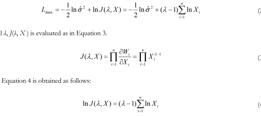
For all λ, J(λ, X ) is evaluated as in Equation 3.
(3)
Thus, Equation 4 is obtained as follows:
(4)
For fixed λ, σ2 is estimated by using S(λ), which is the residual sum of squares of X (λ). σ2 is estimated by the formula in Equation 5.
(5)
When the optimum value of λ is obtained, for all the quality characteristic values of X, upper and lower specification limits are transformed to normal variables (Yang, Song & Ming, 2010). Therefore, the corresponding PCIs, Cp and Cpk, can be computed from the mean and standard deviation of the transformed data just like computations of Cp and Cpk under normality. Box-Cox transformation is best done using computers. Most statistical software packages offer Box-Cox transformation as a standard feature.
3.1.2. Jonhson Transformation System Using Pearson Curves (JT)
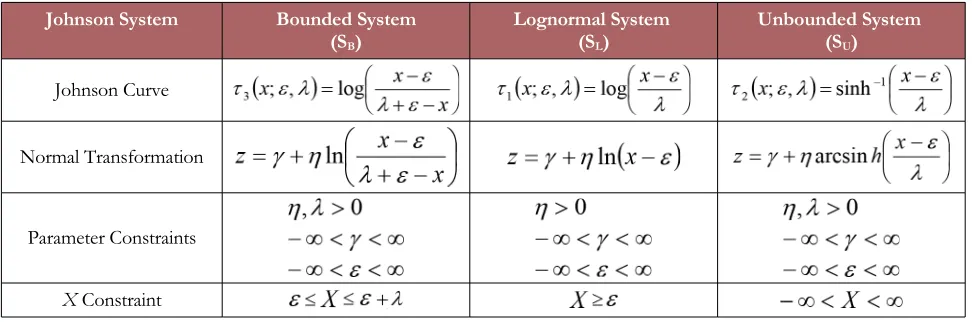
Johnson (1949) proposed a system of distributions, which is called the Johnson transformation system based on the moment method. Simply, Johnson method requires fitting of the first four moments in order to determine the appropriate Johnson family. Process capability can be evaluated after selecting the optimal transform function in which transformed data comes closest to normality. Johnson transformation internally evaluates several transform functions and optimally selects one, which transforms the data closest to the normality, from three families of distributions, which transform the data into a normal distribution. These three distributions are lognormal, unbounded, and bounded.
Step 1. Select a suitable z.
Step 2. Find the probability distribution p-sz, p-z, pz and psz corresponding to {-sz, -z, z, sz} Step 3. Find the corresponding quantile x-sz, x-z, xz, xsz in the sample data.
Step 4. Let m = xsz -xz, η = x-z, x-sz, p = xz x-z Step 5. Define the quantile ratio (QR) as
Bounded System (SB) and Unbounded System (SU) can be selected according to the following general condition:
If 1 < s ≤ 3 and OR < (s – 1)2/4, then select SB
If s ≥ 3 and OR > (s – 1)2/4, then select SU
When s = 3, the rule is determined to differentiate among Bounded System (SB), Lognormal System (SL), and Unbounded System (SU).
When QR < 1, select Bounded System (SB). When QR = 1, select Lognormal System (SL). When QR > 1, select Unbounded System (SU).
Johnson System Bounded System (SB)
Lognormal System (SL)
Unbounded System (SU)
Johnson Curve
Normal Transformation
Parameter Constraints
X Constraint
Table 1. Summary of Johnson transformation system (Yang et al., 2010)
probabilities 0.00135, 0.5 and 0.99865 can be obtained. Hence, the corresponding process capability index can be evaluated (Yang et al., 2010).
3.2. Clements Approach
The well-known quantile estimation techniques were developed by Clements (1989), who utilized the Pearson curves to provide better estimates of the relevant quantiles. Non-normal Pearsonian distributions include a wide class of populations with non-normal characteristics. This method uses Pearson curves to provide more accurate estimates of x0.00135, x0.50 (median), and x0.99865. Modified Cp and Cpk do not require transformation of the data and they have straightforward meaning which makes them easy to understand. Also, their estimations are fairly easy to be computed (Pearn & Kotz, 2006).
Clements’ estimator for Cp (Equation 6) is obtained by replacing 6σ by subtracting x0.00135 from x0.99865
(x0.99865 – x0.00135) and for Cpk (Equation 7) by replacing the mean µ by the median x0.50. Notably, x0.99865is the 0.99865 quantile, x0.00135 is the 0.00135 quantile, and x0.50 is the 0.50 quantile calculated with the knowledge of skewness, kurtosis, mean, and variance from the sample data for a non-normal Personian distribution. In Equations 6 and 7, USL and LSL denote upper specification limit and lower specification limit, respectively.
(6)
(7)
4. Sample and Methods
In this study, Weibull distributions are executed to examine the impact of non-normal data on the PPI
Ppu. Computations are performed by using Minitab 16 and MS Excel 2010 as software packages.
The cumulative distribution function (CDF) of a Weibull distribution having shape parameter α and scale parameter β is expressed as in Equation 8.
Weibull Distributions with shape and scale parameters of (1,1), (1,2), (2,1), and (2,2) are considered in the simulation study. 50 data sets (r = 50) are randomly generated by sample size of 100 (n=100) from Weibull (1,1), (1,2), (2,1), and (2,2), respectively. Notice that, first two Weibull distributions with their shape parameter values of 1 are at the same time Exponential distributions. Because when its shape parameter is equal to 1, the Weibull distribution reduces to the Exponential distribution with its parameter equal to the reciprocal of the scale parameter of the Weibull distribution.
USL is calculated through Equation 9 using the targeted capability index values of 1.0 and 1.5 for quantile-based process capability index Cpu(q) by considering theoretical distribution with the specified parameters.
(9)
where USL denotes upper specification limit, and x0.99865 and x0.50 (median) correspond to 0.99865 and 0.50 cumulative probabilities of the distribution, respectively. When a transformation method is used, USL is transformed by the corresponding transformation formula.
Table 2 illustrates the corresponding quantiles, mean, median along with skewness and kurtosis based on the specified parameter values of Weibull distribution for this study. It is interesting to observe the difference between the mean and the median for the different distributions. Kurtosis gives information about the relative concentration of values in the center of the distribution as compared to the tails. Data sets with high kurtosis tend to have prominent peak and heavy tails. Skewness gives information about whether the distribution of the data is symmetrical. The skewness for a normal distribution is zero. The positive skewness values indicate that the distribution is positively skewed, which corresponds that right tail is longer than the left tail, and for negative skewness values it is vice versa. Therefore, it can be stated that kurtosis and skewness give information about tail behavior of a distribution.
Weibull (α,β ) x0.99865 Median = x0.50 Mean Skewness Kurtosis
Weibull (1,1) 6.607650 0.693147 1 1.676698 3.413711
Weibull (1,2) 13.215300 1.386290 2 1.747334 3.982865
Weibull (2,1) 2.570540 0.832555 0.7071 0.562298 0.104820
Weibull (2,2) 5.141070 1.665110 1.4142 0.590805 0.212021
The probability density functions (PDFs) of these distributions are plotted in Figure 1. The average values of skewness and kurtosis calculated from 50 data sets (r = 50) each having sample size of 100 observations (n = 100) are generated randomly for each Weibull distribution with specified parameters.
Figure 1. PDFs of Weibull distributions
For the skewed processes, the proportion of nonconforming items for fixed values of standard PCIs tends to increase as skewness increases. For instance, the standard PCIs simply ignore the skewness of the underlying population. For example; if the underlying distribution is Weibull with the shape parameter (α = 2.0), the skewness is 0.63 or Weibull distribution with the shape parameter (α = 1.0), the skewness is 2.00. Then the expected proportions of non-conforming items below and above the LSL = –3.0 and USL = 3.0 are 0.56% and 1.83%, respectively, for the same value of μ = 0 and σ = 1. Hence Cp = Cpk = 1.0, whereas the expected non-conforming proportion for a normal population is 0.27% (Pearn and Kotz, 2006). As a matter of fact, it is very desirable to consider the skewness of the underlying population by a method of adjusting the values of a PCI in accordance with the expected proportion of non-conforming items.
In this study, the Weibull data are generated without subgroups, therefore, PPI Ppu is used for PCA. Ppu is the ratio of the interval formed by the process mean and USL to one-sided spread of the process and is estimated using Equation 10.
(10)
(11)
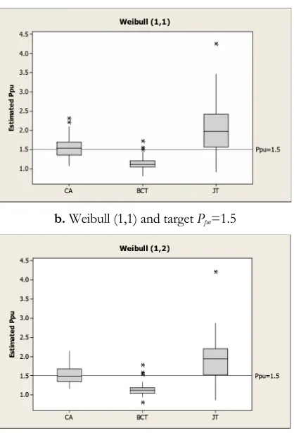
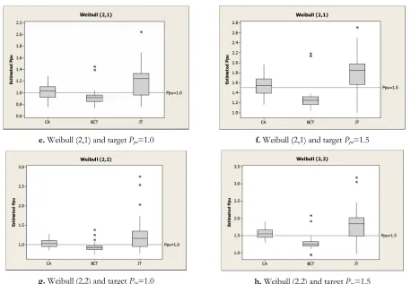
Firstly, we figured out box plots in order to compare the transformation methods graphically at each targeted Ppu (1.0 and 1.5). A box plot (also known as box and whisker plot) is used to show the shape of the distribution, its central value (x0.50), variability (x0.75 – x0.25), and outliers by star symbol if exist. The position of the median line in a box plot indicates the location of the values.
Figure 2 shows box plots with targeted Ppu values of 1.0 and 1.5. According to Figure 2 CA provides the most accurate estimates in comparison to the other methods. While, BCT underestimates the targeted values, JT overestimates them. Overestimation and underestimation of the targeted values point out less accuracy for the methods.
a. Weibull (1,1) and target Ppu=1.0 b. Weibull (1,1) and target Ppu=1.5
e. Weibull (2,1) and target Ppu=1.0 f. Weibull (2,1) and target Ppu=1.5
g. Weibull (2,2) and target Ppu=1.0 h. Weibull (2,2) and target Ppu=1.5
Figure 2. Box plots of CA, BCT, and JT methods
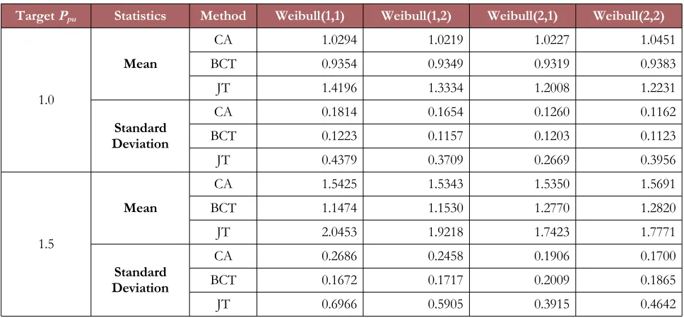
Target Ppu Statistics Method Weibull(1,1) Weibull(1,2) Weibull(2,1) Weibull(2,2)
1.0
Mean
CA 1.0294 1.0219 1.0227 1.0451
BCT 0.9354 0.9349 0.9319 0.9383
JT 1.4196 1.3334 1.2008 1.2231
Standard Deviation
CA 0.1814 0.1654 0.1260 0.1162
BCT 0.1223 0.1157 0.1203 0.1123
JT 0.4379 0.3709 0.2669 0.3956
1.5
Mean
CA 1.5425 1.5343 1.5350 1.5691
BCT 1.1474 1.1530 1.2770 1.2820
JT 2.0453 1.9218 1.7423 1.7771
Standard Deviation
CA 0.2686 0.2458 0.1906 0.1700
BCT 0.1672 0.1717 0.2009 0.1865
JT 0.6966 0.5905 0.3915 0.4642
Table 3. Descriptive statistics for CA, BCT, and JT methods
Using the formula in Equation 12, the root-mean-square deviation (RMSD) is used to measure the differences between the target Ppu values and the estimates obtained by CA, BCT, and JT methods.
(12)
where r is the number of data sets generated randomly for each Weibull distribution with specified parameters. Notice that, 50 data sets (r = 50) each having sample size of 100 observations (n = 100) are generated randomly for each Weibull distribution with Weibull Distributions with shape and scale parameters of (1,1), (1,2), (2,1), and (2,2) are considered in the simulation study. In other words, 50 data sets (r=50) are randomly generated by sample size of 100 (n = 100) from Weibull (1,1), (1,2), (2,1) and (2,2), respectively.
Target Ppu Method Weibull (1,1) Weibull (1,2) Weibull (2,1) Weibull (2,2)
1.0
CA 0.18 0.17 0.13 0.12
BCT 0.14 0.13 0.14 0.13
JT 0.60 0.50 0.33 0.45
1.5
CA 0.27 0.25 0.19 0.18
BCT 0.39 0.39 0.30 0.29
JT 0.88 0.72 0.46 0.54
Table 4. The root-mean-square deviations for CA, BCT, and JT methods
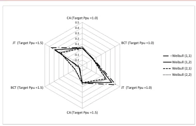
The Weibull distributions (1,1) and (1,2) with near values of skewness and kurtosis (Table 2) have similar tail behaviors and as it can be observed in Figure 3 that shows radar chart. All methods produce high RMSD values for these distributions. It is also observed that the RMSD values for Weibull distributions (1,1) and (1,2) are higher at the target Ppu of 1.5 than that of 1.0 for all methods. This result indicates that the effect of tail behavior is more significant when the process is more capable.
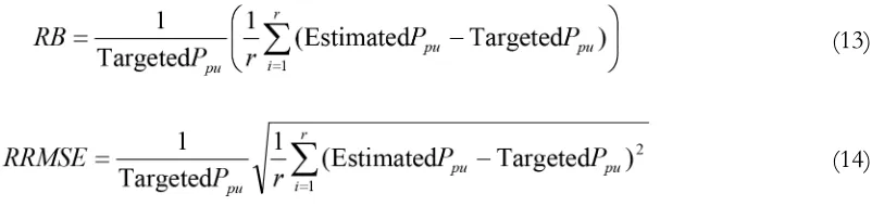
It has to be emphasized that some scientists discuss that RMSD is not a good measure to compare the different Weibull distributions, since the RMSD is not a relative measure. In addition, the bias of the estimated values is important as the efficiency measured by the mean square error. In this regard, Relative Bias (RB) (Equation 13) and the Relative Root Mean Square Error (RRMSE) (Equation 14) can also be considered. These measures are defined by Chambers and Dunstan (1986), Rao Kovar and Mantel (1990), Silva and Skinner (1995), Muñoz and Rueda (2009), etc.
(13)
(14)
Figure 3. Radar Chart for RB
5. Discussion and Conclusion
PCA occupies an important place in manufacturing environment. PCIs are used to define the relationship between technical specifications and production abilities which lead to operational decisions about manufacturing and purchasing.
In industrial practices, a variety of processes result in a non-normal distribution for a quality characteristic. In this case, PCIs become sensitive to departures from normality. When the distribution of a process characteristic is non-normal, PCIs computed by conventional methods would give unreliable, misleading results as well as erroneous or incorrect interpretations of process capability. Incorrect application or interpretation of the PCIs causes unreliable results, which can lead incorrect decision making, waste of resources, money, time, and etc.
In manufacturing environment, Weibull-distributed quality characteristics are encountered a lot, especially when controlling the process components in terms of times-to-failure. Weibull distributions are known to have significantly different tail behaviours, which greatly affects the process capability. In order to examine the impact of non-normal data, the parameter values of Weibull distribution are specified as (1,1), (1,2), (2,1), and (2,2) corresponding to (shape, scale). These parameters of Weibull distributions are specified such that the effects of the tail behaviours on process capability could be examined. Principally, when its shape parameter is equal to 1, Weibull distribution reduces to Exponential distribution. Hence, this study covers Exponential distribution, as well.
The comparison is performed through generating Weibull data without subgroups and therefore, Ppu is used in PCA in this study. Many academicians prefer the estimation of long term variation for process capability calculations although Cp and Cpk is widely used in literature. On the other hand, in industry, especially in automotive industry, the Pp and Ppk notations are used for the second type of estimations.
This study examines three methods (CA, BCT, JT) for process capability through Weibull-distributed data with different parameters and compares their estimation performances in term of accuracy and precision. Performance comparison of methods is made in terms of box plots, descriptive statistics, the root-mean-square deviation, and a radar chart. In addition, the bias of the estimated values is important as the efficiency measured by the mean square error. In this regard, Relative Bias (RB) and the Relative Root Mean Square Error (RRMSE) are also considered.
taken into account that a method that performs well for a particular distribution may give erroneous results for another distribution with a different tail behaviour. It is observed in this study that the effect of tail behavior is more significant when the process is more capable.
For further directions, inducing some of the new methods such as Best Root Transformation method into the comparison. For recommendations, we emphasize that all methods should be employed with same índices. We tried to execute Weighted Variance method that provides good results. However, we did not involve in this study because we later realized that it would be confusing in terms of comparison issues between the methods for consistent interpretations.
We believe that our findings would be helpful for selecting appropriate methods in process capability assessments with non-normal processes, especially with Weibull or Exponentially distributed quality characteristic. It is possible to conclude that since Weibull distribution has relationships with the other distributions, such as Exponential and Normal distribution, this study can also be a guideline for the other non-normal processes for further directions. It should be emphasized that our understanding of distributions that provide good models for most non-normal data of quality and process characteristics, are the Weibull, Log-normal, and Exponential distributions that have been extensively used in quality and reliability applications.
References
Abbasi, B. (2009). A neural network applied to estimate process capability of non-normal processes. Expert Systems with Applications, 36(2), 3093-3100. http://dx.doi.org/10.1016/j.eswa.2008.01.042
Álvarez, E., Moya-Fernández, P.J., Blanco-Encomienda, F.J., & Muñoz, J.F. (2015). Methodological insights for industrial quality control management: The impact of various estimators of the standard deviation on the process capability index. Journal of King Saud University–Science. In press. http://dx.doi.org/10.1016/j.jksus.2015.02.002
Besseris, G. (2014). Robust process capability performance: An interpretation of key indices from a nonparametric viewpoint. The TQM Journal, 26(5), 445-462. http://dx.doi.org/10.1108/TQM-03-2013-0036 Box, G.E.P., & Cox, D.R. (1964). An analysis of transformations. Journal of the Royal Statistical Society: Series
B, 26, 211-252.
Chambers, R.L., & Dunstan, R. (1986). Estimating distribution functions from survey data. Biometrika, 73, 597-604. http://dx.doi.org/10.1093/biomet/73.3.597
Chang, Y.S., Choi, I.S., & Bai, D.S. (2002), Process capability indices for skewed populations. Quality and Reliability Engineering International, 18(5), 383-393. http://dx.doi.org/10.1002/qre.489
Clements, J.A. (1989), Process capability indices for non-normal calculations. Quality Progress, 22, 49-55.
Ding, J. (2004). A method of estimating the process capability index from the first moments of non-normal data. Quality and Reliability Engineering International, 20(8), 787-805.
http://dx.doi.org/10.1002/qre.610
Gunter, B.H. (1989). The use and abuse of Cpk: Parts 1-4. Quality Progress, 22(1), 72-73; 22(3), 108-109; 22(5), 79-80 and 22(7), 86-87.
Haridy, S., & Wu, Z. (2009). Univariate and multivariate control charts for monitoring dynamic-behavior processes: A case study. Journal of Industrial Engineering and Management, 2(3), 464-498. http://dx.doi.org/10.3926/jiem.2009.v2n3.p464-498
Hosseinifard, S.Z., Abbasi, B., Ahmad, S., & Abdollahian, M. (2009). A transformation technique to estimate the process capability index for non-normal processes. The International Journal of Advanced Manufacturing Technology, 40(5), 512-517. http://dx.doi.org/10.1007/s00170-008-1376-x
Hosseinifard, S.Z, Abbasi, B., & Niaki, S.T.A. (2014). Process capability estimation for leukocyte filtering process in blood service: A comparison study. IIE Transactions on Healthcare Systems Engineering, 4(4), 167-177. http://dx.doi.org/10.1080/19488300.2014.965393
Hsu, Y.C., Pearn, W.L., & Lu, C.S. (2011). Capability measures for Weibull processes with mean shift based on Erto’s-Weibull control chart. International Journal of Physical Sciences, 6(19), 4533-4547.
Johnson, N.L. (1949). Systems of frequency curves generated by methods of translation. Biometrika, 36, 149-176. http://dx.doi.org/10.1093/biomet/36.1-2.149
Kane, V.E. (1986). Process capability indices. Journal of Quality Technology, 18, 41-52.
Kotz, S., & Johnson, N.L. (2002). Process capability indices – a review, 1992-2000 (with subsequent discussions and response). Journal of Quality Technology, 34(1), 2-53.
Montgomery, D.C. (2009). Statistical Quality Control: A Modern Introduction, 6th edition. New York: Wiley. Muñoz, J.F., & Rueda, M.M. (2009). New imputation methods for missing dada using quantiles. Journal of
Computational and Applied Mathematics, 232, 305-317. http://dx.doi.org/10.1016/j.cam.2009.06.011
Parchamia, A., Sadeghpour-Gildeha, B., Nourbakhshb, M. & Mashinchic, M. (2013). A new generation of process capability indices based on fuzzy measurements. Journal of Applied Statistics, 41(5), 1122-1136. http://dx.doi.org/10.1080/02664763.2013.862219
Pearn, W.L., & Kotz, S. (2006). Encyclopedia and Handbook of Process Capability Indices: A Comprehensive Exposition of Quality Control Measures. Singapore: World Scientific Publishing Company. http://dx.doi.org/10.1142/6092
Rao, J.N.K., Kovar, J.G., & Mantel, H.J. (1990). On estimating distribution function and quantiles from survey data using auxiliary information. Biometrika, 77, 365-375. http://dx.doi.org/10.1093/biomet/77.2.365 Senvar, O., & Kahraman, C. (2014a). Fuzzy process capability indices using clements' method for
non-normal processes. Journal of Multiple-Valued Logic and Soft Computing, 22(1-2), 95-121. ISSN: 15423980.
Senvar, O., & Kahraman, C. (2014b). Type-2 fuzzy process capability indices for nonnormal processes.
Journal of Intelligent and Fuzzy Systems, 27(2), 769-781.http://dx.doi.org/10.3233/IFS-131035
Senvar, O., & Tozan, H. (2010). Process Capability and Six Sigma Methodology Including Fuzzy and Lean Approaches. In Fuerstner, I. (Ed.). Products and Services; from R&D to Final Solutions, Chapter 9, InTech. 154-179. http://dx.doi.org/10.5772/10389
Silva, P.L.D., & Skinner, C.J. (1995). Estimating distribution function with auxiliary information using poststratification. Journal of Official Statistics, 11, 277-294.
Spiring, F.A. (1995). Process capability: A total quality management tool. Total Quality Management, 6(1), 21-34. http://dx.doi.org/10.1080/09544129550035558
Tang, L.C., & Than, S.E. (1999). Computing process capability indices for non-normal data: A review and comparative study. Quality and Reliability Engineering International, 15, 339-353. http://dx.doi.org/10.1002/ (SICI)1099-1638(199909/10)15:5<339::AID-QRE259>3.0.CO;2-A
Wang, F.-K., & Du, T. (2007). Applying Capability Index to the Supply Network Analysis. Total Quality Management & Business Excellence, 18(4), 425-434. http://dx.doi.org/10.1080/14783360701231807
Yang, J.R., Song, X.D., & Ming, Z. (2010). Comparison between Nonnormal Process Capability Study Based on Two Kinds of Transformations. Proceedings of the First ACIS International Symposium on Cryptography, and Network Security, Data Mining and Knowledge Discovery, E-Commerce and Its Applications, and Embedded Systems. Qinhuangdao, Hebei, China, 332-336. http://dx.doi.org/10.1109/cdee.2010.103
Yavuz, A.A. (2013). Estimation of the Shape Parameter of the Weibull Distribution Using Linear Regression Methods: Non-Censored Samples. Quality and Reliability Engineering International, 29, 1207-1219. http://dx.doi.org/10.1002/qre.1472
Yeo, I.K., & Johnson, R.A. (2000). A new family of power transformations to improve normality or symmetry. Biometrika, 87, 954-959. http://dx.doi.org/10.1093/biomet/87.4.954
Journal of Industrial Engineering and Management, 2016 (www.jiem.org)
Article's contents are provided on an Attribution-Non Commercial 3.0 Creative commons license. Readers are allowed to copy, distribute and communicate article's contents, provided the author's and Journal of Industrial Engineering and Management's