Isolated-word speech recognition using hidden Markov models
H˚akon Sandsmark
December 18, 2010
1
Introduction
Speech recognition is a challenging problem on which much work has been done the last decades. Some of the most successful results have been obtained by using hidden Markov models as explained by Rabiner in 1989 [1].
A well working generic speech recognizer would enable more efficient communication for everybody, but especially for children, analphabets and people with disabilities. A speech recognizer could also be a subsystem in a speech-to-speech translator.
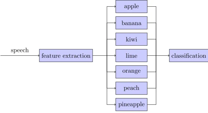
The speech recognition system implemented during this project trains one hidden Markov model for each word that it should be able to recognize. The models are trained with labeled training data, and the classification is performed by passing the features to each model and then selecting the best match.
feature extraction
apple
banana
kiwi
lime
orange
peach
pineapple
[image:1.595.117.477.417.613.2]classification speech
2
Background theory
2.1 Hidden Markov models
Basic knowledge of hidden Markov models is assumed, but the two most important algorithms used in this project will be described.
The observable output from a hidden state is assumed to be generated by a mul-tivariate Gaussian distribution, so there is one mean vector and covariance matrix for each state. We will also assume that the state transition probabilities are independent of time, such that the hidden Markov chain is homogenous.
We will now define the notation for describing a hidden Markov model as used in this project. There is a total number of N states. An element ass0 in the transition
probability matrix A denotes the transition probability from state s to state s0, and the probability for the chain to start in state s is πs. The mean vector and covariance
matrix for the multivariate Gaussian distribution modeling the observable output from statesare µs and Σs, respectively. For an observationo,bs(o) denotes the probability
density of the multivariate Gaussian distribution of state s at the values ofo. We will sometimes denote the collection of parameters describing the hidden Markov model as
λ={A, π, µ,Σ}.
2.2 The forward algorithm
We want to calculate the probability density of an observation o1, . . . ,oT for a specific
model. This will be used to select the model (i.e. word) that most likely generated the speech signal.
f(o1, . . . ,oT;λ) =
X
sT
f(o1, . . . ,oT, sT;λ) (1)
=X
sT
f(oT|o1, . . . ,oT−1, sT;λ)f(o1, . . . ,oT−1, sT;λ) (2)
=X
sT
bsT(oT) X
sT−1
f(o1, . . . ,oT−1, sT−1, sT;λ) (3)
=X
sT
bsT(oT) X
sT−1
f(sT|o1, . . . ,oT−1, sT−1;λ)f(o1, . . . ,oT−1, sT−1;λ)
(4)
=X
sT
bsT(oT) X
sT−1
asT−1sTf(o1, . . . ,oT−1, sT−1;λ) (5)
The recursive structure is revealed as we reduced the problem from needingf(o1, . . . ,oT, sT;λ)
for all sT to needingf(o1, . . . ,oT−1, sT−1;λ) for all sT−1. Let us introduce the forward
α1(s)≡f(o1, S1=s;λ) (6)
=bs(o1)πs (7)
αt(s)≡f(o1, . . . ,ot, St=s;λ) (8)
=bs(ot)
X
s0
as0sαt−1(s0) (9)
Then our solution can be expressed nicely as
f(o1, . . . ,oT;λ) =
X
s
αT(s). (10)
Implemented na¨ıvely top-down (backwards in time) this would not bring us any luck because of the exponentially recursive structure. The na¨ıve algorithm is however easily convertible to an efficient variant using dynamic programming where we calculate the forward variables bottom-up (forwards in time). We simply calculateαt(s) for all states s, first fort= 1 and then all the way up toT. This way all the forward variables from the previous time step are readily available when needed.
2.3 The Baum-Welch algorithm
We want to find the parametersλthat maximize the likelihood of the observations. This will be used to train the hidden Markov model with speech signals. The Baum-Welch algorithm is an iterative expectation-maximization (EM) algorithm that converges to a locally optimal solution from the initialization values.
The M-step consists of updating the parameters in the following intuitive way:
πs :=πs=
expected number of times in statesatt= 1
expected number of times att= 1 (11)
ass0 :=ass0 = expected number of transitions fromstos
0
expected number of transitions froms (12)
µs :=µs= expected observation when in state s (13)
Σs :=Σs= observation covariance when in states (14)
The E-step thus consists of calculating these expectations for a fixed λ. Let Vs(t)
denote the event of transition from statesat time stept, andVs,s(t)0 the event of transition
πs=E{1[Vs(1)]}=P(Vs(1)) (15)
ass0 =
E{Pt1[V
(t)
s,s0]}
E{Pt1[V
(t)
s ]}
=
P
tP(V
(t)
s,s0)
P
tP(V
(t)
s )
(16)
µs= E
{P
t1[V
(t)
s ]ot}
E{Pt1[V
(t)
s ]}
=
P
tP(V
(t)
s )ot
P
tP(V
(t)
s )
(17)
Σs= E
{P
t1[V
(t)
s ](otoTt −µsµsT)}
E{Pt1[V
(t)
s ]}
=
P
tP(V
(t)
s )otoTt
P
tP(V
(t)
s )
−µsµsT (18)
Note that the non-italic T denotes transpose and has nothing to do with time. To be able to calculate these probabilities we first introduce the backward variable which is very similar to the forward variable previously defined.
βT(s)≡1 (19)
βt(s)≡f(ot+1, . . . ,oT|St=s;λ) (20)
=X
s0
ass0bs0(ot+1)βt+1(s0) (21)
The backward variable has its name because it is first calculated for the last time step and then backwards in time when implemented with dynamic programming (essentially the reverse procedure of the one described in detail for the forward variable).
Then we rename the probabilities to the same symbols as used by Rabiner and express them by forward and backward variables:
γt(s)≡P(Vs(t)) =P(St=s|o1, . . . ,oT;λ) (22)
= f(o1, . . . ,oT|St=s)P(St=s)
f(o1, . . . ,oT)
(23)
= f(o1, . . . ,ot, St=s)f(ot+1, . . . ,oT|St=s)
f(o1, . . . ,oT)
(24)
= αt(s)βt(s)
f(o1, . . . ,oT)
(25)
And similarly (details omitted):
ξt(s, s0)≡P(Vs,s(t)0) =P(St=s, St+1 =s0|o1, . . . ,oT;λ) (26)
= αt(s)bs0(ot+1)ass0βt+1(s
0)
f(o1, . . . ,oT)
(27)
πs =γ1(s) (28)
ass0 =
P
tξt(s, s0)
P
tγt(s)
(29)
µs =
P
tγt(s)ot
P
tγt(s)
(30)
Σs =
P
tγt(s)otoTt
P
tγt(s)
−µsµsT (31)
To summarize the E-step boils down to computing γt(s) and ξt(s, s0) for all s, s0
and twhile the parametersλare fixed, and then the M-step will updateλby using the calculations done in the E-step. This is iterated until satisfaction.
3
System design
3.1 Feature extraction
The source speech is sampled at 8000 Hz and quantized with 16 bits. The signal is split up in short frames of 80 samples corresponding to 10 ms of speech. The frames overlap with 20 samples on each side. The idea is that the speech is close to stationary during this short period of time because of the relatively limited flexibility of the throat. We will pick out our features from the frequency domain, but before we get there by taking the fast Fourier transform, we multiply by a Hamming window to reduce spectral leakage caused by the framing of the signal.
0 10 20 30 40 50 60 70 80
ï1
ï0.8
ï0.6
ï0.4
ï0.2 0 0.2 0.4 0.6 0.8 1
time
Speech signal Hamming window
(a) Speech signal and Hamming window in time domain.
0 500 1000 1500 2000 2500 3000 3500 4000 0
0.5 1 1.5 2 2.5 3 3.5x 10
ï3
F [Hz]
|X(F)|
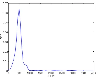
[image:5.595.324.483.433.561.2](b) Single-sided magnitude spectrum of the same speech signal multiplied by the Hamming window.
Figure 2: An 80 sample frame of an unvoiced part of a speech signal. Unvoiced speech, like ‘sh’, is more noisy and contains higher frequencies than voiced speech.
0 10 20 30 40 50 60 70 80 ï1
ï0.8 ï0.6 ï0.4 ï0.2 0 0.2 0.4 0.6 0.8 1
time
Speech signal Hamming window
(a) Speech signal and Hamming window in time domain.
0 500 1000 1500 2000 2500 3000 3500 4000
0 0.01 0.02 0.03 0.04 0.05 0.06 0.07
F [Hz]
|X(F)|
[image:6.595.322.482.111.239.2](b) Single-sided magnitude spectrum of the same speech signal multiplied by the Hamming window.
Figure 3: An 80 sample frame of a voiced part of a speech signal.
3.2 Training
The training is a combination of both supervised and unsupervised techniques. We train one hidden Markov model per word with already classified speech signals. One important choice is the number of different states in each model. The goal is that each state should represent a phoneme in the word. The clustering of the Gaussians is however unsupervised and will depend on the initial values used for the Baum-Welch algorithm. For this project, totally random guesses (that obey the statistical properties) for A andπwere used as initial values. ForΣs, the diagonal covariance matrix for the training
data was used for all states. For each state a random training data point was chosen as
µs. The training examples for each word are concatenated together, and Baum-Welch
is run for 15 iterations.
3.3 Classification
Let λi denote the parameter set for word i. When presented with an observation
o1, . . . ,oT, the selection is done as follows.
predicted word = arg max
i f(o1, . . . ,oT;λi) (32)
And we recognize that f(o1, . . . ,oT;λi) is exactly what the forward algorithm
com-putes.
4
Experimental setup and results
0 500 1000 1500 2000 2500 3000 3500 4000 0
500 1000 1500 2000 2500 3000 3500 4000
Training apple
F1 [Hz]
F2 [Hz]
(a) Apple.
0 500 1000 1500 2000 2500 3000 3500 4000
0 500 1000 1500 2000 2500 3000 3500 4000
Training lime
F1 [Hz]
F2 [Hz]
(b) Lime.
0 500 1000 1500 2000 2500 3000 3500 4000
0 500 1000 1500 2000 2500 3000 3500 4000
Training orange
F1 [Hz]
F2 [Hz]
(c) Orange.
0 500 1000 1500 2000 2500 3000 3500 4000 0
500 1000 1500 2000 2500 3000 3500 4000
Training peach
F1 [Hz]
F2 [Hz]
[image:7.595.103.490.107.447.2](d) Peach.
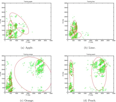
Figure 4: Fitted Gaussians after ten iterations of the Baum-Welch algorithm. We have six states with one Gaussian each. The two most dominant frequencies (features) are shown. Each green plus is represents a frame from a training speech signal. The stars are the means of each Gaussian, and the ellipses indicate their 75% confidence interval. Notice the higher frequencies present in the words containing unvoiced phonemes (‘peach’ and ‘orange’) compared to the words that do not (‘apple’ and ‘lime’).
were the number of hidden states, N, and the number of frequencies extracted from each frame, D. The cross-validation was therefore run with different values for these parameters, and the results are shown in table 1.
5
Discussion
N\D 2 3 4 5 6 7 8
2 21.9% 8.6%
3 21.0% 15.2% 9.5% 12.4% 1.9% 14.3% 5.7%
4 16.2% 11.4% 8.6% 5.7% 3.8% 6.7% 4.8%
5 13.3% 8.6% 9.5% 4.8% 2.9% 5.7% 4.8%
6 12.4% 10.5% 3.8% 5.7% 7.6% 6.7% 10.5%
7 15.2% 12.4% 6.7% 10.5% 7.6% 2.9% 8.6%
[image:8.595.142.456.99.211.2]8 12.4% 5.7%
Table 1: Misclassification rates for five-fold cross-validation with different values for the number of hidden states, N, and the number of frequencies extracted from each frame,D. Each five-fold cross-validation procedure takes about 7 minutes with the 105 utterances on a 2 GHz Intel Core 2 Duo (serial execution).
rates achieved. It should be noted that this system would not perform well if trained and tested with different speakers. This is because of the different frequency characteristics of different voices, especially for speakers of different gender.
We also experimented with increasing the number of training iterations for the Baum-Welch algorithm, including setting a threshold on the likelihood difference between steps. That, however, proved to have little benefit in practice; neither the execution time nor the misclassification rate showed any mentionable improvements over just fixing the number of iterations to 15. The reason why the execution time did not show any significant improvements is because most of the execution time is spent during feature extraction, and not in training.
It is also interesting to note that when N is too small, there are many ‘apple’s misclassified as ‘pineapple’s, and vice versa, due to the loss of temporal information.
Another important parameter is the number of samples in each frame. If the frame is too small, it becomes hard to pick out meaningful features, and if it is too large, temporal information is lost. However, due to time constraints, we did not test anything else than 80 samples for this project.
The concatenation of the training examples trains a probability of transitioning from the ‘last state’ to the ‘initial state’ that is not needed for classification. Rabiner gives a modified Baum-Welch algorithm for multiple training examples such that concatenation is not necessary, but that was not implemented during this project as the concatenation seemed to work well.
6
Conclusion and future work
recognizer.
The Matlab implementation along with the data set is published as open source and can be found athttp://code.google.com/p/hmm-speech-recognition/.
7
References
[1] L. R. Rabiner, “A tutorial on hidden Markov models and selected applications in speech recognition,” Proceedings of the IEEE, vol. 77, pp. 257–286, Feb 1989.
[2] C. M. Bishop,Pattern Recognition and Machine Learning (Information Science and
Statistics). Springer, 1st ed. 2006. corr. 2nd printing ed., October 2007.
[3] X. Huang, A. Acero, and H.-W. Hon, Spoken Language Processing: A Guide to