Comparative Analysis of Eigen face and Sparsity Based
Face Recognition Schemes
I
Dr. Renuka Devi S.M
,
IIE. Bhargavi
IDept. of Electronics and Communication Engineering, GNITS, Telangana, India.
IIPG Scholar, Dept. Of Electronics and Communication Engineering, GNITS, Telangana, India.
I. Introduction
With the advancement in the digital technology there is a strong need to safeguard the privacy of the user and the face recognition is one such application which helps us in preserving our assets. With its gaining popularity there has been a huge research in this area but primarily in Biometrics applications, Generally any face recognition system carries out three major tasks like face detection,
feature extraction and face recognition (or) face classification
[2]. In this paper we focus on face recognition section for static frontal face images, With a variant of face recognition methods implemented the top level categorization has divided them into three subcategories they are holistic matching methods which use the whole face region as the raw input to a recognition system like the Eigen face approach also known as Principle Component Analysis. The other two categories are Feature Based and Hybrid methods, where in local features like eyes, nose and mouth are
locally extracted and by using statistical methods the classification
is performed. The Hybrid methods make use of both local features
as well as the whole face region to perform classification [2]. Within each of these categories, further classification is possible.
Using principal-component analysis (PCA), many face recognition techniques have been developed, EigenFaces which use a
nearest-neighbour classifier; feature-line-based methods, which replace
the point-to-point distance with the distance between a point and the feature line linking two stored sample points. Fisher-faces which use Linear/Fisher discriminant analysis (FLD/LDA)
Bayesian methods, which use a probabilistic distance metric; and SVM methods, which use a support vector machine as the classifier
[2].
Many types of systems have been successfully applied to the task of face recognition, but they all have some advantages and disadvantages. Appropriate schemes should be chosen based on
the specific requirements of a given task. Most of the systems
here focus on the sub-task of recognition, but others also include automatic face detection and feature extraction, making them fully automatic systems [2].
In recent times there has been a huge research towards a topic known as Compressed Sensing also called as Compressed Sampling or Sparse sampling ,is a signal processing technique
for efficiently acquiring and reconstructing a signal, by finding
solutions to underdetermined linear systems. This is based on the principle that, through optimization, the sparsity of a signal can
be exploited to recover it from far fewer samples than required by the Shannon-Nyquist sampling theorem [12].
In this Paper a Comparative Study between Face Classification
methods like the Eigen-face dependent nearest neighbour approach also known as Principle Component Analysis as well as Sparse
Coding based Classification methods are considered.
II. Related Work
A. Eigen-Face Approach
Much of the previous work on automated face recognition has ignored the facts of just what aspects of the face stimulus are
important for identification, information content of face images
were studied using information theory concepts emphasizing local and global features. In the language of information theory we want to extract the relevant information in a face image, encode it as effectively as possible and compare face encoding with a database of models encoded similarly [1].
Eigen-face approach is a simple method for extracting the information contained in a collection of face images, independent of any judgement of features and uses this information to encode and compare individual face images [1].
Mathematically, we wish to find the principal components of
the distribution of faces or the eigenvectors of the covariance matrix of the set of face images, creating an image as a point (or vector) in a very high dimensional space, the eigen vectors are ordered each one accounting for a different amount of variation among face images these eigen vectors can be thought of as a set of features that together characterize the variation between face images [1].
The main idea for Eigen faces arises from the problem of performing recognition in a high dimensional space which can be addressed by mapping the image to a lower dimensional space and then by computing Eigen vectors.
Computation of the EigenFaces starts with obtaining face images I1, I2... IM(training faces).It is very important to note that the face
images must be centeredand of the same size [1]. Next is to
represent every image Iias a vector Γi .Then we need to compute
the average face vector Ψ by using the equation (1)
(1)
Then we compute the normalised images by subtracting the image
Abstract
Face Recognition has been one of the predominant research areas in the field of Biometric Analysis where there is a strong need for user friendly systems that can safeguard ones critical assets and privacy. Lately there were many algorithms that implemented face recognition systems but the theory of Compressed Sensing has gained popularity in recent times which enabled representation of data using Sparse Computations from Convex Optimization techniques. In this paper the comparative study between Nearest Neighbor Classifier method using Eigen faces and Sparse Classifier method is considered using a well-known face database which provides better Recognition rates even in various noise conditions.
Keywords
vectors from the average face vector Ψ, using the normalised faces
we then compute the covariance matrix using the equation (2)
(2)
= AAT
Where A= [Φ1, Φ 2 . . . ΦM] (N2xM matrix), we then compute the
eigenvectors ui of AAT. The matrix AAT is very large so it is not
practical to calculate it [5]. Then we consider the matrix AT A (M
x M matrix) and compute the eigenvectors vi of AT A using (3)
ATAv
i = μivi, (3)
The relationship between ui and vi is given by (4)
ui = Avi (4)
Thus, AAT and ATA have the same eigenvalues and their eigenvectors
are related as follows ui = Avi. Important points to note are that AAT
can have up to N2 eigenvalues and eigenvectors and ATA can have
up to M eigenvalues and eigenvectors and The M eigenvalues of
ATA (along with their corresponding eigenvectors) correspond to
the M largest eigenvalues of AAT (along with their corresponding
eigenvectors) [1].We need to compute the M best eigenvectors of AAT as u
i = Avi and it is important to normalize ui such that ||ui|| = 1.Then finally we keep only K eigenvectors (corresponding to the K largest eigenvalues), Representing faces onto this basis is done by subtracting each face with the mean Φi in the training set can
be represented as a linear combination of the best K eigenvectors
using (5)
(5)
Where wj = ujTΦ
i and here we call the u j’s EigenFaces. Each
normalized training face Φi is represented in this basis by a face
vector Ωi as (6)
(where i=1,2,M) (6)
Then face recognition of an test image is done by computing the
projection of that image by finding the Eigen face of the image
using wi=uiΦ then we compute the corresponding face vector,
finally the Euclidian distance between the face vectors of test
and training images is computed and least distance value is used to classify the image [1].
III. Methodology
A. Sparse Coding based Classifier method
In this method Face Recognition is performed using the Sparse Classifier in order to get optimized results with excellent accuracy. Sparse Representation helps us to study the Distinctive nature between the training samples to perform classification between
them.
According to the Theory of Compressive sensing the test samples are represented using the Over complete dictionary form by training samples used as base elements [12]. The test samples are represented as a linear combination of the training samples in order to study the sparse structure of test sample [4].
In this method we also study that, even in the presence of various noise conditions applied to test samples the theory of sparse coding
and classification helps us to achieve better results.
Initially a database of face images is considered, where part of database is used as training set and other as test set. With the training samples available, if a class of training set is considered then the test sample selected from the same class is represented as a linear combination of those training samples as equation (7) below [4]
y = αi,1 vi,1+ αi,2 vi,2 +…..+ αi,ni vi,ni (7)
where [vi,1, vi,2……. vi,ni]=Ai ϵ Rmxn and α
i,j ϵ R are some scalars,
j=1,2…ni. As the membership of the test sample is not known so
in a more general sense the above equation (7) is written as (8)
y = A x0 ϵ Rm (8)
Where A=[A1 A2… Ak]= [v1,1 v1,2 …….. vk,nk] is an Over-Complete
Dictionary and x0 isthe sparse vector whose coefficients are
associated with only a single class represented as non-zero elements [4].
The Sparse vector x0 is in linear form so it can be computed using
linearprogramming methods involving convex optimizations
according to the sparse coding theory. The sparsiest solution can
be obtained using a optimization method known as l0-minimization
but it is computationally non solvable in polynomial time and hence
is called as a NP-hard problem, alternatively l1-minimization is
employed to find the sparse vector, mathematically it is represented
as equation (9) below [8]
x1= subject to Ax = y (9)
The above equation is for noiseless condition, In noisy conditions the equation (10) is as follows
x1= subject to Ax - y ≤ ϵ (ϵ ≥ 0) 10)
The solution for l1 norm equation is found using linear programming
methods involving convex computations; l1 norm condition is
also called as Basis pursuit problem [8]. Basis Pursuit finds the
best representation of an image or a signal by minimizing the l1- norm of the components of x that is the coefficients in the
representation [7]. The components of x would be zero or as close to zero as possible. To better exploit the linear structure, we
classify y based on how good the coefficients are associated with
all training samples of each class in order to reproduce y. For a particular class i, we compute a characteristic function which
selects the coefficients associated with the ith class. The sparse
vector x and the Characteristic function being the new vector consists of only the nonzero entries of the sparse vector associated
with class i [4]. Using only the coefficients associated with the ith
class, we can approximate the given test sample y as = A δi(x1).
We then classify y based on these approximations by assigning it to the class that minimizes the residual between y and , The residual function is given as equation (11)
(11)
Using the Sparse Coding theory we can compute robust results in both noiseless and noisy conditions the identity and validity of a the test sample is also determined with high accuracy.
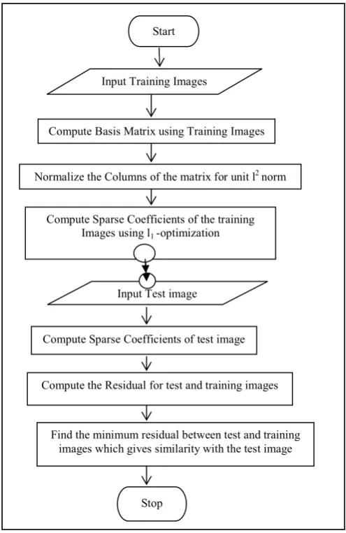
The Face recognition process using Sparse Coding in a sequence
Fig.1: Flow Chart Depicting the Process for Face Recognition
using Sparse Coding
IV. Experimental Results
The Performance of any Classification system is studied based
on the computations from Confusion matrix, which indicates the preciseness of the model in classifying the instances. A Confusion matrix is a table that is often used to describe the performance of a
classification model on a set of test data for which the true values
are known. Many objective metrics are derived from confusion matrix in order to predict the behavior of the model like the True Positives, True negatives, False Positives and False Negatives [11] .The confusion matrix for a binary class problem is as shown in Table (1)
The General Definitions for these metrics based on a ground truth about images from a database are defined as, If the instance is positive and it is classified as positive, it is counted as a true positive. If the instance is positive and if it is classified as negative,
it is counted as a false negative. If the instance is negative and
it is classified as negative, it is counted as a true negative. If the instance is negative and if it is classified as positive, it is counted
as a false positive [11].
The Important metrics computed using these metrics are
Sensitivity, Specificity and Accuracy given by equations
(12), (13) and (14)
Sensitivity = (12)
Specificity = (13)
Accuracy =
(14)
Table 1: Binary Class Representation of Confusion Matrix
Actual vs. Predicted Predicted Class 1 Predicted Class 2
Actual Class1 True Positive False Negative
Actual Class 2 False Positive True Negative
In this paper the concept of sparse representation of the images is studied by which we notice better recognition rates than the
traditional methods where Euclidian Distance based classifier is
used for classifying the instances.
The Face recognition by nearest neighbour using Eigen Face based
Classifier and Sparse coding based Classifier has been performed in Matlab using the ORL database comprising of 400 images with
40 classes where each class has10 images.[14]
The database has images with varying illumination and expressions
which also proves that these classifiers perform well in these conditions. Apart from these the classifier’s performance based on
sparse coding gives excellent results in case of noises like Gaussian and Salt & Pepper Noise with varying values. The accuracy of the
classifiers is also evaluated by treating the images to occlusion
also.
Table 2: Performance of the Classifier’s based on Noiseless
Condition Method
(Noiseless) True positive Rate False Positive Rate Accuracy
Sparse
Classifier 0.8650 0.0035 99.32 %
Eigen face
Classifier 0.0250 0.0240 95.12 %
Table 3: Performance of the Classifier’s based on Gaussian
Noise Method (Gaussian noise)
σ2=0.05,μ =0.09
True positive
Rate False positive Rate Accuracy
Sparse Classifier 0.7900 0.0054 98.94 %
Eigen face
Classifier 0.0245 0.0240 95.12 %
Table 4: Performance of the Classifier’s based on Salt & Pepper
Noise Method (Salt & Pepper noise)
Noise density (D)=0.05
True positive
Rate False positive Rate Accuracy
Sparse Classifier 0.8600 0.0036 99.30 %
Eigen face
Table 5: Performance of the Classifier’s based on Block Occlusion
Method
(Block Occlusion) (50 %)
True positive
Rate False positive Rate Accuracy
Sparse Classifier 0.5450 0.0117 97.72 %
Eigen face
Classifier 0.0230 0.0214 95.05 %
The Experimental Results in matlab using Eigen face approach with face images from ORL database [14] in noiseless and various
noisy conditions is as follows
Fig.2: Nearest neighbor based Classification using Eigen face in
noiseless condition
Fig.3: Nearest neighbor based Classification using Eigen face
for Gaussian noise with variance 0.01
Fig. 4: Nearest neighbor based Classification using Eigen face for
Salt & Pepper noise with noise density 0.01
Fig.5: Nearest neighbor based Classification using Eigen face in
case of Block Occlusion
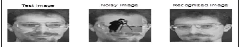
The Experimental Results using Sparse Classifier for various noisy
and noiseless conditions is as follows
Fig.6: Sparse Classification in Noiseless case
Fig.7: Sparse Classification in Gaussian Noise with Variance 0.01
Fig.8: Sparse Classification in Salt & Pepper Noise with noise
density 0.01
Fig.9: Sparse Classification in Block occlusion
V. Conclusion And Future Scope
In this paper the two Classification methods one based on Eigen face and other Sparse Classifier methods have been studied and implemented using Matlab for ORL database and it is observed
from the results that even in noiseless and various noisy conditions
the Performance of the Sparse Classifier is robust compared to one based on Eigen face Classifier and has high recognition rates
measured in terms of Accuracy computed from Confusion matrices.
This Sparse classifier can be used in biometric applications for finding the identity of users in various security conditions.
References
[1] M. Turk and A. Pentland, “EigenFaces for recognition,” in Proceedings of IEEE International Conference on Computer Vision and Pattern Recognition, 1991.
[2] W. Zhao, R. Chellappa, P. Phillips, and A. Rosenfeld, “Face recognition: A literature survey,” Acm Computing Surveys (CSUR), vol. 35, no. 4, pp. 399–458, 2003
[3] B. Olshausen and D. Field, “Sparse coding with an overcomplete basis set: A strategy employed by V1?” Vision Research, vol. 37, pp. 3311–3325, 1997.
[4] J. Wright, A. Yang, A. Ganesh, S. Sastry, and Y. Ma, “Robust face recognition via sparse representation,” IEEE Transactions on Pattern Analysis and Machine Intelligence, vol. 31, no. 2, pp. 210–227, 2009.
[5] P. Belhumeur, J. Hespanda, and D. Kriegman, “Eigenfaces vs. Fisherfaces: recognition using class specific linear projection,” IEEE Trans. On Pattern Analysis and Machine Intelligence, vol. 19, no. 7, pp. 711–720, 1997.
[6] A. Leonardis and H. Bischof, “Robust recognition using Eigen images,” Computer Vision and Image Understanding, vol. 78, no. 1, pp. 99–118, 2000.
[7] S. Chen, D. Donoho, and M. Saunders, “Atomic decomposition by basis pursuit,” SIAM Review, vol. 43, no. 1, pp. 129–159, 2001.
[8] E. Candes and J. Romberg, “L1-magic: Recovery of sparse signals via convex programming,”http://www.acm.caltech. edu/l1magic/, 2005.
[9] D. Donoho, “Neighbourly polytopes and sparse solution of underdetermined linear equations,” Dept. of Statistics TR 2005-4, Stanford University, 2005.
[10] D. Donoho and Y. Tsaig, “Fast solution of l1-norm minimization problems when the solution may be sparse,” preprint, http://www.stanford.edu/ tsaig/research.html, 2006.
[12] https://en.wikipedia.org/wiki/Sparse_approximation. [13] Matlab linprog, http://www.mathworks.se/hel p/optim/ug/
linprog.html