Precision-Recall versus Accuracy and the Role of Large Data Sets

(1)

The Thirty-Third AAAI Conference on Artificial Intelligence (AAAI-19)

Precision-Recall versus Accuracy and the Role of Large Data Sets

Brendan Juba, Hai S. Le

Washington University in St. Louis 1 Brookings Dr., St. Louis, MO 63130

bjuba@wustl.edu, hsle@wustl.edu

Abstract

Practitioners of data mining and machine learning have long observed that the imbalance of classes in a data set negatively impacts the quality of classifiers trained on that data. Numer-ous techniques for coping with such imbalances have been proposed, but nearly all lack any theoretical grounding. By contrast, the standard theoretical analysis of machine learn-ing admits no dependence on the imbalance of classes at all. The basic theorems of statistical learning establish the num-ber of examples needed to estimate the accuracy of a classi-fier as a function of its complexity (VC-dimension) and the confidence desired; the class imbalance does not enter these formulas anywhere. In this work, we consider the measures of classifier performance in terms of precision and recall, a measure that is widely suggested as more appropriate to the classification of imbalanced data. We observe that whenever the precision is moderately large, the worse of the precision and recall is within a small constant factor of the accuracy weighted by the class imbalance. A corollary of this obser-vation is that a larger number of examples is necessary and sufficient to address class imbalance, a finding we also illus-trate empirically.

1 Introduction

One of the primary concerns of statistical learning theory is to quantify the amount of data needed to reliably and ac-curately learn an unknown function that belongs to a given family, such as halfspaces, decision trees, neural networks, and so on. This quantity is often referred to as thesample complexityof learning the family of functions. The founda-tional results of statistical learning theory, first established by Vapnik and Chervonenkis (1971), assert that accurate learning of functions is possible using an amount of train-ing data that depends only on a parameter of the family of functions known as theVC-dimension. In particular, for dis-crete functions, this VC-dimension parameter is no larger than the number of bits needed to specify a member of the family in a given domain; often, it is proportional to this “description size” or the “number of parameters.” More-over, it is known that (up to the leading constant) the same number of examples is also necessaryto reliably identify a function that fits the data accurately (Blumer et al. 1989;

Ehrenfeucht et al. 1989; Anthony and Bartlett 1999; Han-neke 2016). Thus, the central message of statistical learn-ing theory is that this notion of model size controls the amount of data inherently needed for learning. In particu-lar, the same quantity suffices regardless of the distribution of the actual data, and thus regardless of the degree of class imbalance (“rarity” of positive examples) and so on.

In spite of the seemingly complete theoretical picture that these theorems paint, practitioners in data mining in par-ticular have been long concerned with the effects of class imbalance or rarity of classes in training data (Weiss 2004; He and Garcia 2009). These concerns led to much work on attempts to reduce the class imbalance by either dropping examples or synthesizing new ones. A crucial clue to the na-ture of the problem was provided by a substantial empirical study by Weiss and Provost (2003): In a study of a fixed de-cision tree learning algorithm on twenty-six data sets, they determined that indeed, the use of the natural class distri-bution provided close to the optimal accuracy (error rate) across almost all of the data sets, as standard learning the-ory suggests. But, on the other hand, they also found that for another metric– the area under the ROC curve (AUC) – the quality of the learned decision tree was significantly affected by the class imbalance of the data. Thus, their find-ings suggested that the sample complexity of some metrics of classifier quality, such as AUC, might depend on class imbalance, while others such as accuracy do not. And in-deed, Agarwal and Roth (2005) established that the sample complexity of learning under the AUC metric does depend on the class imbalance. More recently, Raeder et al. (2012) evaluated a variety of metrics and found empirically that ev-ery metric they consideredexceptfor accuracy had a depen-dence on the class imbalance. While the empirical studies leave open the question of whether these observations are artifacts of the particular algorithms used, we establish here that such a dependence is also inherent for theprecisionand recallof the learned classifier.

(2)

enters these expressions as an additional penalty over the usual expressions for accuracy.

A precise relationship between precision, recall, and ac-curacy (that holds with equality) was discovered previously by Alvarez (2002), and our bounds could also be derived easily from Alvarez’s equation. Interestingly, however, Al-varez did not interpret the consequences of his relation for the amount of data needed, which is our main contribution. Davis and Goadrich (2006) similarly showed that classi-fiers that dominate in the usual ROC space also dominate in precision-recall and vice-versa. Actually, results by Cortes and Mohri (2004) imply that precision-recall bounds are fundamentally different from AUC: for a fixed class imbal-ance and accuracy, various ranking functions may feature substantially different AUC scores, in contrast to precision-recall bounds. Hence, Davis and Goadrich’s result is incom-parable to ours.

Theoretical upper bounds on the sample complexity that is sufficient to achieve a given bound on the precision and recall were established previously by Liu et al. (2002) as part of a more general bound for partially supervised clas-sification and by Valiant (2006); similar upper bounds were established for the related “Neyman-Pearson classification task,” which is essentially an agnostic variant of learning with precision-recall bounds, by Cannon et al. (2002). Our contribution is that we show that the first set of bounds (for the realizable setting) cannot be substantially asymptotically improved and such a large amount of data is inherently nec-essary.1 To our knowledge, the only lower bound for any such task was obtained by Scott and Nowak (2005), who note that the false-negative and false-positive rates converge no faster than the overall error rate. Our quantitative conclu-sions are also similar to those obtained under the heursitic calculation used by Raeder et al. (2012) which simply calcu-lated the number of examples necessary to get, e.g., a train-ing set containtrain-ing100positive examples. This turns out to be a reasonable rule of thumb for, e.g., simple classifiers on data with10–100attributes, but we stress that it is not simply the number of positive examples that are relevant, as the vast number of negative examples is necessary to rule out the var-ious classifiers with an unacceptably high false alarm rate. In any case, we provide formal justification, showing that this number of examples isinherently necessaryfor success at the task in general, whereas the “100 positive examples” heuristic was largely grounded in intuition until now.

At a high level, our main observation is that achieving high precision and recall demands that our training data scales with the class imbalance; in particular, the methods for attempting to “correct” the imbalance by sub-sampling, or over-sampling, or generating new synthetic data dis-cussed above (all of which are topics of intense interest in certain areas) fundamentally should not provide any im-provement in precision-recall in general. By contrast, if we have sufficient training data (to achieve high accuracy), then

1

We observe that a small improvement over the bound obtain-able from Liu et al. follows immediately from Hanneke’s (2016) improved bound for accuracy, and we likewise strengthen Valiant’s upper bound from representation length to VC-dimension.

any standard learning method will do, without need for these special “imbalance-correcting” methods. We illustrate this finding empirically: We observe that for several standard off-the-shelf methods and several data sets featuring significant class imbalance, these imbalance-correcting methods do not provide reliable improvements in precision and recall, but adding more data always does significantly improve preci-sion and recall. We found that the only classifiers for which the imbalance correction methods frequently improve pre-cision and recall are depre-cision tree methods (here, Random Forest), where the techniques were originally developed.

But, we argue that in many applications, high precision is of the utmost importance, and in particular, in applications that suffer a severe class imbalance. We discuss two example domains here, one of hospital early-warning systems, and another in machine translation. The upshot is, unfortunately, these applications simply inherently require enormous data sets. This also partially explains a finding from the work on machine translation (Brants et al. 2007) that, from the usual standpoint of accuracy, is a bit puzzling: namely, as the size of the training data increased into the hundreds of billions of examples, Brants et al. found continued improvement in the quality of translations produced by a relatively simple method. The usual accuracy bounds suggest that the amount of training data necessary should only scale proportionally to the size of the model trained, and it is not clear why the rule for translation should need to be so large. But, we ob-serve that to even solve the problem of identifying which words to use in machine translation, we require high preci-sion (since most words are infrequently used), and hence our bounds establish that such an enormous number of examples is precisely what we should expect to require.

The rest of our paper is structured as follows: in Section 2, we discuss the importance of high-precision classifiers; in Section 3, we quantify the relationship between precision-recall and accuracy, derive sample complexity bounds for precision-recall, and discuss the need to use a large training data set; in Section 4, we present our experiments illustrating how using large training data improves the precision-recall on an imbalanced data set, while methods designed to sim-ply correct the class imbalance (e.g., from different data sets) generally do not achieve satisfactory precision and/or recall; in Section 5, we give our conclusions plus some advice for practitioners and finally, in Section 6, we sketch some pos-sible directions for future work.

2 The Importance of Precision

(3)

A first example concerns learning for alarm systems. Following a review by Amaral (2014), we find that early-warning systems for use in hospitals feature significant class imbalance and crucially rely on nontrivial precision, or else the alarms are ignored. We expect that this is broadly true of alarm systems in general.

A second example where the data is highly imbalanced (in a sense) and high precision is important can be found in machine translation. Here, we suppose that our training data consists of parallel texts in two languages, and we would like to train a system that, when given text in a source language, produces an equivalent text in the target language. Brants et al. (2007) designed a fairly successful system that, at its heart, simply counts the co-occurrence ofn-grams between the two texts and then performs some smoothing. The strik-ing findstrik-ing of Brants et al. was that a relatively simplistic scheme could achieve state-of-the-art performance merely so long as the amount of training data was enormous; in par-ticular, they found constant improvement when training their model on up to hundreds of billions of examples. It would not be so clear why so much data would be required if ac-curacy were the only issue, as there is no clear reason why many gigabytes of data should be necessary to specify the rules for translation.

The answer, of course, is that accuracy is not the key mea-sure in this case. Let us simply focus on the question of whether or not it is appropriate to use a given word in a sen-tence of the translated document, perhaps given a sensen-tence in the source language together with its context. In this case we have a simple binary classification task per word; but, we observe that most sentences contain infrequently used words.Intuitively, words that are informative and specific should be used in specific circumstances. We confirmed this intuition in practice by investigating the New York Times Annotated Corpus (Sandhaus 2008), a standard corpus con-taining more than 1.8 million articles. We first counted the frequency (with respect to sentences) of words in the cor-pus, that is, what fraction of sentences used that word. We take this fraction as an estimate of the imbalance of correct classifications for our function that predicts whether or not words should be used in the translation. Then, in order to translate a sentence, we must be able to correctly predict the words that should be used in the translated sentence. In par-ticular, it will follow from our bounds in Section 3 that it is the frequency of therarestword in the target sentence that determines the amount of data we require to reliably trans-late the sentence. As anticipated, for most sentences, this is quite high.

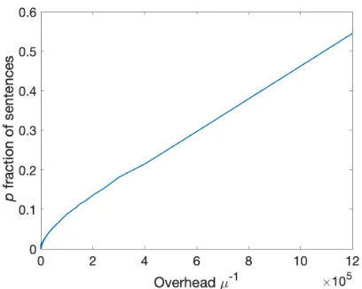
Concretely, we examine the fraction of sentences in which the rarest word appears in at least aµ-fraction of the sen-tences in the corpus; equivalently, as we will see in Sec-tion 3, this is the fracSec-tion of sentences for which an overhead of1/µin the sample complexity (over what would suffice for high-accuracy learning) suffices to achieve high preci-sion and recall. Since we were interested in the implications for translation, we used the Natural Language Toolkit (Bird, Klein, and Loper 2009) to filter out proper nouns for which (1) usage is likely abnormally infrequent and (2) various methods of directly rendering the word in a target language

by sound are frequently used for translation.2The results ap-pear in Figure 1: as a simple point of reference, observe that fewer than five in ten sentences have anadditional overhead of less than 1.2 million. This still gives no clear indication of how much data would be necessary to reach 95% of sen-tences, for example, except that it is surely well beyond 1.2 million examples, and likely beyond 12 billion (if we sup-pose≈104examples is necessary for learning such a model to high accuracy).

Figure 1: Proportion of sentences using only words occur-ring in a µ-fraction of sentences (and thus, learnable with overhead 1/µ) in the New York Times corpus (Sandhaus 2008). Fewer than 55% of sentences use only words that are sufficiently common to be learned with an overhead of any less than a factor of 1.2 million (see Section 3).

Now, we observe that unfortunately, at least moderately high precision and recall is important for this task. Indeed, given the high degree of imbalance, it is possible to achieve very high accuracy by simply predicting that these rare words are never used, or perhaps only used once in 50 mil-lion sentences—in other words, by sacrificing recall. This is of course undesirable, since then our machine translation system may not learn to use such informative words at all. It is also possible for the predictor to achieve high accuracy but low precision if it produces even a small number of false positives, that is nevertheless of the same order as the fre-quency with which the word should actually be used. In this case, the use of the word in the translation is uninforma-tive. That is, it may not provide any indication that the word should actually have appeared in the target text. This is also clearly undesirable, since it means that the use of a word is not connected to its context, i.e., it is “meaningless” (from an information-theoretic standpoint). As we will see next, as a consequence of our sample complexity lower bounds, if the training set does not contain billions of examples, then it is likely that either the recall is very low and hence the word is almost never used, or else the prediction that a word should

2

(4)

be used in the translated document may have low precision, and hence our word choice may be meaningless.

3 Precision-Recall Is Equivalent to

Imbalance-Weighted Accuracy

We now derive our main techincal bounds relating precision and recall to accuracy, and relate these to the sample com-plexity of classification tasks. We stress that while these are technically very simple, they have serious consequences for settings such as those discussed in Section 2.

Relating Accuracy, Imbalance, Precision, and

Recall

Suppose thatDis a distribution over examples with Boolean labels (x, b) ∈ X × {0,1} with a base positive rate of µ = PrD[b = 1]. For a hypothesish : X → {0,1}, the

accuracyofhisPr[h(x) =b]def= 1−acc; theprecisionof his PrD[b = 1|h(x) = 1]

def

= 1−prec, and therecall of hisPrD[h(x) = 1|b = 1]

def

= 1−rec. One often uses the expressions

tprdef= Pr

D[b= 1∧h(x) = 1] f pr

def = Pr

D[b= 0∧h(x) = 1]

tnrdef= Pr

D[b= 0∧h(x) = 0] f nr

def = Pr

D[b= 1∧h(x) = 0]

and it may be verified that our definitions above are equiva-lent to the perhaps more common expressions

1−prec= tpr

tpr+f pr 1−rec= tpr tpr+f nr 1−acc=tpr+tnr µ=tpr+f nr

Motivated by settings such as those discussed in Sec-tion 2, we will focus on the problem of learning classifiers with precision at least 50%. It turns out that in this case, pre-cision and recall are closely related to the (accuracy) error, scaled by the class imbalance:

Theorem 1 Suppose h : X → {0,1} has precision

greater than 1/2 inD. Thenmax def

= max{prec, rec} sat-isfiesµmax≤acc≤µ(rec+1−1precprec). In particular,

acc≤3µmax.

Proof: Note that rec = _tprf nr₊_{f nr} = f nr_µ , and since prec = _tprf pr₊_{f pr}, (1 −prec)f pr = prectpr and thus f pr≤µ₁₋1

precprecsincetpr≤µ. So, together,

acc=f pr+f nr≤µ(rec+ 1 1−prec

prec).

For the lower inequality, we already immediately have rec = f nr_µ ≤ acc_µ . Furthermore, since1−prec > 1/2, tpr+f pr < 2tpr, and hence tpr > f pr. We also find, since acc

µ =

f pr+f nr

tpr+f nr and forc ≥ 0andtpr > f pr ≥ 0

generally f pr_tpr₊+_cc ≥ f pr_tpr, acc

µ ≥

f pr tpr ≥

f pr

tpr+f pr = prec.

And so therefore, together, we obtainmax≤ acc_µ .

Sample Complexity Bounds For Precision-Recall

We now obtain the asymptotic sample complexity of si-multaneously achieving high precision and high recall as a corollary of Theorem 1 and the known bounds for accuracy. Again, theVC-dimension, introduced by Vapnik and Cher-vonenkis (1971), is the parameter controlling these bounds:

Definition 2 (VC-dimension) We say that a set of points in a domainX is shatteredby a set of Boolean classifiersC

on the domainX if every possible labeling of the set is ob-tained by some classifier inC. We then say thatC has VC-dimensiond∈Nif some set ofdpoints inXis shattered by C, and no set ofd+ 1points is shattered. If for everyd∈N

every set ofdpoints is shattered byC, then we say thatChas infinite VC-dimension (“d=∞”).

The asymptotic sample complexity of obtaining a given accuracy is now known exactly:

Theorem 3 (Hanneke 2016) For a family of classifiers of VC-dimensiond, with probability1−δ, every classifier that is consistent withO 1(d+ log1_δ)examples drawn from a distributionDon labeled examples, has error rate at most (accuracy1−) onD.

A matching lower bound was proved in two parts; first, a Ω(1log1_δ) lower bound was obtained by Blumer et al. (1989), and subsequently an Ω(d/)bound was proved by Ehrenfeucht et al. (1989). Together, these yield a matching lower bound:

Theorem 4 (Blumer et al. and Ehrenfeucht et al.) For a family of classifiers of VC-dimensiond, there is a constant δ0such that forδ ≤δ0, unlessΩ 1(d+ log1_δ)examples are drawn from a distributionDon labeled examples, with probability at leastδsome classifier in the family with ac-curacy less than 1 − on D is consistent with all of the examples.

Since any classifier with precision greater than 1/2and accuracy 1 −acc must have precision and recall at least 1 − acc

µ , we find that to obtain precision and recall 1− max, it suffices to simply learn to accuracy1−µacc, i.e.,

O_µ1

max(d+ log

1

δ)

examples suffice.3

Corollary 5 (Upper bound for precision-recall) For any family of Boolean classifiers C of VC-dimension d on a domain X and any distributionD on X, suppose we are given examples drawn fromD labeled byc ∈ C such that Pr[c(x) = 1] = µ. Then with probability1−δany

clas-sifierc0 ∈ C that is consistent withO 1

µmax(d+ log

1

δ)

examples achieves precision and recall1−max.

And conversely, since (unless the precision is less than 1/2) either the precision or recall is at most 1− acc

3µ, we

find that unlessΩ 1

µmax(d+ log

1

δ)

examples are drawn from D, if δ < δ0, then with probability at leastδ, some hypothesis that is consistent with all of the examples has

3

Note that although Theorem 1 would not apply tomax>1/2,

(5)

accuracy less than1−3µmax; hence some such hypothesis has either precision or recall that is less than1−max:

Corollary 6 (Lower bound for precision-recall) For a family of classifiers of VC-dimension d, there is a con-stant δ0 such that for δ ≤ δ0 and max < 1/2, unless

Ω_µ1

max(d+ log

1

δ)

examples are drawn from a

distri-bution D on labeled examples, with probability at least δ some classifier in the family with precision or recall less than1−maxonDis consistent with all of the examples.

Recap As we noted in the introduction, similar upper bounds have been proved for a variety of cases by many au-thors, and here we can exploit the recent work by Hanneke to unify and/or improve all such bounds for the “realizable” case. A perhaps more important novelty here is the (match-ing) lower bound, which had not been studied previously. As we will discuss shortly, the presence of the1/µpenalty in these bounds is quite significant: it means that

1. in contrast to learning under the accuracy objective, when we seek precision greater than 50%, class imbalance does impose a cost on learning, and

2. the problem of coping with imbalanced data is entirely one of learning to unusually high accuracy, and hence one of collecting a large enough data set since training set size is what controls generalization error.4

We note that these bounds also imply that the algorithms for learning to abducek-DNFs of Juba (2016) have optimal sample complexity, when we consider the maximum “plau-sibility” (equal to the true positive rate) for distributions ac-tually labeled by a k-DNF. The same sample complexity lower bound also applies to the related problem of condi-tional linear regression under the sup norm (Juba 2017).

We can similarly obtain bounds for the sample complexity of achieving a given boundmaxon the precision and recall inagnostic(a.k.a.non-realizable) learning, using the known bounds in that setting. Specifically, we obtain the following bounds for approximate agnostic learning

Corollary 7 (c.f. Anthony and Bartlett 1999) There is a constant δ0 > 0 such that the following holds. For any family of Boolean classifiersCof VC-dimensiondon a do-mainX and any distribution D overX ×{0,1}, suppose we are given examples drawn from D such that Pr[b = 1] = µand minc∗_∈CPr[c∗(x) 6= b] = ∗_acc. Put∗_prec =

Pr[b 6= 1|c∗(x) = 1],_rec∗ = Pr[c∗(x) 6= 1|b = 1], and ∗_max = max{∗_prec, ∗_rec}. Then for δ < δ0, α > 1, and 3α∗max <1/2,Θ

1

µ∗

max(α−1)2(d+ log

1

δ)

examples are

necessary to return a classifier that with probability1−δ satisfiesmax≤(α/3)∗maxand sufficient to return a classi-fier that with probability1−δsatisfiesmax≤3α∗max. Proof: We first observe that indeed,∗

acc ≤ 3µ∗max and µ∗_max ≤∗_accsince the correspondingc∗ ∈ C attaining the

4

In particular, this conclusion follows when the generalization error is the primary component of test error. This is true by defini-tion in the “realizable” setting where zero training error is always achievable, and is often true in practice more generally.

minimum on the RHS can be used to bound the LHS in each case. Therefore, sinceO 1

∗

acc(α−1)2

(d+ log1

δ)

examples suffice to learn a classifier withacc ≤ α∗acc, we find that since ∗

acc ≤ 3µ∗max andµmax ≤ acc, that for such a classifiermax≤3α∗max.

Similarly, if we do not useΩ∗ 1

acc(α−1)2(d+ log

1

δ)

ex-amples there is a distributionD such that with probability at leastδwe return a classifier withacc > α∗acc. For this distribution, since∗_acc ≥µ∗_max, with probability at leastδ we are returning a classifier withacc > µα∗max. Now, for this classifier,max≥₃acc_µ , so it hasmax> α∗max/3.

Since the known time-efficient algorithms for agnostic learning (Awasthi, Blum, and Sheffet 2010, e.g.) obtain an approximation factor α that grows polynomially with the dimension (so in particular α = ω(1)), these bounds are adequate to understand how many examples are asymptoti-cally necessary for such guarantees; indeed, Daniely (2016) shows evidence that polynomial-time algorithms for agnos-tic learning of halfspaces (or any stronger class) must suffer an approximation factor of α = ω(1), so it seems likely that these bounds address all such algorithms. In particu-lar, we observe that they again pay the same1/µpenalty as in realizable learning. Nevertheless, it would still be nice to understand the sample complexity of precision and recall for agnostic learning more precisely. In particular, we do not ob-tain any bounds for the additive-error agnostic learning task. We leave this for future work.

4 Experiment

To verify our theoretical conclusion that using more train-ing data is necessary to cope with class-imbalance, we per-formed an experiment on a severely imbalanced data set, comparing the performance (i.e. precision and recall) be-tween various techniques that are used for dealing with im-balanced data and training on a larger data set without using these techniques. Such techniques include: Random under-sampling, which randomly removes samples from the major-ity class; Random oversampling, which randomly expands the minority class (He and Garcia 2009); Easy Ensemble (Liu, Wu, and Zhou 2006), which uses random subsets of the majority class to improve balance and form multiple classifiers; NearMiss (Zhang and Mani 2003), which applies K-Nearest Neighbor (K-NN) to choose a number of ma-jority examples around each minority example. In addition, we also applied the Synthetic minority oversampling tech-nique (SMOTE) (Chawla et al. 2002), which makes up data based on the feature space similarities among minority ex-amples, with the integration with condensed nearest neigh-bor (CNN), edited nearest neighneigh-bor (ENN), Tomek links (Batista, Prati, and Monard 2004), and support vector ma-chines (SVM) (Akbani, Kwek, and Japkowicz 2004).

(6)

mi-Table 1: Data set characteristics

Dataset Size Attributes Target Maj/Min abalone 4,177 8 Ring = 7 9.7:1

letter 20,000 16 A 24.3:1

satimage 6,435 36 class 4 9.3:1 drug discovery 1,062,230 152 class 1 16.1:1

nority class) less than 5. In addition, we also added a large data set (about 1 million examples) that was used for a vir-tual screening task in drug discovery (Garnett et al. 2015). Key characteristics of these data sets are summarized in Ta-ble 1. For the scope of this experiment, for all data sets, we merged all majority classes into a single majority class.

Experiment Setup For this experiment, we used the Python scikit-learn library (Pedregosa et al. 2011) with the imbalanced-learn package (Lemaˆıtre, Nogueira, and Aridas 2016) that contains a number of re-sampling techniques that are commonly used for classifying imbalanced data. In the first experiment, all data sets were stratified into ten folds. We selected data in one fold as small training set, eight folds aslargetraining set, and the last fold astest set. For thesmalltraining set, we created different learning models by re-sampling data in that fold using various techniques mentioned earlier (along with an unmodified version) be-fore training them using one of several standard classifiers. Meanwhile, for thelargetraining set, we simply trained the model using the same classifier. All models are then tested on the remaining fold. For each model, we recorded the pre-cision and recall values. We used K-Nearest Neighbor, Lo-gistic Regression, SVM, and Random Forest as our choices of standard classifiers. For the preprocessing algorithms, we used the following settings of our hyperparameters: we set the“sampling strategy”to“float”, and left other hyperpa-rameters default for the imbalanced-learn package imple-mentation. For K-Nearest Neighbor, we performed valida-tion to determine k. k was set to 5 for most of the data sets, except forletter(k= 3). For the other classifiers, we set“class weight”to“balanced” and left all other hyper-parameters as default.

We note that K-Nearest Neighbor is not a classifier of bounded VC-dimension, so the analysis of the previous sec-tion does not actually apply. Analyses of K-Nearest Neigh-bor (Gyorfi, Lugosi, and Devroye 1996, e.g.) depend on smoothness properties of the data that would seem to be fa-vorable for the intuitions behind techniques like SMOTE. Nevertheless, we will see that even in cases where K-Nearest Neighbor is rather successful, these techniques for directly correcting class imbalance not only do not strictly help, they may actually harm precision and recall.

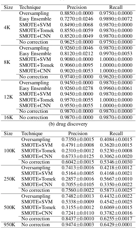
In addition, to verify the the relationship between the number of examples and the performance in imbalanced and balanced settings, we ran a fine-grained experiment with in-creasing sizes of the data fold. We chose two large data sets (letteranddrug discovery); selected the methods that seemed to be working on them from the first experiment;

then repeated the first experiment with K-Nearest Neighbor, varying the size of the smalltraining set. For both experi-ments, to get stable results, we repeated the experiment 100 times and recorded the mean and standard deviation values.

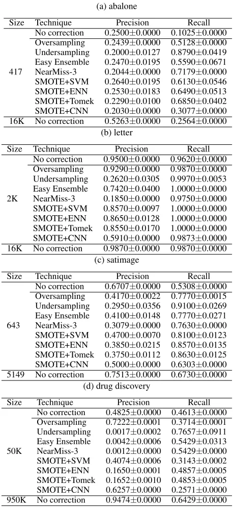
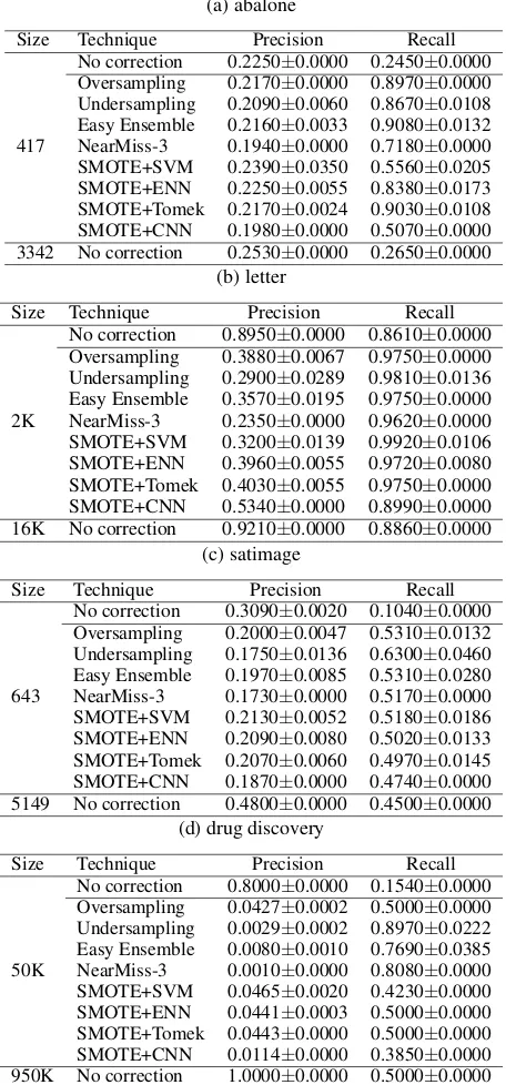
Results and Discussion For the first experiment, results are shown in Table 2 (K-NN), Table 3 (Logistic Regression), Table 4 (SVM), and Table 5 (Random Forest), which con-tains the precision and recall results of training on the results of sampling techniques on the small training set as well as the results of training on two uncorrected data sets, one small and one large. For almost all of the data sets, the results sug-gest that we can improve the precision and recall simply by increasing the size of the training set, and this effect is not matched by applying the methods for class imbalance. In-deed, the only exception(s) to this were SMOTE+SVM and SMOTE+ENN with Random Forest on the drug discovery data set; we will discuss this in more detail later. Meanwhile, compared to simply performing no correction, the methods aimed at correcting the imbalance frequently improve re-call at the cost of precision or vice versa. They might even harm either precision, recall, or both. Except when Ran-dom Forest was used, the only seven exceptions (out of 96 conditions) where both precision and recall improved were SMOTE+SVM and SMOTE+ENN forabalonewith K-NN and logistic regression and Oversampling, SMOTE+SVM, and SMOTE+ENN forletterwith SVM.

In the case of Random Forest, SMOTE+SVM and SMOTE+ENN improved both precision and recall on all data sets except satimage. Easy Ensemble improved both precision and recall on abalone. Oversampling improved both precision and recall for both abalone andletter, and SMOTE+Tomek also improved both forletter. We note that no method improved both precision and recall for satim-age using Random Forest. We believe that the reason for these methods’ marked success on Random Forest is as sug-gested by Japkowicz and Stephen (2002): the imbalance cor-rection methods were designed using a decision tree clas-sifier as their benchmark, and hence narrowly address the issues decision tree classifiers face. Nevertheless, as noted by Japkowicz and Stephen in the case of accuracy, these methods do not generalize well across different classifiers (e.g. SVM). What is different for precision-recall is that our theoretical bounds show that class imbalance still poses an inherent problem for all classifiers. In particular, a method like SVM will show the effect of class imbalance under precision-recall but not accuracy. (Indeed, Japkowicz and Stephen observed that the accuracy achieved by SVM was unaffected by the class imbalance.) We stress that the per-formance of an algorithm on a given data distribution is not simply determined by the class imbalance: it also depends on how well the representations used can fit the data distri-bution, and how successful the algorithm is at fitting them.

(7)

as the size of the training set increased, but still imbalance correction methods showed no clear benefit. It suggests that precision and recall indeed scale by the size of the train-ing set, strengthentrain-ing our observation that the the effect of adding more data dominates the impact of imbalance correc-tion methods in terms of precision and recall performance.

In general, both experiments corroborate our theoretical conclusion that training on a large data set would improve the performance (i.e. precision and recall) of the class im-balance problem, and that the methods aimed at simply “cor-recting” the class imbalance are not reliable. Thus, our ad-vice in general is not to rely on the imbalance correction methods as a means of achieving high precision and recall whereas acquiring more data, when available, does help.

5 Ramifications and Advice to Practitioners

Our main finding is negative: in the presence of severe class imbalance, it is not possible to reliably achieve high pre-cision and recall unless one possesses a large amount of training data. In some typical applications, such as machine translation, we observed that the amount of training data needed to obtain a meaningful indication of what word to use in a translation by statistical methods alone borders on the implausible. We find that methods that have been pro-posed to correct the class imbalance directly simply should not work, since there is an inherent statistical barrier. (And conversely, if there were enough data available, then stan-dard machine learning techniques will do and the methods to correct the imbalance are not needed.)

To a practitioner faced with such a task, simply giving up is not an option. Our results suggest inherent limita-tions of purely data-driven methods for such tasks: one sim-ply should not trust machine learning algorithms to provide rules of high precision and recall on a typical size data set with high imbalance any more than one would trust them to provide high accuracy rules on a data set of a handful of examples (e.g., a training set of size 10-50 in practice). The advice we would give to such a practitioner would be the same in both cases, that is, to try to exploit some kind of prior knowledge about the domain.

For example, in the case of natural language tasks, there may not be enough data to learn the appropriate usage of un-common, informative words. But,definitionsof these words that approximately indicate their usage are readily available in dictionaries. Indeed, we observe that humans learning a language (whether it is their native language or a foreign language) do not learn many of these words from everyday speech, but rather through definitions that are explicitly pro-vided in language classes or dictionaries. Thus, while statis-tical methods might be very good at learning the usage of common words or phrases, we believe that the knowledge provided by the rules in a dictionary should be used to com-plement this understanding of the basic language to achieve adequate precision for tasks such as machine translation.

Similarly, in the case of the hospital early warning sys-tems, much is known about conditions such as cardiac arrest. We hope that this explicit knowledge, properly encoded and integrated into the learning algorithm, could be used to help achieve high precision in the classification task in spite of

Table 2: Precision and Recall values for models that apply different imbalance-correction methods on thesmall train-ing set versus K-NN alone ustrain-ing thelargetraining set

(a) abalone

Size Technique Precision Recall

417

No correction 0.2500±0.0000 0.1025±0.0000 Oversampling 0.2439±0.0000 0.5128±0.0000 Undersampling 0.2000±0.0127 0.8790±0.0419 Easy Ensemble 0.2470±0.0195 0.5590±0.0671 NearMiss-3 0.2044±0.0000 0.7179±0.0000 SMOTE+SVM 0.2640±0.0195 0.6130±0.0546 SMOTE+ENN 0.2530±0.0183 0.6490±0.0513 SMOTE+Tomek 0.2290±0.0100 0.6850±0.0402 SMOTE+CNN 0.2030±0.0000 0.3077±0.0000 16K No correction 0.5263±0.0000 0.2564±0.0000

(b) letter

2K

(c) satimage

643

No correction 0.6707±0.0000 0.5308±0.0000 Oversampling 0.4170±0.0022 0.7770±0.0015 Undersampling 0.2950±0.0356 0.9100±0.0269 Easy Ensemble 0.4100±0.0148 0.7770±0.0271 NearMiss-3 0.3079±0.0000 0.7630±0.0000 SMOTE+SVM 0.4700±0.0070 0.8100±0.0123 SMOTE+ENN 0.3850±0.0215 0.8570±0.0135 SMOTE+Tomek 0.3750±0.0112 0.8630±0.0125 SMOTE+CNN 0.5000±0.0000 0.6303±0.0000 5149 No correction 0.7513±0.0000 0.6730±0.0000

(d) drug discovery

50K

the relatively small amount of data available to train such systems.

(8)

Table 3: Precision and Recall values for models that apply different imbalance-correction methods on thesmall train-ing set versus Logistic Regression alone ustrain-ing the large training set

(a) abalone

417

(b) letter

2K

(c) satimage

643

(d) drug discovery

50K

will do for such tasks. Some kind of richer representation of knowledge and classification decisions will be necessary to achieve high precision.

6 Future Work

As mentioned earlier, we did not obtain any bounds for the sample complexity of additive-error agnostic learning. This

Table 4: Precision and Recall values for models that apply different imbalance-correction methods on thesmall train-ing set versus SVM alone ustrain-ing thelargetraining set

(a) abalone

417

(b) letter

2K

(c) satimage

643

(d) drug discovery

50K

(9)

Table 5: Precision and Recall values for models that apply different imbalance-correction methods on thesmall train-ing set versus Random Forest alone ustrain-ing thelargetraining set

(a) abalone

417

(b) letter

2K

(c) satimage

643

(d) drug discovery

50K

the most desirable metric (e.g. when the number of true neg-ative examples is large). We might also consider examining the sample complexity of learning under other metrics such as the Brier Score, H-measure, F-measure, etc. The empir-ical results of Raeder et al. (2012) suggest that these mea-sures likewise will depend on the class imbalance, but the question is (of course) how precisely achieving bounds on

Table 6: Precision and Recall values for models that apply different sampling methods versus K-NN alone on varying sizes of data sets

(a) letter

4K

Oversampling 0.8850±0.0000 0.9750±0.0000 Easy Ensemble 0.7270±0.0246 0.9890±0.0072 SMOTE+SVM 0.8490±0.0068 0.9870±0.0000 SMOTE+Tomek 0.8550±0.0059 0.9870±0.0000 SMOTE+CNN 0.8520±0.0049 0.9870±0.0000 No correction 0.9625±0.0000 0.9750±0.0000

8K

Oversampling 0.9260±0.0046 0.9870±0.0000 Easy Ensemble 0.8120±0.0212 0.9970±0.0053 SMOTE+SVM 0.9080±0.0000 1.0000±0.0000 SMOTE+Tomek 0.9060±0.0095 1.0000±0.0000 SMOTE+CNN 0.9020±0.0053 1.0000±0.0000 No correction 0.9740±0.0000 0.9620±0.0000

12K

Oversampling 0.9450±0.0000 0.9870±0.0000 Easy Ensemble 0.9260±0.0278 0.9960±0.0061 SMOTE+SVM 0.9450±0.0000 0.9870±0.0000 SMOTE+Tomek 0.9570±0.0055 1.0000±0.0000 SMOTE+CNN 0.9550±0.0055 1.0000±0.0000 No correction 0.9870±0.0000 0.9870±0.0000 16K No correction 0.9870±0.0000 0.9870±0.0000

(b) drug discovery

100K

Oversampling 0.7350±0.0015 0.4084±0.0015 SMOTE+SVM 0.4791±0.0008 0.3620±0.0015 SMOTE+Tomek 0.2310±0.0012 0.5230±0.0008 SMOTE+CNN 0.6733±0.0125 0.3062±0.0020 No correction 0.6042±0.0015 0.5346±0.0030

250K

Oversampling 0.7413±0.0016 0.4218±0.0012 SMOTE+SVM 0.5164±0.0005 0.4168±0.0021 SMOTE+Tomek 0.2857±0.0016 0.5667±0.0010 SMOTE+CNN 0.7055±0.0105 0.3350±0.0022 No correction 0.7560±0.0022 0.5873±0.0025

500K

Oversampling 0.7482±0.0013 0.4432±0.0022 SMOTE+SVM 0.5338±0.0009 0.4542±0.0025 SMOTE+Tomek 0.3155±0.0012 0.6069±0.0015 SMOTE+CNN 0.7241±0.0110 0.3782±0.0016 No correction 0.8437±0.0010 0.6255±0.0017 950K No correction 0.9474±0.0003 0.6429±0.0001

these alternative measures of loss depends on these parame-ters. Relatedly, the top-k metrics are often used in informa-tion retrieval to overcome the problem of low precision in such challenging settings. It would be interesting to better understand the sample complexity of these metrics as well.

Acknowledgements

This work was supported by an AFOSR Young Investigator award and NSF award CCF-1718380. We thank R. Garnett, S. Das, and our anonymous reviewers for their suggestions.

References

Agarwal, S., and Roth, D. 2005. Learnability of bipartite ranking functions. InInternational Conference on Computational Learning Theory, 16–31. Springer.

(10)

Sup-port Vector Machines to Imbalanced Datasets. Berlin, Heidelberg: Springer Berlin Heidelberg. 39–50.

Alvarez, S. A. 2002. An exact analytical relation among re-call, precision, and classification accuracy in information retrieval. Technical Report BC-CS-2002-01, Computer Science Department, Boston College.

Amaral, A. C. K. B. 2014. The art of making predictions: Statistics versus bedside evaluation. American J. Respiratory and Critical Care Medicine190(6):598–599.

Anthony, M., and Bartlett, P. 1999. Neural Network Learning: Theoretical Foundations. Cambridge: Cambridge University Press. Awasthi, P.; Blum, A.; and Sheffet, O. 2010. Improved guarantees for agnostic learning of disjunctions. InProc. 23rd COLT, 359– 367.

Batista, G. E. A. P. A.; Prati, R. C.; and Monard, M. C. 2004. A study of the behavior of several methods for balancing machine learning training data.SIGKDD Explor. Newsl.6(1):20–29. Bird, S.; Klein, E.; and Loper, E. 2009. Natural Language Pro-cessing with Python. O’Reilly Media, Inc., 1st edition.

Blumer, A.; Ehrenfeucht, A.; Haussler, D.; and Warmuth, M. K. 1989. Learnability and the Vapnik-Chervonenkis dimension. J. ACM36(4):929–965.

Brants, T.; Popat, A. C.; Xu, P.; Och, F. J.; and Dean, J. 2007. Large language models in machine translation. InProceedings of the 2007 Joint Conference on Empirical Methods in Natural Lan-guage Processing and Computational Natural LanLan-guage Learning (EMNLP-CoNLL), 858–867. Prague, Czech Republic: Association for Computational Linguistics.

Cannon, A.; Howse, J.; Hush, D.; and Scovel, C. 2002. Learning with the Neyman-Pearson and min-max criteria. Technical Report LA-UR-02-2951, Los Alamos National Laboratory.

Chawla, N. V.; Bowyer, K. W.; Hall, L. O.; and Kegelmeyer, W. P. 2002. SMOTE: synthetic minority over-sampling technique.JAIR 16:321–357.

Cortes, C., and Mohri, M. 2004. AUC optimization vs. error rate minimization. InAdvances in neural information processing sys-tems, 313–320.

Daniely, A., and Shalev-Shwartz, S. 2016. Complexity theoretic limtations on learning DNF’s. InProc. 29th COLT, volume 49 of JMLR Workshops and Conference Proceedings. 1–16.

Davis, J., and Goadrich, M. 2006. The relationship between precision-recall and ROC curves. InProc. 23rd ICML, 233–240. Ehrenfeucht, A.; Haussler, D.; Kearns, M.; and Valiant, L. 1989. A general lower bound on the number of examples needed for learn-ing.Inf. Comp.82:247–261.

Garnett, R.; G¨artner, T.; Vogt, M.; and Bajorath, J. 2015. Intro-ducing the ‘active search’ method for iterative virtual screening. Journal of Computer-Aided Molecular Design29(4):305–314. Gyorfi, L. D. L.; Lugosi, G.; and Devroye, L. 1996.A probabilistic theory of pattern recognition. New York: Springer.

Hanneke, S. 2016. The optimal sample complexity of PAC learn-ing.JMLR17(38):1–15.

He, H., and Garcia, E. A. 2009. Learning from imbalanced data. IEEE Trans. Knowledge and Data Eng.21(9):1263–1284. Japkowicz, N., and Stephen, S. 2002. The class imbalance prob-lem: A systematic study.Intelligent data analysis6(5):429–449. Juba, B. 2016. Learning abductive reasoning using random exam-ples. InProc. 30th AAAI, 999–1007.

Juba, B. 2017. Conditional sparse linear regression. InProc. 8th ITCS, volume 67 ofLIPIcs.

Lemaˆıtre, G.; Nogueira, F.; and Aridas, C. K. 2016. Imbalanced-learn: A python toolbox to tackle the curse of imbalanced datasets in machine learning.CoRRabs/1609.06570.

Liu, B.; Lee, W. S.; Yu, P. S.; and Li, X. 2002. Partially supervised classification of text documents. InProc. 19th ICML, 387–394. Liu, X.; Wu, J.; and Zhou, Z. 2006. Exploratory under-sampling for class-imbalance learning. InSixth International Conference on Data Mining (ICDM’06), 965–969.

Pedregosa, F.; Varoquaux, G.; Gramfort, A.; Michel, V.; Thirion, B.; Grisel, O.; Blondel, M.; Prettenhofer, P.; Weiss, R.; Dubourg, V.; Vanderplas, J.; Passos, A.; Cournapeau, D.; Brucher, M.; Perrot, M.; and Duchesnay, E. 2011. Scikit-learn: Machine learning in Python. Journal of Machine Learning Research12:2825–2830. Raeder, T.; Forman, G.; and Chawla, N. V. 2012. Learning from imbalanced data: Evaluation matters. InData Mining: Foundations and Intelligent Paradigms, volume 23 ofIntelligent Systems Refer-ence Library. Berlin: Springer. 315–331.

Sandhaus, E. 2008. The New York Times annotated corpus ldc2008t19. DVD.

Scott, C., and Nowak, R. 2005. A Neyman-Pearson approach to statistical learning.IEEE Trans. Inf. Theory51(11):3806–3819. Valiant, L. G. 2006. Knowledge infusion. InProc. AAAI-06, 1546– 1551.

Vapnik, V., and Chervonenkis, A. 1971. On the uniform conver-gence of relative frequencies of events to their probabilities.Theory of Probability and its Applications16(2):264–280.

Weiss, G. M., and Provost, F. 2003. Learning when training data are costly: The effect of class distribution on tree induction. JAIR 19:315–354.

Weiss, G. M. 2004. Mining with rarity: A unifying framework. ACM SIGKDD Explorations Newsletter6(1):7–19.