Redundancy Techniques for Straggler Mitigation in
Distributed Optimization and Learning
Can Karakus [email protected]
Amazon Web Services∗
East Palo Alto, CA 94303, USA
Yifan Sun [email protected]
Department of Computer Science University of British Columbia Vancouver, BC, Canada
Suhas Diggavi [email protected]
Department of Electrical and Computer Engineering University of California, Los Angeles
Los Angeles, CA 90095, USA
Wotao Yin [email protected]
Department of Mathematics
University of California, Los Angeles Los Angeles, CA 90095, USA
Editor:Tong Zhang
Abstract
Performance of distributed optimization and learning systems is bottlenecked by “straggler” nodes and slow communication links, which significantly delay computation. We propose a distributed optimization framework where the dataset is “encoded” to have an over-complete representation with built-in redundancy, and the straggling nodes in the system are dynamically treated as missing, or as “erasures” at every iteration, whose loss is com-pensated by the embedded redundancy. For quadratic loss functions, we show that under a simple encoding scheme, many optimization algorithms (gradient descent, L-BFGS, and proximal gradient) operating under data parallelism converge to an approximate solution even when stragglers are ignored. Furthermore, we show a similar result for a wider class of convex loss functions when operating under model parallelism. The applicable classes of objectives covers several popular learning problems such as linear regression, LASSO, support vector machine, collaborative filtering, and generalized linear models including lo-gistic regression. These convergence results are deterministic, i.e., they establish sample path convergence for arbitrary sequences of delay patterns or distributions on the nodes, and are independent of the tail behavior of the delay distribution. We demonstrate that equiangular tight frames have desirable properties as encoding matrices, and propose effi-cient mechanisms for encoding large-scale data. We implement the proposed technique on Amazon EC2 clusters, and demonstrate its performance over several learning problems, in-cluding matrix factorization, LASSO, ridge regression and logistic regression, and compare the proposed method with uncoded, asynchronous, and data replication strategies.
∗. Work done while at University of California, Los Angeles.
c
Keywords: Distributed optimization, straggler mitigation, proximal gradient, coordinate descent, restricted isometry property
1. Introduction
Solving learning and optimization problems at present scale often requires parallel and distributed implementations to deal with otherwise infeasible computational and memory requirements. However, such distributed implementations often suffer from system-level issues such as slow communication and unbalanced computational nodes. The runtime of many distributed implementations are therefore throttled by that of a few slow nodes, called stragglers, or a few slow communication links, whose delays significantly encumber the overall learning task Dean and Barroso (2013). In this paper, we propose a distributed optimization framework based on proceeding with each iteration without waiting for the stragglers, and encoding the dataset across nodes to add redundancy in the system in order to mitigate the resulting potential performance degradation due to lost updates.
We consider the master-worker architecture, where the dataset is distributed across a set of worker nodes which directly communicate to a master node to optimize a global objective. The encoding framework consists of an efficient linear transformation (coding) of the dataset that results in an overcomplete representation, which is then partitioned and distributed across the worker nodes. The distributed optimization algorithm is then performed directly on the encoded data, with all worker nodes oblivious to the encoding scheme, i.e., no explicit decoding of the data is performed, and nodes simply solve the effective optimization problem on the encoded data. In order to mitigate the effect of stragglers, in each iteration, the master node only waits for the first k updates to arrive from the m worker nodes (where k ≤ m is a design parameter) before moving on; the remainingm−knode results are treated as missing (erasures), whose loss is compensated by the data encoding.
unpredictability, where a large number of nodes can delay their computations for arbitrarily long periods of time.
Our contributions are as follows: (i) we propose the encoded distributed optimization framework, and prove deterministic convergence guarantees under this framework for gra-dient descent, L-BFGS, proximal gragra-dient and block coordinate descent algorithms;(ii)we provide three classes of encoding matrices, and discuss their properties, and describe how to efficiently encode with such matrices on large-scale data;(iii)we implement the proposed technique on Amazon EC2 clusters and compare their performance to uncoded, replication, and asynchronous strategies for problems such as ridge regression, collaborative filtering, logistic regression, and LASSO. In these tasks we show that in the presence of stragglers, the technique can result in significant speed-ups (specific amounts depend on the underlying system, and examples are provided in Section 5) compared to the uncoded case when we wait for all workers in each iteration, to achieve the same test error.
Related work. The approaches to mitigating the effect of stragglers can be broadly classified into three categories: replication-based techniques, asynchronous optimization, and coding-based techniques.
Replication-based techniques consist of either re-launching a certain task if it is de-layed, or pre-emptively assigning each task to multiple nodes and moving on with the copy that completes first. Such techniques have been proposed and analyzed in Gardner et al. (2015); Ananthanarayanan et al. (2013); Shah et al. (2016); Wang et al. (2015); Yadwadkar et al. (2016), among others. Our framework does not preclude the use of such system-level strategies, which can still be built on top of our encoded framework to add another layer of robustness against stragglers. However, it is not possible to achieve the worst-case guar-antees provided by encoding with such schemes, since it is still possible for both replicas to be delayed.
Perhaps the most popular approach in distributed learning to address the straggler prob-lem is asynchronous optimization, where each worker node asynchronously pushes updates to and fetches iterates from a parameter server independently of other workers, hence the stragglers do not hold up the entire computation. This approach was studied in Recht et al. (2011); Agarwal and Duchi (2011); Dean et al. (2012); Li et al. (2014) (among many others) for the case of data parallelism, and Liu et al. (2015); You et al. (2016); Peng et al. (2016); Sun et al. (2017) for coordinate descent methods (model parallelism). Although this approach has been largely successful, all asynchronous convergence results depend on either a hard bound on the allowable delays on the updates, or a bound on the moments of the delay distribution, and the resulting convergence rates explicitly depend on such bounds. In contrast, our framework allows for completely unbounded delays. Further, as in the case of replication, one can still consider asynchronous strategies on top of the encoding, although we do not focus on such techniques within the scope of this paper.
kX1w−y1k2 kX2w−y2k2 kXmw−ymk2
N1 N2 Nm
M
Figure 1: Uncoded distributed optimiza-tion with data parallelism, where X and
y are partitioned as X = [Xi]i∈[m] and
y= [yi]i∈[m].
kS1(Xw−y)k2kS2(Xw−y)k2 kSm(Xw−y)k2
N1 N2 Nm
M
Figure 2: Encoded setup with data par-allelism, where node i stores (SiX, Siy), instead of (Xi, yi). The uncoded case cor-responds to S=I.
the approach proposed in these works require a redundancy factor of r+ 1 in the code, to mitigate r stragglers. Our approach relaxes the exact gradient recovery requirement of these works, consequently reducing the amount of redundancy required by the code.
The proposed technique, especially under data parallelism, is also closely related to ran-domized linear algebra and sketching techniques in Mahoney et al. (2011); Drineas et al. (2011); Pilanci and Wainwright (2015), used for dimensionality reduction of large convex optimization problems. The main difference between this literature and the proposed cod-ing technique is that the former focuses on reduccod-ing the problem dimensions to lighten the computational load, whereas encoding increases the dimensionality of the problem to provide robustness. As a result of the increased dimensions, coding can provide a much closer approximation to the original solution compared to sketching techniques. In addi-tion, unlike these works, our model allows for an arbitrary convex regularizer in addition to the encoded loss term.
2. Encoded Distributed Optimization
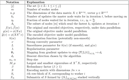
We will use the notation [j] ={i∈Z: 1≤i≤j}. All vector norms refer to 2-norm, and all matrix norms refer to spectral norm, unless otherwise noted. The superscript c will refer to complement of a subset, i.e., for A ⊆ [m], Ac = [m]\A. For a sequence of matrices {Mi}and a setAof indices, we will denote [Mi]i∈A to mean the matrix formed by stacking the matrices Mi vertically. The main notation used throughout the paper is provided in Table 1.
We consider a distributed computing network where the dataset {(xi, yi)}ni=1 is stored across a set ofm worker nodes, which directly communicate with a single master node. In practice the master node can be implemented using a fully-connected set of nodes, but this can still be abstracted as a single master node.
Notation Explanation
[j] The set{i∈Z: 1≤i≤j} m Number of worker nodes
n, p The dimensions of the data matrixX∈Rn×p, vectory∈Rn×1
kt Number of updates the master node waits for in iterationt, before moving on
ηt Fraction of nodes waited for in iteration,i.e.,ηt=kmt
At The subset of nodes [m] which send the fastestkt updates at iterationt
f(w),fe(w) The original and encoded objectives, respectively, under data parallelism g(w) =φ(Xw) The original objective under model parallelism
e
g(v) =φ(XS>v) The encoded objective under model parallelism
h(w) Regularization function (potentially non-smooth)
ν Strong convexity parameter
L Smoothness parameter forh(w) (if smooth), andg(w)
λ Regularization parameter
Ψt Mapping from gradient updates to step{∇fi(t)}i∈A
t 7→dt
dt Descent direction chosen by the algorithm
αt, α Step size
M, µ Largest and smallest eigenvalues ofX>X, respectively
β Redundancy factor (β≥1)
S Encoding matrix with dimensionsβn×n Si ith row-block ofS, corresponding to workeri
SA Submatrix ofS formed by{Si}i∈A⊆[m] stacked vertically
Table 1: Notation used in the paper.
2.1. Data parallelism
We focus on objectives of the form
f(w) = 1
2nkXw−yk
2+λh(w), (1)
whereX∈Rn×p and y∈Rn are the data matrix and data vector, respectively. We assume
each row ofX corresponds to a data sample, and the data samples and response variables can be horizontally partitioned as X =
X1>X2> · · · Xm>>
and y =
y1>y2> · · · ym>>
. In the uncoded setting, machinei stores the row-block Xi (Figure 1). We denote the largest and smallest eigenvalues of X>X withM >0, and µ≥0, respectively. We assumeλ≥0, andh(w)≥0 is a convex, extended real-valued function ofwthat does not depend on data. Sinceh(w) can take the valueh(w) =∞, this model covers arbitrary convex constraints on the optimization. Several important learning problems, such as ridge regression, LASSO, collaborative filtering (solved via alternating minimization), and support vector machine1 fall within this formulaton.
The encoding consists of solving the proxy problem
e
f(w) = 1
2nkS(Xw−y)k
2+λh(w) = 1 2n
m
X
i=1
kSi(Xw−y)k2
| {z }
fi(w)
+λh(w), (2)
instead, where S ∈ Rβn×n is a designed encoding matrix with redundancy factor β ≥ 1, partitioned as S = S1> S2> · · · Sm>> across m machines. Based on this partition, worker node i stores (SiX, Siy), and operates to solve the problem (2) in place of (1) (Figure 2). We will denote ˆw∈arg minfe(w), andw∗ ∈arg minf(w).
In general, the regularizer h(w) can be non-smooth. We will say thath(w) isL-smooth if∇h(w) exists everywhere and satisfies
h(w0)≤h(w) +h∇h(w), w0−wi+L
2kw
0−wk2
for someL >0, for allw, w0. The objectivef isν-strongly convex if, for allx, y,
f(y)≥f(x) +h∇f(x), y−xi+ ν
2kx−yk 2.
Once the encoding is done and appropriate data is stored in the nodes, the optimization process works in iterations. At iteration t, the master node broadcasts the current iterate
wtto the worker nodes, and wait forktgradient updates∇fi(w) to arrive, corresponding to that iteration, and then chooses a step directiondt and a step size αt (based on algorithm Ψt that maps the set of gradients updates to a step) to update the parameters. We will denote ηt = kmt. We will also drop the time dependence of k and η whenever it is kept constant.
The set of fastest kt nodes to send gradients for iteration t will be denoted as At. Once kt updates have been collected, the remaining nodes, denoted Act, are interrupted by the master node2. Algorithms 1 and 2 describe the generic mechanism of the proposed distributed optimization scheme at the master node and a generic worker node, respectively. The intuition behind the encoding idea is that waiting for onlykt< mworkers prevents the stragglers from holding up the computation, while the redundancy provided by using a tall matrixS compensates for the information lost by proceeding without the updates from stragglers (the nodes in the subset Act).
We next describe the three specific algorithms that we consider under data parallelism, to computedt.
Gradient descent. In this case, we assume that h(w) isL-smooth. Then we simply set the descent direction
dt=−
1 2nη
X
i∈At
∇fi(wt) +λ∇h(wt)
!
.
We keepkt=kconstant, chosen based on the number of stragglers in the network, or based on the desired operating regime.
Limited-memory-BFGS. We assume that h(w) = kwk2, and assume µ+λ > 0. Al-though L-BFGS is traditionally a batch method, requiring updates from all nodes, its stochastic variants have also been proposed by Mokhtari and Ribeiro (2015); Berahas et al. (2016). The key modification to ensure convergence in this case is that the Hessian estimate must be computed via gradient components that are common in two consecutive iterations,
i.e., from the nodes inAt∩At−1. We adapt this technique to our scenario. Fort >0, define
ut:=wt−wt−1, and3
rt:=
m
2n|At∩At−1|
X
i∈At∩At−1
(∇fi(wt)− ∇fi(wt−1)).
Then once the gradient terms{∇fi(wt)}i∈At are collected, the descent direction is computed
by dt = −Btegt, where egt =
1 2ηn
P
i∈At∇fi(wt), and Bt is the inverse Hessian estimate for
iterationt, which is computed by
Bt(`+1)=Vj>`,tBt(`)Vj`,t+ρj`,tuj`,tu
>
j`,t, ρj =
1
r>j uj
, Vj =I−ρjrju>j
with j`,t = t−eσ +`, B
(0) t =
r> t rt
r>
t utI, and Bt := B
(σe)
t with eσ := min{t, σ}, where σ is
the L-BFGS memory length. Once the descent direction dt is computed, the step size is determined through exact line search4. To do this, each worker node computesSiXdt, and sends it to the master node. Once again, the master node only waits for the fastestktnodes, denoted by Dt ⊆[m] (where in general Dt 6=At), to compute the step size that minimizes the function along dt, given by
αt=−ρ
d>tegt
d>t XeD>XeDdt
, (3)
whereXeD = [SiX]i∈D
t, and 0< ρ <1 is a back-off factor of choice.
Proximal gradient. Here, we consider the general case of non-smoothh(w)≥0, λ≥0. The descent direction dt is given by
dt= arg min w
e
Ft(w)−wt,
where
e
Ft(w) :=
1 2ηn
X
i∈At
fi(wt) +
*
1 2ηn
X
i∈At
∇fi(wt), w−wt
+
+λh(w) + 1
2αkw−wtk
2.
We keep the step sizeαt=α and kt=k constant.
3. Note that we assume here that the intersectionAt∩At−1is non-empty. This can be ensured by adaptively
choosingkt (waiting for sufficiently many workers) so thatAt∩At−16=∅. This is further discussed in
Section 3. However, our experiments indicate that convergence is still possible even when this condition does not hold.
Algorithm 1 Generic encoded distributed optimization procedure under data parallelism, at the master node.
1: Given: Ψt, a sequence of functions that map gradients {∇fi(wt)}i∈At to a descent
directiondt
2: Initialize w0,α0
3: fort= 1, . . . , T do
4: broadcast wtto all worker nodes
5: wait to receive kt gradient updates {∇fi(wt)}i∈At 6: send interrupt signal to the nodes in Act
7: compute the descent direction dt= Ψt {∇fi(wt)}i∈At
8: determine step sizeαt
9: take the stepwt+1=wt+αtdt
10: end for
Algorithm 2 Generic encoded distributed optimization procedure under data parallelism, at worker node i.
1: Given: fi(w) =kSi(Xw−y)k2
2: fort= 1, . . . , T do
3: wait to receive wt
4: while not interrupted by masterdo
5: compute∇fi(wt)
6: end while
7: if computation was interrupted then
8: continue
9: else
10: send∇fi(wt)
11: end if
12: end for
2.2. Model parallelism
Under the model parallelism paradigm, we focus on objectives of the form
ming(w) := min
w φ(Xw) = minw φ m
X
i=1
Xiwi
!
, (4)
where the data matrix is partitioned as X = [X1X2 · · · Xm], the parameter vector is partitioned as w =
w>1 w2> · · · w>m>
, φ is convex, and g(w) is L-smooth. Note that the data matrix X is partitioned horizontally, meaning that the dataset is split across features, instead of data samples (see Figure 3). This class of objectives is applicable to any classification or regression problem with generalized linear models, such as logistic regression, softmax regression, and multinomial regression.
We encode the problem (4) by settingw=S>v, and solving the problem
min
v eg(v) :=φ
XS>v
= min v φ
m
X
i=1
XSi>vi
!
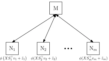
N1 N2 Nm M
φ(X1w1+z1) φ(X2w2+z2) φ(Xmwm+zm)
Figure 3: Uncoded distributed optimiza-tion with model parallelism, where ith node stores theith partition of the model
wi. Fori= 1, . . . , m,zi =Pj6=iXjwj.
N1 N2 Nm
M
φ XS> 1v1+ ˜z1
φ(XS>
2v2+ ˜z2) φ(XSm>vm+ ˜zm)
Figure 4: Encoded setup with model par-allelism, where ith node stores the par-tition vi of the model in the “lifted” space. For i = 1, . . . , m, zei = Pj6=iuj =
P
j6=iXS > j vj.
where w ∈ Rp and S> =
S1>S2> · · · Sm>
∈ Rp×βp (see Figure 4). As a result, worker i stores the column-block XSi>, as well as the iterate partition vi. Note that we increase the dimensions of the parameter vector by multiplying the datasetX with a wide encoding matrix S> from the right, and as a result we have redundant coordinates in the system. As in the case of data parallelism, such redundant coordinates provide robustness against erasures arising due to stragglers. Such increase in coordinates means that the problem is simply lifted onto a larger dimensional space, while preserving the original geometry of the problem. We will denoteui,t =XSi>vi,t, wherevi,t is the parameter iterates of workeriat iterationt. In order to compute updates to its parametersvi, worker ineeds the up-to-date value of ezi:=Pj6=iuj, which is provided by the master node at every iteration.
Let S= arg minwg(w), and given w, letw∗ be the projection of wonto S. We will say thatg(w) satisfiesν-restricted-strong convexity (Lai and Yin (2013)) if
h∇g(w), w−w∗i ≥νkw−w∗k2
for allw. Note that this is weaker than (implied by) strong convexity sincew∗ is restricted to be the projection ofw, but unlike strong convexity, it is satisfied under the case whereφ
is strongly convex, butX has a non-trivial null space,e.g., when it has more columns than rows.
For a given w ∈Rp, we define the level set ofg at w asD
g(w) :={w0 :g(w0)≤g(w)}. We will say that the level set at w0 has diameterR if
supkw−w0k:w, w0 ∈Dg(w0) ≤R.
As in the case of data parallelism, we assume that the master node waits for kupdates at every iteration, and then moves onto the next iteration (see Algorithms 3 and 4). We similarly defineAt as the set of kfastest nodes in iterationt, and also define
Ii,t =
Algorithm 3 Encoded block coordinate descent at worker nodei.
1: Given: Xi,vi.
2: fort= 1, . . . , T do
3: wait to receive (Ii,t−1,zei,t)
4: if Ii,t == 1then
5: take stepvi,t=vi,t−1+di,t−1
6: else
7: setvi,t =vi,t−1
8: end if
9: while not interrupted by masterdo
10: compute next stepdi,t =αSiX>∇φ XSi>vi,t+zei,t
11: computeui,t =XSi>vi,t
12: end while
13: if computation was interrupted then
14: continue
15: else
16: sendui,t to master node
17: end if
18: end for
Algorithm 4 Encoded block coordinate descent at the master node.
1: fort= 1, . . . , T do
2: for i= 1, . . . , mdo
3: send (Ii,t−1,zei,t) to workeri
4: end for
5: wait to receive kupdated parameters {ui,t}i∈At
6: send interrupt signal to the nodes in Act
7: set ui,t =ui,t−1 fori∈Act
8: compute ezi,t = P
j6=iuj,t for all i
9: end for
Under model parallelism, we consider block coordinate descent, described in Algo-rithm 3, where worker istores the current values of the partitionvi, and performs updates on it, given the latest values of the rest of the parameters. The parameter estimate at time
t is denoted by vi,t, and we also define ezi,t = P
j6=iui,t = Pj6=iXSj>vj. The iterates are updated by
vi,t−vi,t−1 = ∆i,t:=
−α∇ieg(vt−1), ifi∈At 0, otherwise,
for a step size parameterα >0, where∇irefers to gradient only with respect to the variables
vi,i.e.,∇eg= [∇ieg]i∈[m]. Note that ifi /∈Atthenvi does not get updated in workeri, which
3. Main Theoretical Results: Convergence Analysis
In this section, we prove convergence results for the algorithms described in Section 2. Note that since we modify the original optimization problem and solve it obliviously to this change, it is not obvious that the solution has any optimality guarantees with respect to the original problem. We show that, it is indeed possible to provide convergence guarantees in terms of theoriginal objective under the encoded setup.
3.1. A spectral condition
In order to show convergence under the proposed framework, we require the encoding matrix
S to satisfy a certain spectral criterion on S. LetSAdenote the submatrix ofS associated with the subset of machinesA,i.e.,SA= [Si]i∈A. Then the criterion in essence requires that for any sufficiently large subsetA,SAbehaves approximately like a matrix with orthogonal columns. We make this precise in the following statement.
Definition 1 Let β ≥1, and 1β ≤η ≤1 be given. A matrix S ∈ Rβn×n is said to satisfy
the (m, η, )-block-restricted isometry property ((m, η, )-BRIP) if for any A ⊆ [m] with
|A| ≥ηm,
(1−)In 1
ηS
>
ASA(1 +)In. (6)
Note that this is similar to the restricted isometry property used in compressed sensing (Candes and Tao (2005)), except that we do not require (6) to hold for every submatrix of
Sof sizeRηn×n. Instead, (6) needs to hold only for the submatrices of the formSA= [Si]i∈A, which is a less restrictive condition. In general, it is known to be difficult to analytically prove that a structured, deterministic matrix satisfies the general RIP condition. Such diffi-culty extends to the BRIP condition as well. However, it is known that i.i.d. sub-Gaussian ensembles and randomized Fourier ensembles satisfy this property (Candes and Tao (2006)). In addition, numerical evidence suggests that there are several families of constructions for
S whose submatrices have eigenvalues that mostly tend to concentrate around 1. We point out that although the strict BRIP condition is required for the theoretical analysis, in prac-tice the algorithms perform well as long as the bulk of the eigenvalues of SA lie within a small interval (1−,1 +), even though the extreme eigenvalues may lie outside of it (in the non-adversarial setting). In Section 4, we explore several classes of matrices and discuss their relation to this condition.
3.2. Convergence of encoded gradient descent
We first consider the algorithms described under data parallelism architecture. The follow-ing theorem summarizes our results on the convergence of gradient descent for the encoded problem.
Theorem 2 Let wt be computed using encoded gradient descent with an encoding matrix
that satisfies (m, η, )-BRIP, with step size αt = M(1+2ζ)+λL for some 0 < ζ ≤ 1, for all
t. Let {At} be an arbitrary sequence of subsets of [m] with cardinality |At| ≥ ηm for all t.
1.
1
t
t
X
τ=1
f(wτ)−κ1f(w∗)≤
4f(w0) +21αkw0−w∗k2 (1−7)t
2. If f is in additionν-strongly convex, then
f(wt)−
κ2
2(κ2−γ) 1−κ2γ
f(w∗)≤(κ2γ)tf(w0), t= 1,2, . . . ,
where κ1 = 1+31−7, κ2 =
1+
1−, and γ =
1−M4(1+νζ(1−ζ)+λL) , where is assumed to be small
enough so that κ2γ <1.
The proof is provided in Appendix A, which relies on the fact that the solution to the effective “instantaneous” problem corresponding to the subset At lies in a bounded set {w : f(w) ≤ κf(w∗)} (where κ depends on the encoding matrix and strong convexity assumption on f), and therefore each gradient descent step attracts the iterate towards a point in this set, which must eventually converge to this set. Theorem 2 shows that encoded gradient descent can achieve the standardO 1tconvergence rate for the general case5, and linear convergence rate for the strongly convex case, up to an approximate minimum. For the convex case, the convergence is shown on the running mean of past function values, whereas for the strongly convex case we can bound the function value at every step. Note that although the nodes actually minimize the encoded objective fe(w), the convergence
guarantees are given in terms of the original objective f(w). Note that under the strongly convex case, linear convergence requires conditionκ2γ <1. Sinceγ, which is slightly smaller than 1, is a decreasing function of the fraction of the strong convexity parameter to the smoothness parameter, the practical implication of this is that the less the curvature of the function (the smaller the strong convexity parameter ν), the more workers we need to wait in each iteration, so that κ2 is small enough to satisfy κ2γ < 1, which ensures the linear convergence guarantee of the theorem. Note that even if this condition is not satisfied, the algorithm can still converge, but not necessarily at the linear rate promised by the theorem. Theorem 2 provides deterministic, sample path convergence guarantees under any (ad-versarial) sequence of active nodes {At}, which is in contrast to the stochastic methods, which show convergence typically in expectation. Further, the convergence rate is not af-fected by the tail behavior of the delay distribution, since the delayed updates of stragglers are not applied to the iterates.
Note that since we do not seek exact solutions under data parallelism, we can keep the redundancy factor β fixed regardless of the number of stragglers. Increasing number of stragglers in the network simply results in a looser approximation of the solution, allowing for a graceful degradation. This is in contrast to existing work Tandon et al. (2017) seeking exact convergence under coding, which shows that the redundancy factor must grow linearly with the number of stragglers.
3.3. Convergence of encoded L-BFGS
We consider the variant of L-BFGS described in Section 2. For our convergence result for L-BFGS, we need another assumption on the matrix S, in addition to (6). Defining
˘
St= [Si]i∈At∩At−1 fort >0, we assume that for someδ >0,
δI S˘t>S˘t (7)
for all t > 0. Note that this requires that one should wait for sufficiently many nodes to send updates so that the overlap set At∩At−1 has more than 1β nodes, and thus the matrix ˘St can be full rank. When the columns of X are linearly independent, this is satisfied if η≥ 12+21β in the worst-case, and in the case where node delays are i.i.d. across machines, it is satisfied in expectation ifη ≥ √1
β. One can also choosektadaptively so that
kt= min
n
k:|At(k)∩At−1|> β1
o
. We note that although this condition is required for the theoretical analysis, the algorithm may perform well in practice even when this condition is not satisfied.
We first show that this algorithm results in stable inverse Hessian estimates under the proposed model, under arbitrary realizations of{At}(of sufficiently large cardinality), which is done in the following lemma.
Lemma 3 Let µ+λ > 0. Then there exist constants c1, c2 > 0 such that for all t, the
inverse Hessian estimate Bt satisfiesc1I Btc2I.
The proof, provided in Appendix A, is based on the well-known trace-determinant method. Using Lemma 3, we can show the following convergence result.
Theorem 4 Let µ+λ >0, and let wt be computed using the L-BFGS method described in
Section 2, with an encoding matrix that satisfies (m, η, )-BRIP. Let {At},{Dt}be arbitrary
sequences of subsets of[m]with cardinality|At|,|Dt| ≥ηmfor allt. Then, forf as described
in Section 2,
f(wt)−
κ2(κ−γ)
1−κγ f(w
∗
)≤(κγ)tf(w0),
where κ = 1+1−, and γ = 1− 4(µ+λ)c1c2
(M+λ)(1+)(c1+c2)2
, where c1 and c2 are the constants in
Lemma 3.
Similar to Theorem 2, the proof is based on the observation that the solution of the effective problem at timetlies in a bounded set around the true solutionw∗. As in gradient descent, coding enables linear convergence deterministically, unlike the stochastic and multi-batch variants of L-BFGS,e.g., Mokhtari and Ribeiro (2015); Berahas et al. (2016).
3.4. Convergence of encoded proximal gradient
Theorem 5 Let wt be computed using encoded proximal gradient with an encoding matrix
that satisfies (m, η, )-BRIP, with step size αt = α < M1 , and where < 17. Let {At} be
an arbitrary sequence of subsets of [m] with cardinality |At| ≥ηm for all t. Then, forf as
described in Section 2,
1. For all t,
1
t
t
X
τ=1
f(wτ)−κf(w∗)≤
4f(w0) +21αkw0−w∗k2 (1−7)t ,
2. For all t,
f(wt+1)≤κf(wt),
where κ= 1+71−3.
As in the previous algorithms, the convergence guarantees hold for arbitrary sequences of active nodes {At}. Note that as in the gradient descent case, the convergence is shown on the mean of past function values. Since this does not prevent the iterates from having a sudden jump at a given iterate, we include the second part of the theorem to complement the main convergence result, which implies that the function value cannot increase by more than a small factor of its current value.
3.5. Convergence of encoded block coordinate descent
Finally, we consider the convergence of encoded block coordinate descent algorithm. The following theorem characterizes our main convergence result for this case.
Theorem 6 Let wt = S>vt, where vt is computed using encoded block coordinate descent
as described in Section 2. LetS satisfy (m, η, )-BRIP, and the step size satisfyα < L(1+1 ).
Let {At}be an arbitrary sequence of subsets of [m]with cardinality|At| ≥ηmfor all t. Let
the level set of g at the first iterate Dg(w0) have diameter R. Then, for g(w) =φ(Xw) as
described in Section 2, the following hold.
1. If φ is convex, then
g(wt)−g(w∗)≤
1 1 π0 +Ct
,
where π0 =g(w0)−g(w∗), andC = (1−R2)α
1−αL20.
2. If g is ν-restricted-strongly convex, then
g(wt)−g(w∗)≤
1−1
ξ
t
(g(w0)−g(w∗)),
where ξ = ν(1−2 )α
Theorem 6 demonstrates that the standard O 1t
rate for the general convex, and linear rate for the strongly convex case can be obtained under the encoded setup. Similar to the previous cases, encoding allows for deterministic convergence guarantees under adversarial failure patterns.
Note that unlike the data parallelism setup, we can achieve exact minimum under model parallelism, since the underlying geometry of the problem does not change under encoding; the same objective is simply mapped onto a higher-dimensional space, which has redundant coordinates. In every iteration, such redundancy serves as a “soft” error correction mecha-nism, by allowing each worker to receive sufficient information about the up-to-date values of the rest of the parameters hosted in the other nodes, even though a subset of them are not able to send their updates sufficiently fast. The smaller theis in the BRIP condition, the more representative the redundant coordinates are for the missing ones, which is reflected in the convergence rate, as a non-zero slightly weakens the constants in the convergence expressions. Still, note that this penalty in convergence rate only depends on the encoding matrix and not on the delay profile in the system. This is in contrast to the asynchronous coordinate descent methods; for instance, in Liu et al. (2015), the step size is required to shrinkexponentially in the maximum allowable delay, and thus the guaranteed convergence rate can exponentially degrade with increasing worst-case delay in the system. The same is true for the linear convergence guarantee in Peng et al. (2016).
4. Code Design
4.1. Block RIP condition and code design
We first discuss two classes of encoding matrices with regard to the BRIP condition; namely equiangular tight frames, and random matrices.
Tight frames. A unit-norm frame for Rn is a set of vectors F ={ai}nβi=1 with kaik = 1, whereβ ≥1, such that there exist constants ξ2 ≥ξ1 >0 such that, for anyu∈Rn,
ξ1kuk2 ≤
nβ
X
i=1
|hu, aii|2 ≤ξ2kuk2.
The frame is tight if the above is satisfied withξ1 =ξ2. In this case, it can be shown that the constants are equal to the redundancy factor of the frame, i.e., ξ1 = ξ2 = β. If we form S∈R(βn)×n by rows that form atight frame, then we haveS>S=βI, which ensures kXw−yk2 = 1
βkSXw−Syk
2. Then for any solution ˆw to the encoded problem (with
k=m),
∇fe( ˆw) =X>S>S(Xwˆ−y) =βX>(Xwˆ−y) =β∇f( ˆw).
Therefore, the solution to the encoded problem satisfies the optimality condition for the original problem as well:
−∇fe( ˆw)∈∂h( ˆw), ⇔ −∇f( ˆw)∈∂h( ˆw),
and if f is also strongly convex, then ˆw =w∗ is the unique solution. This means that for
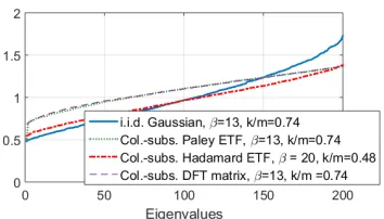
Figure 5: Sample spectrum of SA>SA for various constructions with high redun-dancy, and small k(normalized).
Figure 6: Sample spectrum of SA>SA for various constructions with moderate re-dundancy, and largek(normalized).
Define the maximal inner product of a unit-norm tight frame F ={ai}nβi=1, where ai ∈ Rn,∀i, by
ω(F) := max ai,aj∈F
i6=j
|hai, aji|.
Definition 7 (Equiangular tight frame (ETF)) A tight frame is called an equiangular tight frame (ETF) if |hai, aji|=ω(F) for everyi6=j.
Proposition 8 (Welch (1974)) Let F = {ai}inβ=1 be a tight frame, where ai ∈ Rn for
i= 1, . . . , nβ. Then ω(F)≥qnβ−β−11. Moreover, equality is satisfied if and only if F is an
equiangular tight frame.
Therefore, an ETF minimizes the correlation between its individual elements, making each submatrix SA>SA as close to orthogonal as possible. This, combined with the property that tight frames preserve the optimality condition when all nodes are waited for (k=m), make ETFs good candidates for encoding, in light of the required property (6). We specifically evaluate the Paley ETF from Paley (1933) and Goethals and Seidel (1967); Hadamard ETF from Sz¨oll˝osi (2013) (not to be confused with Hadamard matrix); and Steiner ETF from Fickus et al. (2012) in our experiments.
Although the derivation of tight eigenvalue bounds for subsampled ETFs is a long-standing problem, numerical evidence (see Figures 5, 6) suggests that they tend to have their eigenvalues more tightly concentrated around 1 than random matrices (also supported by the fact that they satisfy Welch bound, Proposition 8 with equality).
Random matrices. Another natural choice of encoding could be to use i.i.d. random matrices. Although encoding with such random matrices can be computationally expensive and may not have the desirable properties of encoding with tight frames, their eigenvalue behavior can be characterized analytically. In particular, using the existing results on the eigenvalue scaling of large i.i.d. Gaussian matrices from Geman (1980); Silverstein (1985) and union bound, it can be shown that
P max
A:|A|=kλmax
1
βηnS
> ASA
>
1 +
r
1
βη
2!
P min A:|A|=kλmin
1
βηnS
> ASA
<
1−
r
1
βη
2!
→0, (9)
as n → ∞, if the elements of SA are drawn i.i.d. from N(0,1). Hence, for sufficiently large redundancy and problem dimension, i.i.d. random matrices are good candidates for encoding as well. However, for finite β, even if k = m, in general the optimum of the original problem is not recovered exactly, for such matrices.
4.2. Discussion on required redundancy
A common problem with worst-case bounds is that they are often pessimistic when com-pared against actual performance on real instances. In our case, directly computing the redundancy for small enough < 1 (as required by Theorem 5, for instance) suggests a required redundancyβ of more than 200. However, as we also show in Section 5, in practice much lower values values of redundancy (such as β = 2) results in good performance. The reason for this apparent discrepancy is that in the proofs of the theorems, we take a conservative approach and bound quadratic terms of the form
ξ(w) =
(Xw−y)>(SA>SA−I)(Xw−y)
kXw−yk2 , which is at worst
ξ(w)≤= maxnλmax
SA>SA−I
,−λmin
SA>SA−I
o .
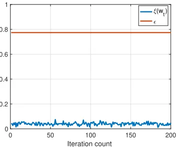
Note that the inequality is tight ifXw−y is an extremal eigenvector ofSATSA−I, which, although possible, is highly unlikely. We illustrate this point through an example experiment shown in Figure 7, which plotsξ(wt) for a run of gradient descent on linear regression with random data, wherewt is thetthiterate. In the entire optimization process, it is clear that
is a very pessimistic upper bound on ξ(wt).
In particular, most of the energy of the vector Xwt−y lies in the eigenspace associated with the bulk of the eigenvalues of SA>SA. From another perspective, if we were to use the “empirical” maximum of the value for this particular run (instead of the worst-case bound, the largest eigenvalue), we would achieve= 0.074 at redundancyβ= 2, a dramatic improvement compared to the above requirement ofβ >200 for= 17.
This observation implies that for good practical performance, what is more important is to ensure that most eigenvalues lie close to, or is exactly 1. The following proposition shows that for ETFs, the bulk of the eigenvalues can be identically 1.
Proposition 9 If the rows of S are chosen to form an ETF with redundancy β, then for
η≥1− 1β, 1βSA>SA has n(1−β(1−η)) eigenvalues equal to 1.
This follows immediately from Cauchy interlacing theorem, using the fact that SASA> and
0 50 100 150 200
Iteration count
0 0.2 0.4 0.6 0.8 1
(wt)
Figure 7: The evolution of ξ(wt) and against iteration count. The parameters are
(n, d, β) = (2001,1400,2), where we encode the data variables with a Paley ETF. We
initialize the elements ofw0 with a standard normal distribution. We set η = 0.9,i.e., we wait for 90% of the machines at every step.
4.3. Efficient encoding
In this section we discuss some of the possible practical approaches to encoding. Some of the practical issues involving encoding include the computational complexity of encoding, as well as the loss of sparsity in the data due to the multiplication withS, and the resulting increase in time and space complexity. We address these issues in this section.
4.3.1. Efficient distributed encoding with sparse matrices
Let the dataset (X, y) lie in a database, accessible to each worker node, where each node is responsible for computing their own encoded partitions SiX and Siy. We assume that
S has a sparse structure. Given S, defineBi(S) ={j:Sij 6= 0} as the set of indices of the non-zero elements of theith row ofS. For a setI of rows, we defineBI(S) =∪i∈IBi(S).
Let us partition the set of rows of S, [βn], into m machines, and denote the partition of machine k asIk, i.e., Fm
k=1Ik = [βn], where t denotes disjoint union. Then the set of non-zero columns ofSk is given byBIk(S). Note that in order to computeSkX, machinek
only requires the rows ofXin the setBIk(S). In what follows, we will denote this submatrix
of X byXek,i.e., if x>i is the ith row of X,Xek:=
x>i i∈B
Ik(S). Similarlyyek = [yi]i∈BIk(S),
whereyi is the ith element ofy.
Consider the specific computation that needs to be done by worker k during the it-erations, for each algorithm. Under the data parallelism setting, worker k computes the following gradient:
∇fk(w) =X>Sk>Sk(Xw−y) (a)
= Xek>Sk>Sk(Xekw−yek) (10)
where (a) follows since the rows ofXthat are not inBIk get multiplied by zero vector. Note
that the last expression can be computed without any matrix-matrix multiplication. This gives a natural storage and computation scheme for the workers. Instead of computing
can store Xek in uncoded form, and compute the gradient through (10) whenever needed,
using only matrix-vector multiplications. Since Sk is sparse, the overhead associated with multiplications of the formSkv andSk>v is small.
Similarly, under model parallelism, the computation required by workerk is
∇keg(v) =SkX>∇kφ
XSk>vk+ezk
=SkXek>∇kφ
e
XkSk>vk+ezk
, (11)
and as in the data parallelism case, the worker can store Xek uncoded, and compute (11)
online through matrix-vector multiplications.
Example: Steiner ETF. We illustrate the described technique through Steiner ETF, based on the construction proposed in Fickus et al. (2012), using (2,2, v)-Steiner systems. Let v be a power of 2, let H ∈ Rv×v be a real Hadamard matrix, and let hi be the ith column ofH, fori= 1, . . . , v. Consider the matrixV ∈ {0,1}v×v(v−1)/2, where each column is the incidence vector of a distinct two-element subset of{1, . . . , v}. For instance, forv= 4,
V =
1 1 1 0 0 0 1 0 0 1 1 0 0 1 0 1 0 1 0 0 1 0 1 1
.
Note that each of the v rows have exactlyv−1 non-zero elements. We construct Steiner ETF S as a v2×v(v−21) matrix by replacing each 1 in a row with a distinct column of H, and normalizing by √v−1. For instance, for the above example, we have
S= √1
3
h2 h3 h4 0 0 0
h2 0 0 h3 h4 0
0 h2 0 h3 0 h4 0 0 h2 0 h3 h4
.
We will call a set of rows of S that arises from the same row ofV a block. In general, this procedure results in a matrix S with redundancy factorβ = v−2v1. In full generality, Steiner ETFs can be constructed for larger redundancy levels; we refer the reader to Fickus et al. (2012) for a full discussion of these constructions.
We partition the rows of the V matrix into m machines, so that each machine gets assigned mv rows of V, and thus the corresponding mv blocks ofS.
This construction and partitioning scheme is particularly attractive for our purposes for two reasons. First, it is easy to see that for any node k, |BIk| is upper bounded by
v(v−1)
m =
2n
m, which means the memory overhead compared to the uncoded case is limited to a factor6 of β. Second, each block of S
k consists of (almost) a Hadamard matrix, so the multiplication Skv can be efficiently implemented through Fast Walsh-Hadamard Transform.
Example: Haar matrix. Another possible choice of sparse matrix is column-subsampled Haar matrix, which is defined recursively by
H2n=
1 √ 2
Hn⊗[1 1]
In⊗[1 −1]
, H1= 1,
where ⊗ denotes Kronecker product. Given a redundancy level β, one can obtain S by randomly sampling nβ columns of Hn. It can be shown that in this case, we have |BIk| ≤
βnlog(n)
m , and hence encoding with Haar matrix incurs a memory cost by logarithmic factor.
4.3.2. Fast transforms
Another computationally efficient method for encoding is to use fast transforms: Fast Fourier Transform (FFT), ifS is chosen as a subsampled DFT matrix, and the Fast Walsh-Hadamard Transform (FWHT), ifS is chosen as a subsampled real Hadamard matrix. In particular, one can insert rows of zeroes at random locations into the data pair (X, y), and then take the FFT or FWHT of each column of the augmented matrix. This is equivalent to a randomized Fourier or Hadamard ensemble, which is known to satisfy the RIP with high probability by Candes and Tao (2006). However, such transforms do not have the memory advantages of the sparse matrices, and thus they are more useful for the setting where the dataset is dense, and the encoding is done offline.
4.4. Cost of encoding
Since encoding increases the problem dimensions, it clearly comes with the cost of increased space complexity. The memory and storage requirement of the optimization still increases by a factor of 2, if the encoding is done offline (for dense datasets), or if the techniques described in the previous subsection are applied (for sparse datasets)7. Note that the added redundancy can come by increasing the amount of effective data points per machine, by increasing the number of machines while keeping the load per machine constant, or a combination of the two. In the first case, the computational load per machine increases by a factor of β. Although this can make a difference if the system is bottlenecked by the computation time, distributed computing systems are typically communication-limited, and thus we do not expect this additional cost to dominate the speed-up from the mitigation of stragglers.
5. Numerical Results
We implement the proposed technique on four problems: ridge regression, matrix factoriza-tion, logistic regression, and LASSO.
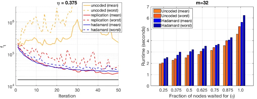
Figure 8: Left: Sample evolution of uncoded, replication, and Hadamard (FWHT)-coded cases, for k = 12, m = 32. Right: Runtimes of the schemes for different values of η, for the same number of iterations for each scheme. Note that this essentially captures the delay profile of the network, and does not reflect the relative convergence rates of different methods.
5.1. Data parallelism
5.1.1. Ridge regression
We generate the elements of matrixX i.i.d. ∼N(0,1), and the elements ofy are generated from X and an i.i.d. N(0,1) parameter vector w∗, through a linear model with Gaussian noise, for dimensions (n, p) = (4096,6000). We solve the problem minw 21nkS(Xw−y)k2+
λ
2kwk2, for regularization parameterλ= 0.05. We evaluate column-subsampled Hadamard matrix with redundancy β = 2 (encoded using FWHT), replication and uncoded schemes. We implement distributed L-BFGS as described in Section 3 on an Amazon EC2 cluster using mpi4py Python package, over m = 32 m1.small instances as worker nodes, and a single c3.8xlargeinstance as the central server.
Figure 8 shows the result of our experiments, which are aggregated from 20 trials. In addition to uncoded scheme, we consider data replication, where each uncoded partition is replicated β = 2 times across nodes, and the server discards the duplicate copies of a partition, if received in an iteration. It can be seen that for lowη, uncoded L-BFGS may not converge when a fixed number of nodes are waited for, whereas the Hadamard-coded case stably converges. We also observe that the data replication scheme converges on average, but its performance may deteriorate if both copies of a partition are delayed. Figure 8 suggests that this performance can be achieved with an approximately 40% reduction in the runtime, compared to waiting for all the nodes.
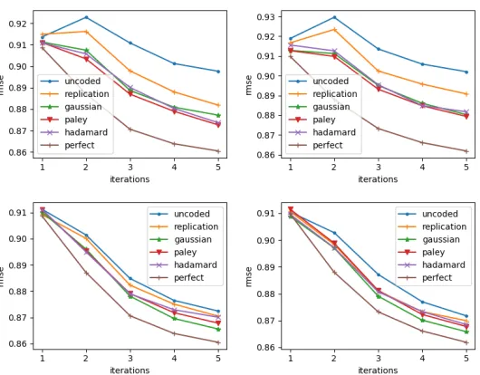
Figure 9: Test RMSE for m= 8 (left) andm = 24 (right) nodes, where the server waits for k=m/8 (top) and k=
m/2 (bottom) responses. “Perfect” refers to the case where
k=m.
Figure 10: Total runtime with
m = 8 and m = 24 nodes for different values ofk, under fixed 100 iterations for each scheme.
less accurate solutions, as can be seen from the aggregated sample evolution on the left. The left plot shows that, encoding effectively counteracts this effect, maintaining smooth convergence due to the redundant data in the nodes.
5.1.2. Matrix factorization
We next apply matrix factorization on the MovieLens-1M dataset (Riedl and Konstan (1998)) for the movie recommendation task. We are given R, a sparse matrix of movie ratings 1–5, of dimension #users×#movies, where Rij is specified if user i has rated movie j. We withhold randomly 20% of these ratings to form an 80/20 train/test split. The goal is to recover user vectors xi ∈ Rp and movie vectors yi ∈ Rp (where p is the
embedding dimension) such that Rij ≈ xTi yj +ui +vj +b, where ui, vj, and b are user, movie, and global biases, respectively. The optimization problem is given by
min xi,yj,ui,vj
X
i,j: observed
(Rij−ui−vj−xTi yj−b)2+λ
X
i
kxik22+kuk22+
X
j
kyjk22+kvk22
.
(12) We chooseb= 3,p= 15, andλ= 10, which achieves test RMSE 0.861, close to the current best test RMSE on this dataset using matrix factorization8.
Problem (12) is often solved using alternating minimization, minimizing first over all (xi, ui), and then all (yj, vj), in repetition. Each such step further decomposes by row and column, made smaller by the sparsity of R. To solve for (xi, ui), we first extract
Ii ={j|rij is observed}, and minimize
yIT
i,1
xi
ui
−(RTi,Ii−vIi−b1)
2
+λ X
i
kxik22+kuk22
!
(13)
for each i, which gives a sequence of regularized least squares problems with variable w= [xTi , ui]T, which we solve distributedly using coded L-BFGS; and repeat for w= [yTj, vj]T, for all j.
The Movielens experiment is run on a single 32-core machine with Linux 4.4. In or-der to simulate network latency, an artificial delay of ∆ ∼ exp(10 ms) is imposed each time the worker completes a task. Small problem instances (n < 500) are solved locally at the central server, using the built-in function numpy.linalg.solve. To reduce over-head, we create a bank of encoding matrices {Sn} for Paley ETF and Hadamard ETF, for n = 100,200, . . . ,3500, and then given a problem instance, subsample the columns of the appropriate matrix Sn to match the dimensions. Overall, we observe that encoding overhead is amortized by the speed-up of the distributed optimization.
Figure 9 gives the final performance of our distributed L-BFGS for various encoding schemes, for each of the 5 epochs, which shows that coded schemes are most robust for small k. A full table of results is given in Appendix D.
5.1.3. LASSO
We solve the LASSO problem, with the objective
min w
1
2nkXw−yk
2+λkwk 1,
where X ∈ R130,000×100,000 is a matrix with i.i.d. N(0,1) entries, and y is generated from
X and a parameter vector w∗ through a linear model with Gaussian noise:
y=Xw∗+σz,
where σ = 40, z ∼ N(0,1). The parameter vector w∗ has 7695 non-zero entries out of 100,000, where the non-zero entries are generated i.i.d. from N(0,4). We choose λ = 0.6 and consider the sparsity recovery performance of the corresponding LASSO problem, solved using proximal gradient (iterative shrinkage/thresholding algorithm).
We implement the algorithm over 128 t2.medium worker nodes which collectively store the matrix X, and a c3.4xlarge master node. We measure the sparsity recovery perfor-mance of the solution using the F1 score, defined as the harmonic mean
F1 = 2P R
P +R,
whereP andR are precision recall of the solution vector ˆwrespectively, defined as
P = |{i:w
∗
i 6= 0,wˆi 6= 0}| |i: ˆwi 6= 0|
, R= |{i:w
∗
0 10 20 30 40 50 60 Seconds (s)
0.3 0.4 0.5 0.6 0.7 0.8 0.9
F1 sparsity recovery
Uncoded (k=80) Steiner (k=80) Uncoded (k=128) Replication (k=128)
Figure 11: Evolution of F1 sparsity recovery performance for each scheme.
Figure 11 shows the sample evolution of the F1 score of the model under uncoded, replication, and Steiner encoded scenarios, with artificial multi-modal communication delay distribution q1N(µ1, σ12) +q2N(µs, σ22) +q3N(µ3, σ32), where q1 = 0.8, q2 = 0.1, q3 = 0.1;
µ1 = 0.2s, µs = 0.6s, µ3 = 1s; and σ1 = 0.1s, σ = 0.2s, σ3 = 0.4s, independently at each node. We observe that the uncoded case k = 80 results in a performance loss in sparsity recovery due to data dropped from delayed noes, and uncoded and replication with
k= 128 converges slow due to stragglers, while Steiner coding withk= 80 is not delayed by stragglers, while maintaining almost the same sparsity recovery performance as the solution of the uncoded k= 128 case.
5.2. Model parallelism
5.2.1. Logistic regression
In our next experiment, we apply logistic regression for document classification for Reuters Corpus Volume 1 (rcv1.binary) dataset from Lewis et al. (2004), where we consider the binary task of classifying the documents into corporate/industrial/economics vs. gov-ernment/social/markets topics. The dataset has 697,641 documents, and 47,250 term frequency-inverse document frequency (tf-idf) features. We randomly select 32,500 fea-tures for the experiment, and reserve 100,000 documents for the test set. We use logistic regression with`2-regularization for the classification task, with the objective
min w,b
1
n
n
X
i=1
log1 + expn−zi>w+bo+λkwk2,
wherezi=yixi is the data sample xi multiplied by the labelyi ∈ {−1,1}, andb is the bias variable. We solve this optimization using encoded distributed block coordinate descent as described in Section 2, and implement Steiner and Haar encoding as described in Section 4, with redundancy β = 2. In addition we implement the asynchronous coordinate descent, as well as replication, which represents the case where each partitionZi is replicated across two nodes, and the faster copy is used in each iteration. We use m = 128 t2.medium
0 500 1000 1500 2000 2500 3000 Time (s)
0.05 0.1 0.15 0.2
Misclassification rate
Bimodal delay distribution
steiner test err. steiner train err. haar test err. haar train err. uncoded (k=128) test err. uncoded (k=128) train err. async. test err. async. train err. replication test err. replication train err. uncoded (k=64) test err. uncoded (k=64) train err.
Figure 12: Test and train errors over time (in seconds) for each scheme, for the bi-modal delay distribution. Steiner and Haar encoding is done withk= 64, β= 2.
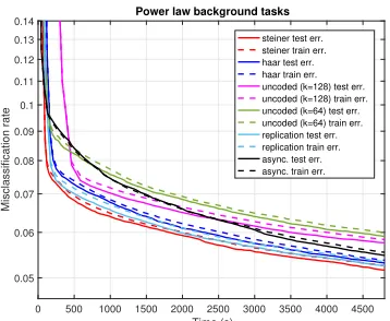
0 500 1000 1500 2000 2500 3000 3500 4000 4500 Time (s)
0.05 0.06 0.07 0.08 0.09 0.1 0.11 0.12 0.13 0.14
Misclassification rate
Power law background tasks
steiner test err. steiner train err. haar test err. haar train err. uncoded (k=128) test err. uncoded (k=128) train err. uncoded (k=64) test err. uncoded (k=64) train err. replication test err. replication train err. async. test err. async. train err.
Figure 13: Test and train errors over time (in seconds) for each scheme. Number of background tasks follow a power law. Steiner and Haar encoding is done with
k= 80,β = 2.
# Nodes (m) Dimensions (n×d) 8 8000×3000 32 32000×12000 128 128000×48000
Table 2: Problem dimensions for each experiment.
communicate using thempi4pypackage. We consider two models for stragglers. In the first model, at each node, we add a random delay drawn from a Gaussian mixture distribution
qN(µ1, σ21) + (1−q)N(µs, σ22), where q = 0.5, µ1 = 0.5s, µs = 20s, σ1 = 0.2s, σ2 = 5s. In the second model, we do not directly add any delay, but at each machine we launch a number of dummy background tasks (matrix multiplication) that are executed throughout the computation. The number of background tasks across the nodes is distributed according to a power law with exponentα= 1.5. The number of background tasks launched is capped at 50.
Figures 12 and 13 shows the evolution of training and test errors as a function of wall clock time. We observe that for each straggler model, either Steiner or Haar encoded optimization dominates all schemes. Figures 14 and 15 show the statistics of how frequent each node participates in an update, for the case with background tasks, for encoded and asynchronous cases, respectively. We observe that the stark difference in the relative speeds of different machines result in vastly different update frequencies for the asynchronous case, which results in updates with large delays, and a corresponding performance loss.
5.3. Speed tests
0 20 40 60 80 100 120 Node id (k)
0 0.1 0.2 0.3 0.4 0.5 0.6 0.7 0.8 0.9 1
P(k
At
)
Figure 14: The fraction of iterations each worker node participates in (the empirical probability of the event{k∈At}), plotted for Steiner encoding with k = 80, m = 128. The number of background tasks are distributed by a power law with α = 1.5 (capped at 50).
0 20 40 60 80 100 120
Node id (k) 0
0.005 0.01 0.015 0.02 0.025
Fraction of updates performed
Figure 15: The fraction of updates per-formed by each node, for asynchronous block coordinate descent. The horizontal line represents the uniformly distributed case. The number of background tasks are distributed by a power law with α = 1.5 (capped at 50).
Scheme Runtime (s) µs= 0 Runtime (s) µs=γ Runtime (s) µs= 2γ Steiner 1.71 2.10 2.13
Synchronous 1.00 7.93 14.89 Replication 1.03 2.11 3.16 Asynchronous 0.61 -
-Table 3: The average wall-clock time taken to achieve 1.05×MMSEfor each scheme, for
m= 8 workers.
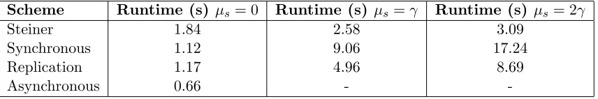
Scheme Runtime (s) µs= 0 Runtime (s) µs=γ Runtime (s) µs= 2γ Steiner 1.84 2.58 3.09
Synchronous 1.12 9.06 17.24 Replication 1.17 4.96 8.69 Asynchronous 0.66 -
-Table 4: The average wall-clock time taken to achieve 1.05×MMSEfor each scheme, for
m= 32 workers.
Scheme Runtime (s) µs= 0 Runtime (s) µs=γ Runtime (s) µs= 2γ Steiner 6.64 15.18 18.51
Synchronous 3.69 43.60 84.55 Replication 4.56 26.55 49.75 Asynchronous 8.77 -
-Table 5: The average wall-clock time taken to achieve 1.05×MMSEfor each scheme, for
straggler mitigation schemes, namely replication and asynchronous optimization, as well as the uncoded synchronous case. To do this, we focus on ridge regression, and use the mean-squared error (MSE) in predicting the test-set response variabley as our metric. We compare the methods against each other by measuring the wall-clock time of optimization required to achieve a fixed mean-squared error.
Note that since the speed-up is due to the mitigation of stragglers, the performance of the proposed technique depends strongly on many cluster- and problem-specific factors, such as computational power of nodes, number of nodes, background processes running at nodes, networking configurations, latency and bandwidth available in the network, compute-to-communication ratio required by the problem, availability of nodes9. Since these experi-ments are intended purely as speed measureexperi-ments, we make several design decisions to build a highly-controlled computing environment, in order to isolate the effects of the straggler mitigation technique and side-step problem- or network-specific artifacts that might affect the results.
First, to have direct control over the delays induced by the workers and measure the exact effect of the delay distribution on the runtime, we use compute-optimized, high-performance, high-bandwidthc4.4xlargeandc4.largeinstances available through Ama-zon EC2, set a node to be a straggler with probabilityq = 0.25, and for stragglers in each step we add an artificial delay drawn from Gaussian distribution N µs, σs2
, to simulate more unreliable clusters. In our tests, we vary µs to measure the effect of the amount of straggler delay (keeping σs = 0.4µs). We sweep µs over the values {0, γ,2γ}, where γ is chosen as the amount of time it takes for a non-straggler node to perform 5-6 iterations for the given problem dimensions. Note that such delays can be observed in practice in un-reliable/burstable clusters (see, for instance, the EC2 experiments in Tandon et al. (2016) conducted ont2.microinstances, where the stragglers are 8×slower, or Ananthanarayanan et al. (2013) which similarly reports 8×straggler delay for latency-limited tasks).
Second, as we scale the number of workers, we scale the problem proportionally as well, in order to maintain the same computation-communication ratio. To be able to control exact problem dimensions, we use synthetic data, where the data matrix X ∈ Rn×d is generated i.i.d. N (0,1), and y=Xw¯+η for some ground truth ¯wand noiseη∈ N 0, ση2, withσ2η proportional ton.
Third, since under data-parallelism the proposed method does not converge to the exact minimum, we first find the minimum MSE (MMSE) achieved for the given problem through a preliminary experiment using fully synchronous optimization with all nodes, as well as hyper-parameter optimization to determine a good value for the regularization parameter
λ, which we determine to beλ= 0.025. Then, we set the MSE bar as 1.05×MMSE. Note that if the exact minimum is desired for encoded scenarios in a real application, one can always increase kt to m (i.e., start using all nodes) towards the end of the optimization, after this approximate target is reached.
Under this setup, we perform three experiments, sweeping the number of workers in the setm∈ {8,32,128}. The problem dimensions for each case is given in Table 2. For encoding we use Steiner ETFs described in Section 4 with redundancy β = 2, and kt = 0.75m. In
all cases, we use gradient descent with step size αt = 0.2, which is run for 120 steps. γ is determined to be 0.2s, 0.3s, and 1.2s for the three problem sizes, respectively.
The results are provided in Tables 3–5, where four methods are compared: Steiner en-coding, uncoded synchronous optimization, uncoded asynchronous optimization, and repli-cation, where each data shard is replicated across two nodes, and the faster copy is used in optimization. Note that Steiner encoding and replication schemes have double the data per worker. The results are averaged over 5 trials.
We observe that when there is no delay (µs = 0), the additional computation overhead of encoding (as well as the perturbation of data) results in relatively high runtime to achieve the desired MSE. We see a similar overhead for replication, although replication enjoys the advantage of having access to raw, uncoded data. However, in the regime where the system is bottlenecked by stragglers (µs =γ and µs = 2γ), the scheme results in significant speed up, ranging from approximately 3×to 7×against the uncoded synchronous; and up to 2× against the replication baseline. Note that replication still gets impacted by straggler nodes if both copies of a shard happen to be delayed. When there are no stragglers, and for modest cluster sizes, asynchronous optimization achieves the best performance. However, since the gradient staleness scales linearly with the cluster size, asynchronous performance falls behind Steiner form= 128 workers even in the absence of stragglers. We also observe that when stragglers are introduced, outdated gradients significantly degrade the asynchronous performance, as the desired MSE bar is not reached at the end of 120 steps. We have run the same experiment for the uncoded case with erasures as well; however, the method failed to achieve the MSE target in all the experiments, including the case with µs = 0. This is because the straggler nodes tend to persist their slow computation throughout optimization. In other words, it is usually approximately the same subset of nodes that provide the updates, effectively removing the data stored in straggler nodes from the optimization. Finally, we note that the runtime for the encoded case also increases in the presence of stragglers (though less severely than the other schemes), due to various implementation overheads such as the interruption of the stragglers for the next iteration. However, we believe that part of this overhead could be mitigated in a more efficient implementation.
We conclude from these experiments that encoding can result in large speed-ups in highly unreliable, low-cost clusters which can induce large delays (such as EC2 t2 instances), or clusters with intermittent node availability (such as EC2 spot instances). It is less suited to reliable clusters with high-capacity, high-bandwidth nodes due to the computational overhead associated with it.
Acknowledgments
Appendix A. Proofs of Theorems 2 and 4
In the proofs, we will ignore the normalization constants on the objective functions for brevity. We will assume the normalization √1
η is absorbed into the encoding matrix SA. Let f(w) = kXw−yk2+λh(w). Let
e
ftA := kSAt(Xwt−y)k
2 +λh(w
t), and feA(w) :=
kSAt(Xw−y)k
2+λh(w), where we setA≡A
t. Letwe
∗
t denote the solution to the effective “instantaneous” problem at iteration t,i.e.,we
∗
t = arg minwfeA(w).
Unless otherwise stated, throughout this appendix, we will also denote
w∗ = arg min w
kXw−yk2+λh(w) ˆ
w= arg min w
kSA(Xw−y)k2+λh(w) unless otherwise noted, where Ais a fixed subset of [m].
A.1. Lemmas
Lemma 10 (Approximation error) If S satisfies (6) (BRIP) for any A ⊆ [m] with
|A| ≥k, for any convex set C,
kXwˆ−yk2 ≤κ2kXw∗−yk2,
where κ= 1+1−, wˆ= arg minw∈CkSA(Xw−y)k2, and w∗ = arg minw∈CkXw−yk2.
Proof Define e= ˆw−w∗ and note that
kXwˆ−yk=kXw∗−y+Xek ≤ kXw∗−yk+kXek
by triangle inequality, which implies
kXwˆ−yk2≤
1 + kXek kXw∗−yk
2
kXw∗−yk2. (14) Note that we have
kSA(Xwˆ−y)k2 ≤ kSA(Xw∗−y)k2
by the definition of ˆw. Expanding the quadratic terms and canceling the common term
y>SA>SAy from both sides, we get
ˆ
w>X>SA>SAXwˆ−2y>SA>SAXwˆ≤w∗>X>SA>SAXw∗−2y>SA>SAXw∗.
Adding −2w∗>X>SA>SAXwˆ+w∗>X>SA>SAXw∗ to both sides,
ˆ
w>X>SA>SAXwˆ−2w∗>X>SA>SAXwˆ+w∗>X>SA>SAXw∗−2y>SA>SAXwˆ ≤2w∗>X>SA>SAXw∗−2y>SA>SAXw∗−2w∗>X>SA>SAXw,ˆ
which can be re-arranged into
![Figure 1: Uncoded distributed optimiza-tion with data parallelism, where X andy are partitioned as X = [Xi]i∈[m] andy = [yi]i∈[m].](https://thumb-us.123doks.com/thumbv2/123dok_us/9771526.1962336/4.612.327.523.86.193/figure-uncoded-distributed-optimiza-data-parallelism-andy-partitioned.webp)