Active Generative Adversarial Network for Image Classification

The Thirty-Third AAAI Conference on Artificial Intelligence (AAAI-19)

Active Generative Adversarial Network for Image Classification

Quan Kong,

Bin Tong,

Martin Klinkigt,

Yuki Watanabe,

Naoto Akira,

Tomokazu Murakami

†_{Hitachi, Ltd. R&D Group, Japan} ‡_{Hitachi America, Ltd. USA}

{quan.kong.xz, bin.tong.hh, martin.klinkigt.ut}@hitachi.com

{naoto.akira.vu, tomokazu.murakami.xr}@hitachi.com [email protected]

Abstract

Sufficient supervised information is crucial for any machine learning models to boost performance. However, labeling data is expensive and sometimes difficult to obtain. Active learning is an approach to acquire annotations for data from a human oracle by selecting informative samples with a high probability to enhance performance. In recent emerging stud-ies, a generative adversarial network (GAN) has been inte-grated with active learning to generate good candidates to be presented to the oracle. In this paper, we propose a novel model that is able to obtain labels for data in a cheaper man-ner without the need to query an oracle. In the model, a novel reward for each sample is devised to measure the degree of

uncertainty, which is obtained from a classifier trained with existing labeled data. This reward is used to guide a condi-tional GAN to generate informative samples with a higher probability for a certain label. With extensive evaluations, we have confirmed the effectiveness of the model, showing that the generated samples are capable of improving the classifi-cation performance in popular image classificlassifi-cation tasks.

Introduction

Machine learning models including traditional ones and new emerging deep neural networks require sufficient supervised information, i.e., class labels, to achieve fair performance. In situations in which labeled data is expensive or difficult to obtain, these models degenerate in performance. Active learning (Settles 2009a) is proposed for handling such a problem. It aims to find the best approach to leverage a lim-ited number of labeled data and to reduce the cost of data an-notation. Active learning selects informative samples from a pool of unlabeled data and obtains their labels by involving a human oracle. In this paper, we investigate the problem of lack of labeled data from a new and different perspec-tive. We propose a model to improve learning performance, which is able to make use of limited labeled data without us-ing any additional unlabeled data nor involvus-ing any human oracle to acquire labels.

As to a classification model, informative samples are those that are able to better contribute to improving classi-fication performance than other samples. For example,

sam-∗

contribute equally to this paper.

Copyright c2019, Association for the Advancement of Artificial Intelligence (www.aaai.org). All rights reserved.

ples close to the hyper-plane are oftenuncertainfor a sup-port vector machine (SVM) based classifier. Therefore, ac-quiring labels of those samples can reduce theuncertainty, thereby reducing classification errors. In the area of active learning, informative samples are selected from a pool of unlabeled data by using criteria, such as degree of uncer-tainty. The labels of the selected samples are obtained by querying a human oracle. Recently, there have been attempts (Zhu and Bento 2017; Huijser and van Gemert 2017) which label informative samples generated from a generative ad-versarial network (GAN) (Goodfellow et al. 2014). In these works, GAN is used to generate samples with the same dis-tribution as the unlabeled dataset. In (Zhu and Bento 2017), latent variables, which are able to generate samples that have small distances to the classification hyper-plane, are selected. These latent variables are used to generate sam-ples that are labeled by involving an oracle. In (Huijser and van Gemert 2017), a GAN is used to generate samples com-pound of two classes and the human oracle has to choose the sample which cannot be clearly assigned to either class. However, the above methods still need to use a pool of unla-beled data and query the human oracle.

two-fold:

1. We propose a model that provides a cheaper way than ac-tive learning to acquire labeled samples. Instead of query-ing the oracle, our model generates labeled samples with a higher probability that are informative to optimize the hyper-plane of a classifier.

2. We propose a novel loss function for training generative network model to generate informative samples with a specific label that is inspired by the idea of policy gra-dient (Sutton et al. 2000) in reinforcement learning. We regard generated samples and the external signal related touncertaintyasactionandreward, and use this reward to update the parameters of network for generating infor-mative samples.

Related Work

Relying only a limited amount of labeled data is a long-standing and important problem in the area of machine learning. Different philosophies and problem settings ex-ist for dealing with this, such as transfer learning (Pan and Yang 2010), semi-supervised learning (Rosenberg, Hebert, and Schneiderman 2005) and active learning (Settles 2009a). Transfer learning focuses on how to optimize a model with a limited amount of labeled data by transferring the knowledge from a similar yet different source task with suf-ficient labeled data, thereby reducing the cost of data an-notation for the task at hand. Zero-shot learning (Lampert, Nickisch, and Harmeling 2009; Frome et al. 2013) is a vari-ation of transfer learning, in which unseen, and therefore unlabeled objects are expected to be recognized by trans-ferring knowledge fromseenclasses (Settles 2009a). Semi-supervised learning leverages the unlabeled data to boost the performance in case of only labeled data is used. Ac-tive learning (Settles 2009a) is based on a different philos-ophy. Typically, unlabeled data is available to this learn-ing paradigm, in which the most informative samples from the pool of unlabeled data are selected to query an ora-cle. Active learning provides a schema to limit the num-ber of queries by selecting the most informative samples to maximize the effect of the acquired labels. To deter-mine the degree of uncertainty used in the query strat-egy, uncertainty sampling (Jain and Kapoor 2009) is the most simple, yet widely used criterion to measure informa-tiveness. Other criteria for the query strategy may include query by committee (QBC) (Freund et al. 1997), expected error reduction (Roy and Mccallum 2001; Moskovitch et al. 2007) and density weighted methods (Shen et al. 2004; Donmez, Carbonell, and Bennett 2007; Cebron and Berthold 2009).

A generative adversarial network (GAN) (Goodfellow et al. 2014) is a neural network model trained in an un-supervised manner, aiming to generate new data with the same distribution as the data of interest. It is widely applied in computer vision and natural language processing tasks, such as generating samples of images (Denton et al. 2015) and generating sequential words (Romera-Paredes and Torr 2015). One of its variants, conditional GAN (Mirza and Osindero 2014), uses both label information and noisy latent

variables to generate samples for a specified label. A variant of conditional GAN, called Auxiliary Classifier GAN (AC-GAN) (Odena, Olah, and Shlens 2017), uses supervised in-formation to generate high quality images at pixel level.

Recently, the GAN models have been used with transfer learning (Choe et al. 2017; Bousmalis et al. 2017), zero-shot learning (Tong et al. 2018; Wang et al. 2018), semi-supervised learning (Dai et al. 2017; Lee et al. 2018) and ac-tive learning (Zhu and Bento 2017; Huijser and van Gemert 2017). In (Dai et al. 2017) and (Lee et al. 2018), GAN models are used to train feed-forward classifiers with an additional penalty derived from out-of-distribution samples or low-density samples. It should also be emphasized that both low-density and out-of-distribution samples does not necessarily represent hard samples. For example, out-of-distribution samples, which are far from the classification boundary, will not be regarded as hard samples. Another dif-ference from them lies in that our work focuses on training the generator with an informativeness reward given by the existing classifier. Unlike the works (Zhu and Bento 2017; Huijser and van Gemert 2017) in which the generated sam-ples are presented to the oracle, this work focuses on di-rectly generating informative labeled samples that might contribute to boosting learning performance. To the best of our knowledge, this is the first study that uses a GAN to gen-erate informative samples by incorporating a new devised factor to measure the degree ofuncertainty. This study pro-vides a new paradigm that augments labeled data to improve learning performance without using any other unlabeled data nor involving a human oracle.

Preliminary

In this section, we introduce the preliminaries of GAN and active learning that serves as the basis to derive our new model. A GAN (Goodfellow et al. 2014) consists of a gen-erator Gand discriminatorD that compete in a turn-wise min-max game. The discriminator attempts to distinguish real samples from synthetic samples, and the generator at-tempts to fool the discriminator by generating synthetic sam-ples looking like real samsam-ples. TheDandGplay the follow-ing game onV(D, G)

min

G maxD V(D, G) =Exi∈pdata(x)[logD(xi)] +

Ez∈pz(z)[log(1−D(G(z)))], (1) where xi represents a sample.pdata and pz represent the distribution of real samples and synthetic samples, and z

represents a noise vector. A GAN tries to mappz topdata; that means the generated samples fromGare desired to own a high likeness withpdatawhich is also the distribution of training samples. In the original GAN model onlyzis used to generate samples. In a variation called conditional GAN (CGAN) (Mirza and Osindero 2014), a conditionyi, which is a class label ofxi, is included in addition tozto control the sample generation. The objective function becomes

min

G maxD V(D, G) =Exi∈pdata(x)[logD(xi|yi)] +

𝒛~𝒑𝒛

class label

𝒚𝒊

𝐼′

𝐼

Classifier𝑪 Generator

Discriminator

smallest margin label entropy

Reward Synthetic

Sample Real Sample

𝑃_𝑦𝑖0

𝑃_𝑦

𝑖1

⋮ 𝑃𝑦𝑖𝑛

class probability

Classification Loss

real/fake Adversarial Loss

Linear Layer Conv Layer

Likelihood

Gaussian MLP

Uncertainty Loss

ReLU Layer

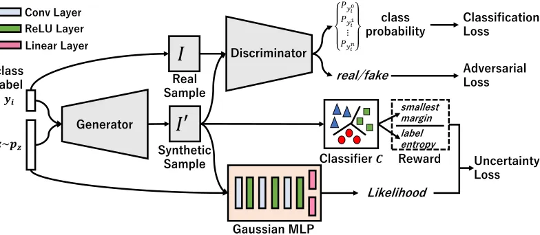
Figure 1: Architecture of our proposed model.I.The generator generates samples by training a generator and a discriminator with a class label one hot vectoryifrom training sample as a condition. In our case, we introduce a Classification Loss follows AC-GAN (Odena, Olah, and Shlens 2017) to make sure the generated sample is highly related to the specific given label condition. The discriminator also determines the possibility if a generated sample is fake, which is used as our Adversarial Loss to make the distributions of generated and real samples similar.II.Simultaneously, a classifierCtrained with existing labeled data. It calculates a reward for a sample related to the degree ofuncertaintyincludes the smallest margin and label entropy.III. A Gaussian Multi-Layer Perceptron (MLP) (Duan et al. 2016) calculates a likelihood of a sample to be generated from current distribution of synthetic samples. Uncertainly Loss consists of a likelihood and rewards of each generated sample, and we use it to train the generator for generating informative samples via policy gradient.

whereyicould be a one-hot representation of the class label. During training of the CGAN model,yi is used to instruct the generatorGto synthesize samples for this given class.

Active learning is a machine learning method that is able to interactively query an oracle to obtain labels for samples. These samples are selected from an unlabeled sample pool by using a criterion to measure if the selected sample is able to reduce the learning error. To be more specific, standard supervised learning problems assume an instance space of dataX and labels Y. A mapping functionf : X → Y is optimized by minimizing error:

f∗= arg min f∈F

X

Y

L(f(X), Y), (3)

whereFrepresents a space over a predefined class of func-tions. The error is measured by a loss functionL that pe-nalizes disagreement betweenf(X)andY. In the typical setting of active learning (Settles 2009b), a pool of unla-beled samplesU = {xu

1, . . . ,xun} is given. Denote M =

{(x1, y1), . . . ,(xn, yn)}, wherexi ∈Xandyi∈Y. Active learning performs in an iterative way: (1) training a classifier

f onM; (2) using a query functionQ(f, M, U)to select an unlabeled samplei∗to label; (3) removingxu

i∗ fromU and

adding(xu

i∗, yi∗)toM. The target of active learning is to

choose samples i∗ to be labeled by asking an oracle, and reduce the learning error with as few queries as possible. The selected samples are regarded as more informative than other unselected ones in terms of contribution in learning error reduction.

Proposed Method

In this section, we discuss the details of the proposed method. Without loss of generality, we take a classifier as the example of supervised learning, in which we are given a set of labeled dataSl ={(x1, y1),(x2, y2), . . . ,(xN, yN)} wherexi is a sample,yi is its corresponding label, andN represents the number of samples.

The overview of our proposed model is shown in Figure 1. This model mainly consists of a classifierCtrained with existing labeled data, a conditional GAN, and a Gaussian Multi-Layer Perceptron (MLP) (Duan et al. 2016). The con-ditional GAN is used to generate labeled samples. A novel reward is devised to measure the degree of informativeness for each generated sample. This reward is calculated accord-ing to a degree ofuncertaintyfor a sample with respect to the hyper-plane of the pre-trained classifier. In general, the more informative a sample is, the higher probability this sample is able to improve classification performance if it is included in the existing labeled data. The Gaussian MLP provides a likelihood of a generated sample to be generated from a re-cent set of generated samples. Together with the likelihood, the reward is used to update parameters for the generator in the conditional GAN. This model makes a trade-off between generating samples with the same distribution as the labeled data and generating informative samples to improve classi-fication performance for the pre-trained classifier.

Generation of labeled samples

performance on generating images.

Given a set of labeled images{(x1, y1), . . . ,(xN, yN)}, the AC-GAN model is used to generate labeled samples with the inputs of both a noise latent variable and a one-hot rep-resentation of a class label. In the AC-GAN, the generatorG

generates a synthetic sample_bxi = G(z, yi)with the noise latent vectorz and a labelyi. The discriminator gives two kinds of probabilities. One is a probability distribution over sources, i.e., P(real|xi) andP(fake|_bxi). The other one is posterior probabilities over the class labels, i.e., P(yi|xi) andP(yi|_bxi). The objective functions of generator and dis-criminator in the AC-GAN are formulated as

LD_AC-GAN =E[logP(real|xi)] +E[logP(fake|xbi)]+

E[logP(yi|xi)] +E[logP(yi|bxi)]

(4)

LG_AC-GAN =_E[logP(real|x_bi)] +E[logP(yi|xbi)]. (5)

The discriminator D is trained to maximize LD

AC-GAN, and

the generatorGis trained to maximizeLG

AC-GAN. For the

dis-criminator D, the first two terms in Equation 4 encourage that both real and fake samples are classified correctly. The last two terms in Equation 4 encourage that both real and fake samples have correct class labels. For the generatorG, it is expected that generated samples are classified as fake, and have correct class labels as well.

Measure of uncertainty

In this subsection, we discuss how the degree ofuncertainty is measured in the proposed model. Among the samples gen-erated by the AC-GAN model, only informative samples might be able to contribute to improving classification per-formance. In the area of active learning, uncertainty sam-pling is the most widely used query strategy. The intuition behind uncertainty sampling is that if a sample is highly un-certain with a hyper-plane of a classifier, obtaining its label will improve the degree of discrimination among classes. In other words, this sample is considered to be informative in improving the classification performance. In our model, we use SVM as the classifier. In our paper, we mainly use two metrics based on the label probabilities to measure the un-certainty of a sample.

Smallest MarginMargin sampling is an uncertainty sam-pling method in the case of multi-class (Settles 2009a), which is defined as

b

xM = arg min

b

xi

(P(y₁0|x_bi)−P(y20|bxi)), (6)

wherey₁0 andy0₂are the first and second most probable class labels of a generated sample_bxi under the specified classi-fier, respectively. Intuitively, samples with large margins are easy, since the classifier has little doubt in differentiating be-tween the two most likely class labels. Samples with small margins are more ambiguous, thus knowing the true label will help the model to discriminate more effectively between them.

Label Entropy A more general uncertainty sampling strategy uses the entropy of posterior probabilities over class labels. In smallest margin, posterior probabilities of labels

other than the two most probable class labels are simply ig-nored. To mitigate this problem, the entropy over all class labels is used, which is formulated as

b

xLE= arg max

b

xi

−X

y0

p(y0|_bxi) logp(y0|x_bi). (7)

Loss on uncertainty

In this subsection, we discuss how to devise a loss function for the generated samples based on the degree ofuncertainty to update the parameters of the generator.

Policy gradient (Sutton et al. 2000) has been successfully applied in reinforcement learning to learn an optimal pol-icy. As one target of this work is to guide the generator to synthesize informative samples, we regard the degree of un-certainty and the generated samples asrewardandaction, respectively. In general, the higher the degree ofuncertainty is, the higher the reward is obtained. If a generated sample has a high degree ofuncertainty, this sample is encouraged to be generated with a high probability. To the best of our knowledge, we are the first to use the idea from policy gra-dient to model the degree ofuncertaintyin active learning.

In the following we discuss how to convert the degree ofuncertaintyinto a reward. With respect to smallest mar-gin, for each generated sample_bxi, the reward can be simply calculated byrm(bxi) = e

−um_{, whereu}

m = P(y10|bxi)− P(y₂0|_bxi). If the difference between the probabilities of the two most probable class labels for a generated sample is small, this generated sample is uncertain. This results in a larger value ofrmthan other certain samples. Based on the nature of Equation 6, umfalls into the range of[0,1]. The values ofrm, which fall in the range[1_e,1], have no signifi-cant difference between the best and worst cases, which may result in an inappropriate design of the reward. Inspired by (Lee et al. 2018), we set a thresholdto truncate the value of reward for a bad case where the margin of two probabilities is large. Specifically, given a threshold, the reward is

rm(bxi) =

e−um_{, ifu}

m≤

C, otherwise (8)

whereCis a constant number. In our work, we set its value to0, which means that ifumis larger than, we enforce the rewardrmto be zero.

With respect to label entropy, we can calculate the reward similar to rle(x_bi) = eule, where ule =

−P

y0p(y0|x_bi) logp(y0|bxi). The reward for a generated sample is calculated by combining the above two factors, which is formulated as

r(_bxi) =α·rm(x_bi) + (1−α)·rle(x_bi), (9)

whereαis a parameter that balances the importance between the two metrics of smallest margin and label entropy. Ac-cording to policy gradient, we devise the loss for generated samples formulated as follows:

Luncertainty=

X

b

xi

r(x_bi)P(xbi|θ), (10)

generated by the generator. However, the generator does not directly provide such a probability for each generated sam-ple. Therefore, we have to estimate this probability based on a model with the parameters θ. In our work, we choose a MLP to parameterize the policy. We use a Gaussian distri-bution over action space, where the covariance matrix was diagonal and independent of the state. The Gaussian MLP maps from the input synthetic imageG(z, yi)to the mean µand standard deviationσof a Gaussian distribution with the same dimension asz. Thus, the policy is defined by the normal distributionN(θ|µ, eσ_{). Then we can compute the} likelihood P(G(z, yi)|θ)withµandσ from the output of approximated Gaussian MLP. The Gaussian MLP is jointly learned withGandDby policy gradient.

Algorithm 1ActiveGAN

Input training data xi and its label yi where i ∈ [1, . . . , N].

OutputΨd(parameters of D),Ψg(parameters of G) and θ(parameters of MLP)

1: Initializeα,λ,θ,ΨdandΨg.

2: Set the buffer size to beM

3: Train SVM with grid-search for best parameters

4: Train the generatorGand the discriminatorDwith first

miterations

5: Save generated samples inmiterations into the buffer

6: repeat

7: Generate a samplex_bi←G(z, yi)

8: Use Equation 9 to calculate the rewardr(_bxi)forbxi.

9: Use generated samples to calculate the likelihood

P(_bxi|θ)forxbi

10: Use Equation 10 to calculate the loss LU related to the degree ofuncertaintyfor_bxi

11: Update parameters for the generator Gand M LP: Ψg,θ←(Ψg,θ) +5Ψg,θL

G

ActiveGAN(Ψg, θ)

12: Update parameters for the discriminatorD:Ψd←Ψd +5ΨdL

D

AC-GAN

13: Update the buffer by adding the sample_bxi

14: until

Algorithm

By integrating the loss measuring the degree ofuncertainty for the generated samples, our proposed model, called Ac-tiveGAN, has the following loss function for the generator, which is maximized.

LG_ActiveGAN=LG_AC-GAN+λLuncertainty

=_E[logP(real|_bxi)] +E[logP(y|bxi)]

+λE[P(xbi|θ)r(bxi)], (11)

whereLG

AC-GAN is the loss function of the generator in

AC-GAN. The discriminator in Active-GAN is the same as that in AC-GAN, which is denoted byLD

ActiveGAN. The notations

ΨgandΨdin Algorithm 1 represent the parameters of gen-erator and discriminator in the ActiveGAN, respectively.λ

is a parameter that balances the importance between the loss for the generator in the AC-GAN model and the loss related

to the degree ofuncertaintyfor the generated samples. The larger the value ofλis, the more likely the model is forced to generate samples that contribute to improving the classi-fication performance instead of generating samples whose distribution is the same as the training ones. The learning process of ActiveGAN is depicted in detail in Algorithm 1. Following (Sutton et al. 2000), the gradient of the objective functionLuncertaintycan be derived as

5Ψg,θLuncertainty=E[5Ψg,θlogP(GΨg(z, yi)|θ)r(xbi)] (12)

The evaluation of ActiveGAN is conducted as follows. We use the trained generatorGto synthesize a specific num-ber of samples, which we denoted bySg. Together with the labeled dataSl, we retrain the SVM to examine if improve-ment of classification performance is achieved.

Experiments

In this section, we introduce evaluation settings and discuss performances of models. We then make analysis for a further understanding on our model.

Evaluation settings

We utilized four datasets CIFAR10 (Krizhevsky, Nair, and Hinton ), MNIST (Netzer et al. 2011), Fashion-MNIST (Xiao, Rasul, and Vollgraf 2017) and a large scale dataset Tiny-ImageNet (Russakovsky et al. 2015) for evaluation of the proposed model ActiveGAN. MNIST consists of 50,000 training samples, 10,000 validation samples and 10,000 test-ing samples of handwritten digits of size 28×28. CIFAR10 has colored images for 10 general classes. Again we find 50,000 training samples and 10,000 testing samples of size 32×32 in CIFAR10. Fashion-MNIST has a training set of 60,000 examples and a test set of 10,000 examples. Each example is a 28×28 grayscale image, associated with a la-bel from 10 different classes associated with fashion items. Tiny-ImageNet has 200 classes, each class has 500 training images, 50 validation images, and 50 test images. All images are 64×64.

We used the same network structure for the generator and discriminator as in (Odena, Olah, and Shlens 2017) for CIFAR-10 and (Chen et al. 2016) for MNIST and Fashion-MNIST. We downsized Tiny-ImageNet samples from 64

× 64 to 32 × 32 and use the same network structure as CIFAR-10. To train a stable ActiveGAN, the parameters of the discriminator are updated once after those of the gener-ator are updated for a specified number of iterations. Adam was used as the gradient method for learning parameters of the network. Its initial learning rate is searched in the set

{0.0002,0.001}. We used SVM as a base classifier and its optimal hyper-parameters are chosen via a grid search. We used a pre-trained VGG-16 (Simonyan and Zisserman 2014) to extract features for images for all datasets. The threshold

in Equation 8 was set to0.2. The balancing parameterα

in Equation 9 was set to0.5. The balancing parameterλin Equation 11 was set to0.1to guarantee that values of two termsLG_AC-GANandLUare in the same scale.

Table 1: F-score of models on CIFAR-10, MNIST, Fashion-MNIST (F-MNIST) and Tiny-ImageNet.nrepresents the number of labeled images used for training.

CIFAR-10 MNIST F-MNIST Tiny-ImageNet

Method n=5k n=10k n=500 n=1k n=5k n=10k n=10k n=20k

Baseline(SVM) 83.4 85.3 94.6 96.2 87.1 88.1 56.1 58.3

AC-GAN 81.4 82.7 94.1 95.8 85.4 86.4 52.2 56.1

AC-GAN+F 82.5 83.2 94.5 95.9 86.2 87.3 53.2 56.9

ActiveGAN 84.3 86.3 95.1 96.5 87.6 89.0 57.5 59.4

set, the generated images from AC-GAN or ActiveGAN are used to retrain the SVM. For the fair comparison, we had two different settings for dealing with those generated im-ages for the compared method AC-GAN. The first setting is to use all generated images from AC-GAN. The second one is to use the model, denoted by AC-GAN+F, in which sam-ples are generated from AC-GAN and an additional filter with a margin is then applied to these generated samples to obtain informative samples. This filter attempts to filter out the samples that overlap the training samples, leaving sam-ples outside the distribution of training samsam-ples. The margin

um, which is the difference of posterior probabilities of the two most probable class labels, is calculated by Equation 6 and this margin was tuned in our evaluation. The F-score is used as the metric for evaluating performance. F-score is calculated by2_P·P₊·_RR, wherePareRare precision and recall, respectively.

Image Classification

Table 1 shows the classification performances of mod-els for four different datasets. Note that the margin for AC-GAN+F was also tuned for each data set in the set

{0.1,0.15,0.20,0.25,0.3}. The best F-scores were chosen, which are 0.2, 0.15, 0.15, and 0.2 in CIFAR-10, MNIST, F-MNIST and Tiny-ImageNet, respectively. We chose the number of training samplesnas500or 1,000for MNIST and as5,000or10,000for the other datasets. Note that all test samples in each dataset were used.

We can see that when the number of images used for train-ing the baseline SVM increases, F-scores were improved in every dataset. When the generated images from AC-GAN were used for training together with the existing labeled im-ages, the classification performance even dropped. For in-stance, in the dataset CIFAR-10, the classification perfor-mance dropped by2.0points and2.5points in the cases of

n set to 5,000 and10,000, respectively. By applying the additional filter with the smallest margin, the classification performances of AC-GAN+F were slightly improved. How-ever, the side effect is not fully mitigated, and performances were still lower than the baseline SVM. This empirically ex-plains that the generated samples from AC-GAN, whose dis-tribution was similar to that of images in the original training data, did not provide more information than what the origi-nal training images provide.

Using the generated samples from ActiveGAN is able to achieve better performance than the baseline classifier for all dataset without any additional data. For instance, for

the dataset CIFAR10, ActiveGAN is able to achieve bet-ter performance than the baseline SVM by 0.9points and 1.0 points. For the more complex dataset Tiny-ImageNet, ActiveGAN achieved F-scores of57.5and59.4in two dif-ferent settings, which are improvements of 1.4 points and 1.1 points compared to the baseline SVM, respectively. These results confirm the superiority of our model over the baselines in both small-scale and large-scale image classifi-cation, which may bring ActiveGAN into a practical use.

D: cat

J: truck

E: deer

H: horse

C: bird

F: dog

I: ship

G: frog

A: airplane

B: automobile

-0.5 0 0.5 1 1.5 2 2.5 3 3.5 4 Improvements of F-score per class

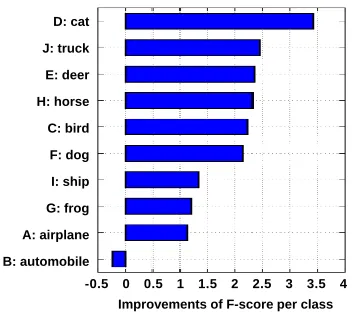
Figure 2: F-score improvements of each class compared with baseline SVM in the dataset CIFAR-10. The number of im-ages used in the training is10k.

For an in-depth analysis, we also showed how the F-scores of each category changes compared to the baseline SVM if ActiveGAN is used. Figure 2 shows improvements of F-score for each class in the dataset CIFAR-10. We can observe that, except the class ‘automobile’, F-scores of the other classes were improved. Among the improvements, the F-score of the class ‘cat’ was improved by3.42points.

Discussion and Analysis

We examined the impact of hyper-parameterin Equation 8 by using CIFAR10 data. The result is shown in Table 2. Note that the value ofrm(_bxi)without a truncation of the thresholdfalls into the range[1

when is set to 0.2. Setting to1.0 is an extreme case. It means that the reward from smallest margin is degraded to rm(bxi) = e

−um_{. Its performance is the worst among} the other settings of. It is because the generated samples, which are certain to the classifier, receive little penalty.

Table 2: F-scores whenchanges forn=10k.

0.0 0.1 0.2 0.3 0.4 0.5 0.6 1.0

F-score 85.4 85.7 86.3 85.8 85.3 85.2 85.1 85.0

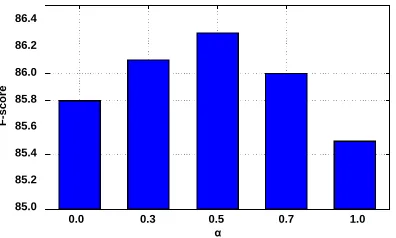
In order to verify the effectiveness of reward derived from both smallest margin and label entropy in generating infor-mative samples, we showed the impact ofαin Equation 9 by using CIFAR-10 data. The result is shown in Figure 3. We can see that when α is set to 0.0, only label entropy is used for calculating the reward. Its performance outper-formed about 2.6 points compared with AC-GAN+F. When we only use smallest margin as the reward (α = 1.0), the performance was boosted by 2.3 points. Whenαwas set to 0.5, the best performance was achieved, which is 0.5 and 0.8 points higher than those whenαwas set to0.0and1.0, respectively. This implies that both criterion of smallest mar-gin and label entropy are helpful for generating informative samples.

86.4

86.2

86.0

85.8

85.6

85.4

85.2

85.0

α

F

-score

0.0 0.3 0.5 0.7 1.0

Figure 3: F-scores whenαchanges for n=10k.

(a) AC-GAN (b) ActiveGAN

Figure 4: This is t-SNE visualization of the generated sam-ples from AC-GAN (a) and ActivGAN (b) on CIFAR-10, which are denoted by green points. The red points are the real hard samples selected from test data pool by using smallest margin, which is calculated by Equation 6. For a fair comparison, we set the smallest margin to0.2, which is the same as= 0.2 used in ActiveGAN. The light blue points denote training samples randomly sampled from each class.

Figure 5: Samples of generated images from ActiveGAN in the dataset CIFAR-10. Each column shares the same label and each row shares the same latent variables.

To verify that ActiveGAN is more likely to generate infor-mative images than AC-GAN, we visualized the features of training images and the generated images in CIFAR10 in a2 -dimensional space, as shown in Figure 4. The2-dimensional space is obtained by t-distributed stochastic neighbor em-bedding (t-SNE). As shown in Figure 4a, the generated sam-ples of AC-GAN highly overlap the training samsam-ples dis-tribution. As shown in Figure 4b, by using our loss about uncertainty, the generated samples of ActiveGAN tends to distribute outside of the training samples. It can be also seen that some generated samples from ActiveGAN fall in the area of real hard samples, which is very unlike AC-GAN.

We showed the sampled images from original training im-ages and ActiveGAN on CIFAR-10, as depicted in Figure 5. The first column of Figure 5 represents images of class la-bel ‘airplane’. We can see that some images in Figure 5 look like ‘bird’, which might serve as informative images to dis-criminate the classes of ‘airplane’ and ‘bird’.

Conclusion

In this paper, we investigate the problem of lack of la-beled data, in which labels of data can be obtained with-out using any additional unlabeled data nor querying the human oracle. In this work, we use class-conditional gen-erative adversarial networks (GANs) to generate images, and devise a novel reward related to the degree of uncer-taintyfor generated samples. This reward is used to guide the class-conditional GAN to generate informative samples with a higher probability. Our empirical results on CIFAR10, MNIST, Fashion-MNIST and Tiny-ImageNet demonstrate that our proposed model is able to generate informative la-beled images that are confirmed to be effective in improving classification performance.

References

adap-tation with generative adversarial networks. InCVPR, 95– 104.

Cebron, N., and Berthold, M. R. 2009. Active learning for object classification: from exploration to exploitation. Data Mining and Knowledge Discovery18(2):283–299.

Chen, X.; Chen, X.; Duan, Y.; Houthooft, R.; Schulman, J.; Sutskever, I.; and Abbeel, P. 2016. Infogan: Interpretable representation learning by information maximizing genera-tive adversarial nets. InNIPS. 2172–2180.

Choe, J.; Park, S.; Kim, K.; Park, J. H.; Kim, D.; and Shim, H. 2017. Face generation for low-shot learning using gen-erative adversarial networks. InWorkshop of ICCV. Dai, Z.; Yang, Z.; Yang, F.; Cohen, W. W.; and Salakhutdi-nov, R. 2017. Good semi-supervised learning that requires a bad gan. InNIPS, 6513–6523.

Denton, E.; Chintala, S.; Szlam, A.; and Fergus, R. 2015. Deep generative image models using a laplacian pyramid of adversarial networks. InNIPS, 1486–1494.

Donmez, P.; Carbonell, J. G.; and Bennett, P. N. 2007. Dual strategy active learning. In Kok, J. N.; Koronacki, J.; Man-taras, R. L. d.; Matwin, S.; Mladeniˇc, D.; and Skowron, A., eds.,ECML, 116–127.

Duan, Y.; Chen, X.; Houthooft, R.; Schulman, J.; and Abbeel, P. 2016. Benchmarking deep reinforcement learn-ing for continuous control. InICML, 1329–1338.

Freund, Y.; Seung, H. S.; Shamir, E.; and Tishby, N. 1997. Selective sampling using the query by committee algorithm. Machine Learning28(2):133–168.

Frome, A.; Corrado, G. S.; Shlens, J.; Bengio, S.; Dean, J.; Ranzato, M. A.; and Mikolov, T. 2013. Devise: A deep visual-semantic embedding model. InNIPS, 2121–2129. Goodfellow, I. J.; Pouget-Abadie, J.; Mirza, M.; Xu, B.; Warde-Farley, D.; Ozair, S.; Courville, A. C.; and Bengio, Y. 2014. Generative adversarial nets. InNIPS, 2672–2680. Huijser, M. W., and van Gemert, J. C. 2017. Active decision boundary annotation with deep generative models. InICCV, 5296–5305.

Jain, P., and Kapoor, A. 2009. Active learning for large multi-class problems. InCVPR, 762–769.

Krizhevsky, A.; Nair, V.; and Hinton, G. Cifar-10.

Lampert, C. H.; Nickisch, H.; and Harmeling, S. 2009. Learning to detect unseen object classes by between-class attribute transfer. InCVPR, 951–958.

Lee, K.; Lee, H.; Lee, K.; and Shin, J. 2018. Train-ing confidence-calibrated classifiers for detectTrain-ing out-of-distribution samples. InICLR.

Mirza, M., and Osindero, S. 2014. Conditional generative adversarial nets.CoRRabs/1411.1784.

Moskovitch, R.; Nissim, N.; Stopel, D.; Feher, C.; Englert, R.; and Elovici, Y. 2007. Improving the detection of un-known computer worms activity using active learning. In Advances in Artificial Intelligence, 489–493.

Netzer, Y.; Wang, T.; Coates, A.; Bissacco, A.; Wu, B.; and Ng, A. Y. 2011. Reading digits in natural images with

unsupervised feature learning. InNIPS Workshop on Deep Learning and Unsupervised Feature Learning.

Odena, A.; Olah, C.; and Shlens, J. 2017. Conditional im-age synthesis with auxiliary classifier gans. InICML, 2642– 2651.

Pan, S., and Yang, Q. 2010. A Survey on Transfer Learning. IEEE TKDE22(10):1345–1359.

Romera-Paredes, B., and Torr, P. H. S. 2015. An embar-rassingly simple approach to zero-shot learning. InICML, 2152–2161.

Rosenberg, C.; Hebert, M.; and Schneiderman, H. 2005. Semi-supervised self-training of object detection models. In WACV/MOTION, volume 1, 29–36.

Roy, N., and Mccallum, A. 2001. Toward optimal active learning through sampling estimation of error reduction. In ICML, 441–448.

Russakovsky, O.; Deng, J.; Su, H.; Krause, J.; Satheesh, S.; Ma, S.; Huang, Z.; Karpathy, A.; Khosla, A.; Bernstein, M.; Berg, A. C.; and Fei-Fei, L. 2015. Imagenet large scale visual recognition challenge. IJCV115(3):211–252. Settles, B. 2009a. Active learning literature survey. Computer Sciences Technical Report 1648, University of Wisconsin–Madison.

Settles, B. 2009b. Active learning literature survey. Computer Sciences Technical Report 1648, University of Wisconsin–Madison.

Shen, D.; Zhang, J.; Su, J.; Zhou, G.; and Tan, C.-L. 2004. Multi-criteria-based active learning for named entity recog-nition. InACL, 589–596.

Simonyan, K., and Zisserman, A. 2014. Very deep convo-lutional networks for large-scale image recognition. CoRR abs/1409.1556.

Sutton, R. S.; McAllester, D. A.; Singh, S. P.; and Mansour, Y. 2000. Policy gradient methods for reinforcement learning with function approximation. InNIPS. 1057–1063. Tong, B.; Klinkigt, M.; Chen, J.; Cui, X.; Kong, Q.; Mu-rakami, T.; and Kobayashi, Y. 2018. Adversarial zero-shot learning with semantic augmentation. InAAAI, 2476–2483. Wang, W.; Pu, Y.; Verma, V. K.; Fan, K.; Zhang, Y.; Chen, C.; Rai, P.; and Carin, L. 2018. Zero-shot learning via class-conditioned deep generative models. InAAAI, 4211–4218. Xiao, H.; Rasul, K.; and Vollgraf, R. 2017. Fashion-mnist: a novel image dataset for benchmarking machine learning algorithms.