Stock Prediction using ARMA

(1)

19 Copyright © 2018. IJEMR. All Rights Reserved.

Volume-8, Issue-2, April 2018

International Journal of Engineering and Management Research

Page Number: 19-35

DOI:

doi.org/10.31033/ijemr.v8i02.11607

An in Depth Review Paper on Numerous Image Mosaicing Approaches

and Techniques

Mohamed Abdul – Rahim. M.I.1 and Zheng – Sheng Yu2

1_{MS.c Student, Department of Computer Science, Hang Zhou Dianzi University, CHINA} 2_{Professor, Department of Computer Science and Technology, Hang Zhou Dianzi University, CHINA}

2_{Corresponding Author: [email protected]}

ABSTRACT

Image mosaicing is one of the most important subjects of research in computer vision at current. Image mocaicing requires the integration of direct techniques and feature based techniques. Direct techniques are found to be very useful for mosaicing large overlapping regions, small translations and rotations while feature based techniques are useful for small overlapping regions. Feature based image mosaicing is a combination of corner detection, corner matching, motion parameters estimation and image stitching.

Furthermore, image mosaicing is considered the process of obtaining a wider field-of-view of a scene from a sequence of partial views, which has been an attractive research area because of its wide range of applications, including motion detection, resolution enhancement, monitoring global land usage, and medical imaging. Numerous algorithms for image mosaicing have been proposed over the last two decades.

In this paper the authors present a review on different approaches for image mosaicing and the literature over the past few years in the field of image masaicing methodologies. The authors take an overview on the various methods for image mosaicing.

This review paper also provides an in depth survey of the existing image mosaicing algorithms by classifying them into several groups. For each group, the fundamental concepts are first clearly explained. Finally this paper also reviews and discusses the strength and weaknesses of all the mosaicing groups.

Keywords-- Image mosaicing, Registration, Blending, Geometric Transformation, Homography, Low-level Feature, Transition smoothening, Optimal Seam, Extraction

I. INTRODUCTION

Nowadays, image mosaicing is gaining a lot of interests in the research community for both its scientific significance and potential derivatives in real world applications. Image mosaicing technology is becoming more and more popular in the fields of image processing,

computer graphics, computer vision and multimedia. It is widely used in daily life by stitching pictures into panoramas or a large picture which can display the whole scenes vividly. Given for example, it can be used in virtual travel on the internet, building virtual environments in games and processing personal pictures. Image mosaicing is firstly divided into rectangular sections which are usually equal sized, each of which is replaced with another photograph that matches the target photo. When viewed at low magnifications, the individual pixels appear as the primary image, while close examination reveals that the image is in fact made up of many hundreds or thousands of smaller images.

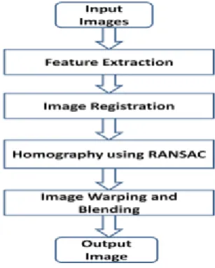
In image mosaicing two input images are taken and these images are fused to form a single large image. This merged single image is the output mosaiced image.

The first step in Image mosaicing is feature extraction. In feature extraction, features are detected in both input images. Image registration refers to the geometric alignment of a set of images. The different sets of data may consist of two or more digital images taken of a single scene from different sensors at different time or from different points of view. In image registration the geometric correspondence between the images is established so that they may be transformed, compared and analysed in a common reference frame.

According to [11] registration methods can be loosely divided into the following classes: algorithms that use image pixel values directly for example; correlation methods; algorithms that use the frequency domain, for example, Fast Fourier transform based (FFT-based) methods [7]; algorithms that use low level features such as edges and corners, for example, Feature based methods [39]; and algorithms that use high-level features such as identified parts of image objects, relations between image features, for example, Graph-theoretic methods [39].

(2)

20 Copyright © 2018. IJEMR. All Rights Reserved.

registration transformations to get the output mosaiced image. The two elements given most importance in image mosaicing are the quality of the mosaicked image and the time efficiency of the algorithm used.

The goal of the stitching step is to overlay the aligned images on a larger canvas by merging pixel values of the overlapping portions and retaining pixels where no overlap occurs. Errors propagated through geometric and photometric misalignments often result in undesirable object discontinuities and seam visibility in the vicinity of the boundary between two images. Thus, a blending algorithm needs to be used during or after the stitching step in order to minimize the discontinuities in the global appearance of the mosaic.

The previously mentioned registration step has been conceived to work with images with a single color band. Different techniques have been used by different mosaicing algorithms to deal with multiple color bands. Given for example, in [60] [3] [55] [1] one of the color bands of the input RGB images are taken into consideration while obtaining the transformation parameters. On the other hand in [21] [37] [61] the RGB images are first converted to grayscale and then transformation parameters are obtained. In either case, after finding the optimal transformation parameters, all the color bands are processed and combined together during the re-projection step in order to produce color mosaic.

Figure 1: The various steps of image mosaicing. Here H(s) are the homoraphy matrices between the source

images [16].

Even though the states of art indicated larger advancements in image mosaicing research area in recent years, it still remains a challenge because of several factors such as registration and blending. There have been numerous proposed mosaicing algorithms in

many literatures, including

[5][3][37][61][47][31][4][67][53][20][65][38][22][18][4 2][41].

As stated in [63], since pose and acquisition systems vary, the set of possible observations of a scene

is immense. Therefore, the challenge of determining the correspondences between observed images becomes complex and complicated. While, the authors observe that the majority of the recent works focus specifically on dealing with the previous mentioned challenges, a comprehensive review of the exiting review of the existing algorithms remains highly overlooked.

Literature review indicates that only a few review papers [13][48][52][25] [44] on the existing image mosaicing techniques have been carried out. In [13][25] [44] the authors review the existing mosaicing techniques based on a specific image registration method. The review paper [48] gives an overview of the different steps of image mosaicing techniques. Nonetheless, the authors did not categorize the existing methods. The authors in [52] present a review work in the field of document image mosaicing and retina image mosaicing only. Therefore, none of the existing surveys discuss in details the major categories of image mosaicing algorithms and ultimately do not successfully classify the most recent image mosaicing techniques. The continuous emergence of new image mosaicing algorithms in recent years necessitates such a review, which will be a valuable guide to researchers and developers for selecting a suitable image mosaicing method for a specific application.

In this paper, the authors classify the past and current mosaicing techniques based on image registration as well as image blending. For each of these classifications, we provide a comprehensive review of the major categories of the image mosaicing methods. The basics of these categories are first described. Then, for each of these basic categories, the evolving paths are discussed by providing the modifications that have been applied to the basic methods by different researchers and review papers. Since the current state-of-the-art is broad, only those works, which we think contributed significantly to the mosaicing literature, are discussed in this manuscript. The rest of the paper is organized as follows:

Section two; discusses an overview of the literature review.

Section three; provides the taxonomies of the existing mosaicing algorithms, their grouping and classification. Section four; introduces feature extraction in details. Section five; explains the classification of mosaicing methods based on image registration.

Section six; reviews the classification of mosaicing algorithms based on image blending.

(3)

21 Copyright © 2018. IJEMR. All Rights Reserved.

Figure 2: Basic image mosaicing model.

II. LITERATURE REVIEW

(OVERVIEW)

Registration and mosaicing of images have been in practice since long before the age of digital computers. Not long after the photographic process was developed in 1839, the use of photographs was demonstrated on topographical mapping [51].

Image mosaicing algorithms traditionally follow a structural alignment approach, involving warping and stitching. Steps can be complicated by the introduction of parallax, which degrades the quality of image alignment. To avoid such complications, some algorithms impose constraints of planar scenes or parallax-free camera configurations. Given for example, Chen in his paper [59] discusses Quick- Time VR which generated a panoramic view of the environment based on images from a rotating camera. In addition, Shum and Szeliski in their paper [73] that discussed construction and refinement of panoramic mosaics with global and local alignment, introduced global and local image alignments to reduce accumulated image registration errors when given inputs of approximately planar scenes. Images acquired from hill-tops or balloons were put together manually. In the year 1903 after the development of airplane technology, a new exciting field of study was aerophotography. Due to the limited flying heights of these new airplanes and the vital need for large photo-maps, encouraged imaging experts to construct mosaic images from overlapping photographs. The entire process then was initially done by manually mosaicing images which were acquired by calibrated equipment as discussed by Kolonia in his article [49].

Later in history as satellites begun sending pictures back to earth the need for mosaicing continued to increase. Advancements in computer technology became a natural motivation to develop computational techniques and methodologies as well as to solve related problems. The construction of mosaic images and the use of such images on several computer vision and/ or

graphics applications have been active areas of research for many years and have been at their hottest in recent years. There have been a variety of new additions to the classic applications mentioned above that primarily aim to enhance image resolution and field of view.

In a survey of image-based rendering techniques [62], the author Kang mentions that image-based rendering has become a major focus of attention combining two complementary fields; which as are computer vision and computer graphics as discussed by Lengyel in the IEEE Computer Society Magazine [29]. Application images of the real worlds have been traditionally used as environment maps in computer graphics. These images are used as static background of synthetic scenes and mapped as shadows onto synthetic objects for a realistic look with computations which are much more efficient than ray tracing.

Reversible data hiding in AES Encrypted images by Reserving room before encryption can achieve real reversibility with high confidentiality for the secret data because of the use of multiple keys during the process that is; encryption key as well as data hiding key. With AES encryption, the secret key is known to both the sender and the receiver. The AES algorithm remains secure; the key cannot be determined by who has no authorization.

Feature based methods are considered generally more accurate. They can handle large disparities. Direct methods, may not converge to the optimal solution in the presence of local minima. For reliable performance direct methods rely on feature based initialization. Feature based methods as discussed by CHO, Chung and Lee in their paper [64] mosaic the images by first automatically detecting and matching the features in the source images, and then warping these images together. Usually it consists of three steps which are: feature detection and matching, local and global registration and image composition.

Local and global registration starts from these feature matches, locally registers the neighbouring images and then globally adjusts accumulated registration error so that multiple images can be finely registered. Image composition blends all images together into a final mosaic.

Szeliski in [56] states that direct methods attempt to iteratively estimate the camera parameters by minimizing an error function based on the intensity differences in the area of overlap.

III. IMAGE MOSAICING

ALGORITHM GROUPING AND

CLASSIFICATION

(4)

22 Copyright © 2018. IJEMR. All Rights Reserved.

overcome the registration errors by the use of sophisticated blending algorithms, the significance of accurate registration in image mosaicing still remains unquestionable. The authors of this review paper focus

mainly on grouping and classification of the existing image mosaicing algorithms based on their registration as well as blending methods.

Figure 3: Mosaicing based on registration grouping and classification

Figure 4: Mosaicing based on blending grouping and classification.

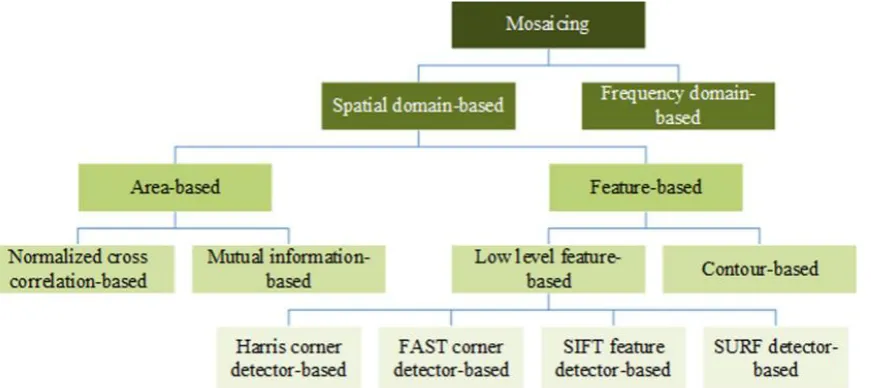
Figure 3 above shows, based on image registration methods, image mosaicing algorithms can be spatial domain-based or frequency domain-based. Spatial domain-based image mosaicing can further be classified into area-based image mosaicing and feature-based image mosaicing. Feature-based image mosaicing can again be subdivided into low level feature-based image mosaicing and contour-based image mosaicing. Low level feature-based mosaicing can be divided into four classes: Harris corner detector-based mosaicing, FAST corner based mosaicing, SIFT feature detector-based mosaicing, and SURF detector-detector-based mosaicing. Figure 4 above shows, based on the image blending methods, mosaicing algorithms can be transition smoothening-based and optimal seam-based. Transition

smoothening-based mosaicing can further be classified into feathering-based, pyramid-based, and gradient-based mosaicing.

IV. FEATURE EXTRACTION

(5)

23 Copyright © 2018. IJEMR. All Rights Reserved.

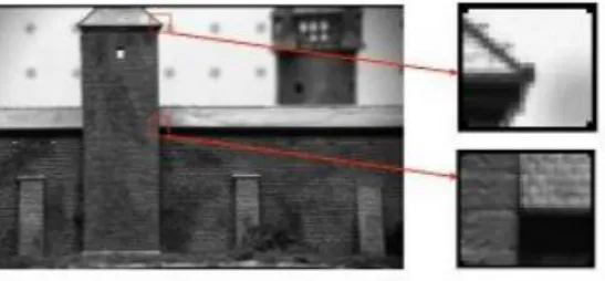
Figure 5 (Left): Patch matching input image 1. Figure 6 (Right): Input image 2.

Figure 7 (Left): Patch matching input image 1. Figure 8 (Right): Input Image 2.

In the example shown above, we can clearly notice that figures 5 and 6 give the best patch match as there is only one patch in figure 6that looks exactly identical to the patch which is given in figure 5.

However, when considering figures 7 and 8, we see a bad patch match as there are numerous identical patches to the patch so given in figure 8. Therefore the conclusion is; exact feature matching cannot be done here because intensities are slightly equal.

Figure 9: Junction of contours corners.

Corners are compared to give a quantitative measurement in order to provide a better feature matching for the pairs of images. Important features of corners are that they are more stable features over changes of viewing angles. The other most important feature of corner is that if there is a corner in an image that its neighbourhood will show an abrupt change in

(6)

24 Copyright © 2018. IJEMR. All Rights Reserved.

V. IMAGE MOSAICING BASED ON

REGISTRATION GROUPING AND

CLASSIFICATION

Other than image registration being considered as an important step in image mosaicing it is also considered the foundation of it. Registration of images coming from different sources (multisource images), which are focused on the same target but produced from different sensors, different perspective as well as different times, computes the optimal geometric transformation by looking into the correspondences between each pair of images. According to Fitzpatrick, Hill and Maurer in [34] who state that this process makes the multi-source images aligned into a common reference frame using the estimated geometric transformations. To the extent that corresponding points from multi-source images are aligned together, the registration is successful. The previously mentioned correspondences can be established in three ways, either by matching templates between images, or by matching features extracted from images, or by utilizing the phase correlation property in the frequency domain.

In the following two subsections the authors discuss different classes of image mosaicing algorithms based on the image registration which are: spatial domain image mosaicing algorithms and frequency domain image mosaicing algorithms.

5.1. Spatial domain image mosaicing algorithms Algorithms in this category use properties of pixels to perform registration, and, thus they are the most direct methods of image mosaicing. A Majority of current and existing image mosaicing algorithms fall into this category.

In accordance to Ghannam and Abbott in their article [60], spatial domain-based image mosaicing can be either area-based or feature-based. Area-based image mosaicing algorithms rely on computation between windows of pixel values in the two images, which need to be mosaicked. The basic approach is to shift the windows of the images relative to each other and see how much the pixels match. Subsequently, transformation parameters are obtained and used to warp and stitch the images. Area-based mosaicing algorithms are often referred to as pixel-based mosaicing, since they use pixel-to-pixel matching, in contradiction to feature-to-feature matching used in the feature-based mosaicing. Two of the most commonly used area-based image mosaicing algorithms are normalized cross correlation-based mosaicing and mutual information-based mosaicing. Both of these techniques provide a measure of image similarity, because larger values of these metrics result from matching areas or windows.

5.1.1. Normalized cross correlation (NCC)-based mosaicing

This technique calculates the similarities between the windows in the two images for each shift. Szeliski defines it as follows in [55].

(1) where;

(2)

(3)

Where and are the mean images of the corresponding windows and as well as for the first and second images respectively. is the number of pixels in the window, is the pixel coordinate in the windows, and is the displacement or shift whereas NCC coefficient is computed. The NCC co-efficient values are always within the range . The shift parameter corresponding to the peak NCC value represents the geometric transformation between the two images. Once geometric transformations are obtained between the image pairs, images are warped in the reference frame, and lastly stitching is performed to generate the final mosaic. Techniques within this category have the strengths of being computationally simple, nonetheless, at the cost of being particularly slow. Furthermore, only when there are significant overlapping between the source images are they capable of performing accurately.

(7)

25 Copyright © 2018. IJEMR. All Rights Reserved.

5.1.2. Mutual information (MI)-based mosaicing Mutual information measures similarity based on the quantity of information shared between two images, in contrast to NCC, which computes similarity

based on image intensity values. MI between two images

and is expressed in terms of entropy as:

(4)

Where and are the entropies of

and , respectively. Entropy is a measure

of variability of a random variable so here,

represents the joint entropy between the two images. Thus variability of is expressed as:

(5)

Where g(s) are the possible gray level values of and accordingly is probability distribution

function of g. similarly, the joint variability of

and is expressed as:

(6)

Where h(s) shows the possible gray level values

of . is the joint probability

distribution function of g and h. Normally, the joint probability distribution between two (2) images is measured as normalized joint histogram of the ray level values. It is observed that the better the alignment between two images, the higher the MI between them. Therefore, two images are geometrically aligned by a transformation if the MI between them is at its maximum for that transformation. Following the obtaining of appropriate transformations between the image pairs, they are then re-projected and stitched to get the final mosaic. These mosaicing methods have the strengths of being less sensitive to lighting and occlusion changes between source images. However, similar to NCC-based techniques, they have the weaknesses of requiring high degree of overlapping between input images and being computationally slow.

Numerous researchers have proposed several techniques to overcome the above mentioned weaknesses. Cesare, Rendas, Allais and Perrier in their research [8] tackled the drawback on MI-based mosaicing algorithms for low overlapping images and proposed a template matching approach with the ability to explicitly acknowledging the plausibility of similarity between distant neighbourhoods and delaying definite block-to-block association to a step that evaluates globally their collective likelihood. Luna, Daul, Blondel, Hernandez-Mier, Wolf and Guillemin all use stochastic gradient optimization along with MI-based similarity measure in their research in order to make the algorithm much faster [53]. As for computational speed and how to increase it, the authors Dame and Marchand in their conference paper [2] employed a B-spline function for normalized mutual probability density. Furthermore, the authors also used Newton‟s method to speed up the estimation of the displacement parameters.

Different from the area-based methods, feature-based mosaicing techniques make use of feature-to-feature matching so as to be able to compute the geometric transformation between a pair of images. Therefore, these methods rely mainly on feature extraction algorithms which can detect salient features from the images. As discussed in [43] by Islam and Kabir; salient features are subsets of the image domain, often in the form of isolated points, continuous curves or connected regions. The general approach is to detect a few corresponding features from the source images, and then estimate homography using the reliable correspondences only. Using the homography matrices images are first warped and then stitched in a common reference coordinate. Since the features are used as the starting point, the overall algorithm will often be as good as the feature extraction algorithm is. Techniques that fall into this category give in general better results than the area-based methods; nonetheless, this is all at a cost of high computation requirement. Depending on the types of features extracted, feature-based mosaicing methods can be classified into low-level feature-based mosaicing and contour-based mosaicing.

5.1.3. Low-level feature-based mosaicing

(8)

26 Copyright © 2018. IJEMR. All Rights Reserved.

the detector must have high repeatability rate, in such a way that same features are detected in the overlapping regions between pair of images, as indicated previously in figures 5, 6, 7 and 8. Popular low-level feature extraction methods used in mosaicing literature include the following:

1. Harris corner detector

2. Features from Accelerated Segment Test (FAST)-based corner detector

3. Scale Invariant Feature Transform (SIFT)-based feature detector

4. Speeded Up Robust Feature (SURF)-based feature detector

Mosaicing algorithms based on these feature extraction techniques are discussed below:

5.1.3.1. Harris corner detector

Harris corner detector detects corner points as robust low-level features from source images. Initially a local detection window in an image is selected. Joshi and Sinha [25] determine as shown below the subsequent variation in intensity that results by shifting the window by a small amount in different direction:

(7)

where is the window function for the detection “window” is the image intensity value at pixel location and

is the shifted intensity with shift. The local texture around pixel is expressed as autocorrelation matrix C as shown below:

(8)

where and are the first derivative of

. Two large eigenvalues for the matrix corresponds to a corner point. The centre point of the window is characterized as corner point. In order to

eliminate the edge points, the authors Gao and Jia in [20] use a “cornerness” measure for more robustness as shown below:

(9)

Where is the trace of and within the range . Corner points ae detected as local maxima or above a predefined threshold . After the Harris corner points are detected from both the images, correspondences are established either by NCC or by any other sum of squared difference (SDD) technique. Subsequently, the geometric motion parameters are computer and images are warped into global reference frame in order to stich them all. Mosaicing algorithms using Harris corner detector are computationally simple and accurate.

Harris corner detector almost always identifies closely crowded features. Nonetheless, Okumura, Raut, Gu, Aoyama and Takaki [37] discuss show how this can be overcome by counting the number of features in the neighbourhood and then exclude some of the points accordingly. A major drawback with the Harris corner detector-based mosaicing technique is that large changes in rotation often generate ghosting in the mosaicing output. Gao and Jia in [20] use a luminance centre-weighting algorithm which is used following a slope clustering algorithm for Harris corner point matching to tackle with this drawback. In addition, another drawback related to the uncertainty is selecting a local detection window, which was handled by Zagrouba, Barhoumi and Amri in [17], where the authors used region segmentation and matching so as to limit the search window to potential homologous points.

5.1.3.2. Feature from Accelerated Segment Test (FAST)-based corner detector

FAST is a corner detector algorithm. Trajkovic and Hedley founded this algorithm in 1998.The detection of corner was prioritized over edges in FAST as corners were found to be the good features to be matched because it shows a two dimensional intensity change, thus well distinguished from the neighbouring points. According to Trajkovic and Hedley the corner detector should satisfy the following criteria:-

I. Consistency & Insensitivity: The detected positions should be consistent, insensitive to the variation of noise, and they should not move when multiple images are acquired of the same scene.

II. Accuracy: Corners should be detected as close as possible to the correct positions.

(9)

27 Copyright © 2018. IJEMR. All Rights Reserved.

In accordance to the FAST algorithm, the candidate is a corner if there exists a set of contiguous pixels in the circle which are all brighter than the intensity of the

candidate pixel minus the threshold, figure 10 shows this clearly.

Figure 10: Candidate feature detection for FAST algorithm [70]. The number is usually chosen as twelve. In

order to increase the speed of FAST algorithm, a corner response function (CRF) is used. The authors in [25] state that CRF gives the numerical value of the „„cornerness” of a corner point based on image intensities in the local neighbourhood. Corners are detected as local maxima for the CRF function computed over the entire image. Following the detection, corner point matching is performed for each pair of frames. Sometimes a Bag-of-Words (BoW) algorithm is used to represent each image as a set of corner descriptors to speed up the matching process as in [65]. Then, homography matrices are computed and finally the images are projected into a common coordinate to get the final mosaic.

A fundamental challenge of the FAST corner detector-based algorithms is choosing an optimal threshold. Nonetheless, Jiao, Zhao and Wu in [28] show that it can be addressed by incorporating a robust threshold selection algorithm. For matching the corner points from successive frames, they further proposed a threshold learning method together with a region-based gray correlation. Other major issue of the FAST-based

algorithms include that which they are not particularly robust to increased degree of variations; for that, extending the sampling area beyond the sixteen pixels around each candidate point. A promising approach is proposed by Wang, Sun and Peng in [70], since it gives the FAST corner points more distinctiveness and, in turn, makes them invariant to larger variations.

5.1.3.3. Scale Invariant Feature Transform (SIFT)-based feature detector

SIFT algorithm is a low-level feature detection algorithm which detects distinctive features also known as „„key-points” from images. The SIFT descriptor is invariant to translations, rotations and scaling transformations in the image domain and robust to moderate perspective transformations and illumination variations. SIFT‟s operation is based on five primary steps which are: scale-space construction, scale-space extrema detection, key-point localization, orientation assignment, and defining key-point descriptors. Lowe [14] mentions that, originally, a scale space is constructed by convolving an image repeatedly using a Gaussian filter with changing scales and grouping the outputs into octaves as shown below:

(10)

Where is the convolution operator, is a Gaussian filter with variable scale , and is the input image. As [14] shows, after the scale space

construction is complete, difference-of-Gaussian (DoG) images are calculated from adjacent Gaussian-blurred images in each octave, as shown below

(11)

After that, candidate key-points are identified as local extrema of DoG images across the scales. The scale

(10)

28 Copyright © 2018. IJEMR. All Rights Reserved.

11 and 12 below. In the following step, as indicated in [14] low contrast key-points and edge response points along the edges are discarded using accurate key-point

localization. The key-points are then assigned one or more orientations based on local image gradient directions as shown below:

(12)

where represents the gradient direction

for . A set of orientation histograms is formed

over the neighbourhoods of each key-point.

Figure 11: Scale space and DoG scale construction [14].

Figure 12: Extrema detection in DoG scale space by looking into 26 neighbours [14].

Gosh, Kaabouch and Fevig in [10] discuss the final step where, a normalized 128-dimensional vector is computed for each key-point as its descriptor. In order to find the original matching key-points from two images, nearest neighbour of a key-point in the first image is identified from a database of key-points for the second image as shown in [50 and 52]. Following the initial matching, RANSAC algorithm is used to remove the outliers and to calculate the transformation parameters between a pair of frames. Lastly, images are warped using the transformation parameters and stitched to generate the mosaic image. SIFT based image mosaicing algorithms are particularly suitable for stitching high resolution images under variety of changes such as rotation, scale, affine and more, nonetheless, high processing time is the expense to be paid.

Several researchers have made variations to the above mentioned SIFT-based mosaicing technique so as to improve its performance even further. Take for example Yao In [38] exploited a deformation vector

propagation algorithm in the gradient domain to reduce the intensity discrepancy between the mosaicked images. Furthermore, Nemra and Aouf in [5] proposed switching between Kanade-Lucas-Tomasi (KLT) tracker and SIFT matching to find the correspondences between successive frames depending on their amount of overlapping. Similarly, a bundle adjustment algorithm along with a modified-RANSAC algorithm capable of developing a probabilistic model is used by Li, Wang, Huang and Zhang in [72] in order to eliminate registration error and make the matching process more accurate.

5.1.3.4. Speeded Up Robust Feature (SURF)-based feature detector

(11)

29 Copyright © 2018. IJEMR. All Rights Reserved.

[23] the Hessian matrix of an image with scale at any point is defined as follows:

(13)

where and

respectively. While calculating Hessian matrix at each pixel, the Gaussian filter operations are approximate by

operations using box filter as figure 13, 14 and 15 below show:

Figure 13 (Left): Approximation of Gaussian second order partial derivatives in [45]. Figure 14 (Centre): Approximation of Gaussian second order partial derivatives in [45]. Figure 15 (Right): Approximation of Gaussian second order partial derivatives in [45].

The response at each pixel is computed as the determinant of the Hessian matrix. Afterwards, for non-maxima suppression, a thresholding and a 3 x 3 x 3 local maxima detection window are used. The local maxima are then interpolated in scale space to achieve key-points with their location and scale values. In order to assign orientation for each key-point, Haar-wavelet responses are calculated within a circular neighbourhood around each key-point. A vector is then formed by totalling up all the responses within a 60-degree window. The longest vector is assigned as orientation to the key-point. So as to be able to assign descriptor vector to each key-point, a square neighbourhood region around the key point is chosen and selected. As shown by Bind in [69] it is then split into smaller sub-regions. Total of the Haar-wavelet responses from all the sub-regions are then used to generate a 64 dimensional descriptor vector. After finding the matching key-points from a pair of images, RANSAC algorithm is used to eliminate false matches as well as to calculate the homography matrices. Once homography matrices are achieved, images are warped and stitched to get the final mosaic. SURF-based mosaicing methods are generally faster than SIFT-based methods. Nonetheless, under certain variations such as more particularly color, illumination as well as some affine transformation they perform poorly.

The process of determining the SURF descriptors as mentioned above has sometimes been modified by some authors. Such as take for example; Geng, He and Song in [45] the local maxima is searched beyond a 3 x 3 x 3 neighbourhood in the present scale and two immediately adjacent scales in order to make the feature descriptors more distinctive. In [58], the authors Wen, Hui, Jiaju, Yanyan and Haeusler proposed dividing the SURF descriptor window into eight

sub-regions while assigning descriptor vector. This method increases the matching speed at the expense of increased number of false matches. Nonetheless, the authors in their research show that the use of RANSAC guarantees elimination of most of those incorrect matches. Often multiple low-level feature extraction techniques are used together in image mosaicing algorithms in order to use their respective benefits. The authors Peng and Hongbing in [36] as well as Zhu and Ren in [33] both used Harris corner detector and SIFT detector in their feature-based mosaicing algorithm. Joshi and Sinha [24] proposed a mosaicing algorithm which uses both Harris corner detector and SURF detector for extracting distinctive features from source images as well. Furthermore, feature-based mosaicing algorithm proposed by Bind, Muduli and Pati in [68] used a combination of SIFT and SURF based feature detector to detect interest points from images.

5.1.4. Contour-based mosaicing

(12)

30 Copyright © 2018. IJEMR. All Rights Reserved.

mosaicing algorithms. Nonetheless, they are most particularly suitable to work under larger and complicated motion parameters, and even under multi-layer registration. A number of notable contributions in high-level feature-based mosaicing include those in [32], where the authors Xiao, Zhang and Shah used a wide baseline algorithm together with an adaptive region expansion method to achieve robust registration using high-level features. Furthermore, Prescott, Clary, Weit, Pan and Huang proposed extracting regions of image structures using a threshold method and then computing area-based similarity matching for registration in [30]. The authors Deshmukh and Bhosle used contour

extraction using a segmentation algorithm, followed by finding their centroids for image registration in [40]. 5.2. Frequency domain image mosaicing algorithms

Unlike spatial domain-based image mosaicing algorithms, tehniques classified in this category need and require computation in the frequency domain so as to find the optimal transformation parameters between a pair of images. These algorithms use the property of phase correlation for registering images. Let and

are two images having some overlapping areas.

Let us further make an assumption that is the translation between the images. Therefore,

(14) The corresponding Fourier transforms and are related by:

(15) The cross-power spectrum of the images is defined as:

(16)

Where is the complex conjugate of

. The shift theorem guarantees that the phase of

he cross-power spectrum is equivalent to the phase difference between the images. could be solved

in two different ways. One way is to work directly in the frequent domain. Nonetheless, this method is sensitive to

noise. A much better approach would be to take inverse Fourier transform of equation 16 and get an impulse function , which is approximately zero everywhere except at the displacement , figure 16, 17 and 18 below show the use of cross-power spectrum to detect transformation:

Figure 16: Source images with displacement between them [18].

Figure 17 (Left & Centre):Spectrum of images in figure 16 [18].

(13)

31 Copyright © 2018. IJEMR. All Rights Reserved.

With the displacement (translational) parameters the two images are warped and finally stitched to get a mosaic. Mosaicing algorithms based on this method are normally efficient because of the use of shift property of Fourier transform and the use of fast Fourier transform (FFT). Nonetheless, they suffer from being overly sensitive to noise. Furthermore, accurate registration most of the time requires significant overlapping between source images. The above explained technique of image mosaicing has sometimes been modified in order to make it suitable for handling transformations other than translation as shown in [18][27][9]. Yang, Wei, Zhang and Tang in [18] use a log-polar transformation to find the scale and translational parameters. In [27] the authors propose a two-step technique. The first step calculates the rotation angle by finding the maximum peak while rotating the target image with an incremental angle. Using the computed rotation angle and phase correlation, the second step determines the translational displacement. The authors in [9],suggested changing the rotation and scale parameters to translational parameters using Fourier–Mellin transform.

VI. IMAGE MOSAICING BASED ON

BLENDING GROUPING AND

CLASSIFICATION

Image blending is an important step in order to successfully implement masaicing, similar to registration. Stitching multiple images together to create a seamless mosaic requires the use of a suitable blending algorithm. Blending is often referred to as photometric registration, which is vital to equalize color and luminance appearance in a composite image. There are a number of reasons such as: variation in scene illumination, difference in camera exposure, geometric misalignments, presence of moving objects between frames and more which may lead to inconsistencies in the final mosaic image. By selecting an appropriate blending algorithm

the visibility of such inconsistencies can be minimized. This way, giving the final mosaic a consistent global appearance and it would be visibly free of annoying seams. The following two subsections discuss the classification of image mosaicing algorithms based on the image blending techniques used by them.

6.1. Image mosaicing algorithms using transition smoothing-based blending

Mosaicing algorithms within this category by smoothing the common overlapping regions of the combined image attempt to minimize the visibility of seams. The information of the overlapping region between two images is fused in such a way that the boundaries of the images involved become imperceptible. In [54] the authors explain that; even though a totally indistinguishable transition may be achieved, the content and coherency of the overlapping region is not guaranteed, as the information is fused without taking into account the content of the scene. Therefore, most often, these mosaicing techniques generate mosaic with blurry transitions in the boundary regions. Popular techniques which use transition smoothing for their blending operation include gradient-based blending, feathering and pyramid blending. Mosaicing algorithms based on these methods are discussed briefly as follows. 6.1.1. Mosaicing algorithms using feathering-based blending

Mosaicing algorithms within this category perform blending operation by taking an average value in each pixel of the overlapping region. However, the simple average technique fails when exposure differences, misalignments and presence of moving object are very obvious in the input images. A superior technique is to use weighted averaging along with a distance map. Pixels near the centre of an image are weighted heavily and those near the edges are weighted lightly. As [55] shows this is done by calculating a distance map in terms of Euclidean distance of each valid pixel known as mask from its nearest invalid pixel as shown below:

(17)

wherẽ are the wrapped images and are the weights of the images. Finally, the mosaic image is generated as a weighted combination of the input

images. Figure 19 and 20 below show an example of composite images formed of six color images using simple average blending and fathering.

(14)

32 Copyright © 2018. IJEMR. All Rights Reserved.

Mosaicing algorithms which use the previously mentioned method perform reasonably well under exposure differences. Nonetheless, in practice it is difficult to achieve a balance between smoothing out low-frequency exposure differences and the preservation of sharp enough transitions in order to prevent blurring. In addition, these methods suffer from ghosting artefacts. There are a number of examples of mosaicing techniques using feathering-based blending including those which are discussed in [53 and 68], where the authors use alterations of the above mentioned technique in order to find the weight of images in the overlapping regions. In

[15] the authors used weighted average of the pixel color values in the overlapping region, while in [72]; the previously mentioned weight is measured by calculating the distance of the overlapping pixels from the borders of the left and right images.

6.1.2. Mosaicing algorithms using pyramid-based blending

These mosaicing algorithms convert the input images into band-pass pyramids in an attempt to perform the blending operation in a more robust way, these as shown in figure 21 and 22 below.

Figure 21 (Left): Low-pass pyramid [50]. Figure 22 (Right): Band-pass pyramid [50].

Mask image associated with each source image is then created. Mask creation can be made automatic by using grassfire transform as used in [75]. Then as shown in [55] the mask image is converted into a low-pass pyramid by using a Gaussian kernel. The resultant

blurred and subsampled masks are treated as weights to perform per-level feathering. The final mosaic is then achieved by interpolating and summing up the results from per-level feathering as:

(18)

Where and are the Laplacian pyramids of the warped source images and

. is the Gaussian pyramid of the mask

image and is the Laplacian pyramid of the output image .

As proposed in [42], we see that sometimes, all the strips are combined in a single blending step when pyramids for multiple narrow strips are required. The authors Pandey and Pati in [6] show that algorithms using the above tehcnique achieve reasonable balance between smoothing out low frequency components and preserving sharp enough transitions to prevent blurring. Edge duplication is also eliminated noticeably using these techniques. Nonetheless, double contouring and ghosting effects become significant when the registration error is significant.

6.1.3. Mosaicing algorithms using gradient-based blending

Another group of transition smoothening technique is based on gradient domain blending. These techniques are based on the idea that by suitably mixing the gradient of images, it becomes possible to mosaic image regions convincingly. Generally, the gradients across seams are set to zero for smoothing out the color differences. Since humans are more sensitive to

gradients than image intensities, mosaicing techniques using this method generate visually more pleasant results compared to the other two methods discussed before. Nonetheless, working exclusively in the gradient domain needs and requires higher computational resources to deal with large data sets. In addition, the alignment of images through registration needs to be almost perfect for best performance.

(15)

6.2. Image mosaicing algorithms using optimal seam-based blending

This type of mosaicing algorithms looks for optimal seams in the joining boundaries between the images in an attempt to minimize the visibility of seams. The objective of optimal seam method is to allocate the optimal location of a seam line by looking into the overlapping region between a pair of images. The seam line placement should be such that it minimizes the photometric differences between the two sides of the line. At the same time the seam line should be able to determine the contribution of each of the images in the final mosaic. Once the placement and the contribution information are obtained, each image is copied to the corresponding side of the seam. When the difference between the two images on the seam line is zero, no seam gradients are produced in the mosaic. Different from the mosaicing techniques using transition smoothing-based blending, optimal seam-based mosaicing algorithms consider the information content of the scene in the overlapping region, allowing to deal with problems like moving objects or parallax. Nonetheless, no information is fused in the overlapping region, therefore, the transition between the images can be easily noticeable when there are global intensity or exposure difference between the frames. Different optimal seam finding methods have been used in mosaicing literature. Given for example, in [41] the authors El-Shaban, Izz, Kaheel and Refaat use a modified region-of difference technique. In [46], Gracias, Mahoor, Negahdaripour and Gleson proposed the use of an algorithm based on watershed segmentation and graph cut optimization. Another technique based on dynamic programming and grey relational analysis is used by Wen and Zhou in [26].

VII. CONCLUSION

In the field of computer vision, image mosaicing is considered an important task. The Success of a mosaicing algorithm depends mainly on registration and blending techniques as shown throughout this paper, which provides an in-depth classification of image mosaicing techniques and approaches based on image registration and blending algorithms. Furthermore to providing the description of the different categories, this paper discusses the strengths and weaknesses of each category. It is obvious from the discussion that there is no single best image mosaicing group or category. At the same time, the continuous advent of new mosaicing techniques and approaches in recent years makes it absolutely difficult to select an appropriate and suitable mosaicing algorithm for a specific purpose. Hence, this paper aims at providing a guide for selecting a suitable mosaicing technique for a specific application. Although an extensive research has been done in the area of mosaicing, there are still a number of problems to be addressed and discussed further more. Such as for example; the processing time and mosaicing in the presence of images with significant parallax both are

challenges. All mosaicing approaches and methods are time consuming and cannot run on low power and low frequency devices. The future researches can be directed as addressing those issues mentioned above.

REFERENCES

[1] A. Behrens, M. Guski, T. Stehle, S. Gross, & T. Aach. (2010). Intensity based multi-scale blending for panoramic images in fluorescence endoscopy. IEEE International Symposium on Biomedical Imaging: From Nano to Macro, 1305–1308.

[2] A. Dame & E. Marchand. (2010). Video mosaicing using a mutual information-based motion estimation process. IEEE International Conference on Image Processing (ICIP), 1493–1496.

[3] A. Levin, A. Zomet, S. Peleg, & Y. Weiss. (2004). Seamless image stitching in the gradient domain. Computer Vision-ECCV, 377–389.

[4] A. Nasibov, H. Nasibov, & F. Hacizade. (2009). Seamless image stitching algorithm using radiometric lens calibration for high resolution optical microscopy. International Conference on Soft Computing, Computing with Words and Perceptions in System Analysis, Decision and Control, 1–4.

[5] A. Nemra & N. Aouf. (2009). Robust invariant automatic image mosaicing and super resolution for UAV mapping. International Symposium on Mechatronics and its Applications, 1–7.

[6] A. Pandey & U.C. Pati. (2013). A novel technique for non-overlapping image mosaicing based on pyramid method. IEEE India Conference (INDICON), 1–6. [7] C. D. Kuglin & D. C. Hines. (1975). The phase correlation image alignment method.. IEEE International Conference on Cybernet. Society, New York, 163- 165.

[8] C. de Cesare, M.-J.Rendas, A.-G. Allais, & M. Perrier. (2008). Low overlap image registration based on both entropy and mutual information measures. OCEANS, 1–9.

[9] C. Wang, Y. Cheng, & C. Zhao. (2009). Robust

subpixel registration for image mosaicing. Chinese

Conference on Pattern Recognition, 1–5.

[10] D. Ghosh, N. Kaabouch, & R.A. Fevig. (2014). Robust spatial-domain based super resolution mosaicing of cubesat video frames: Algorithm and evaluation. Computer and Information Science, 7(2), 68-81.

[11] D. I. Barnea, & H. F. Silverman. (1972). A class of algorithms for fast digital registration. IEEE Transaction on Computer, C-21, 179- 186.

[12] D. Liqian & J. Yuehui. (2010). Moon landform images fusion and Mosaic based on SIFT method. International Conference on Computer and Information Application (ICCIA), 29–32.

(16)

[14] D.G. Lowe. (2004). Distinctive image features from scale-invariant keypoints. International Journal of Comput. Vision, 60, 91–110.

[15] D.K. Jain, G. Saxena, & V.K. Singh. (2012). Image mosaicing using corner techniques. International Conference on Communication Systems and Network Technologies (CSNT), 79–84.

[16] E. Zagrouba, W. Barhoumi, & S. Amri. (2009). An efficient image-mosaicing method based on multifeature matching. Mach. Vis. Appl. 20, 139–162.

[17] F. Yang, L. Wei, Z. Zhang, H. Tang, Image mosaic based on phase correlation and Harris operator. Journal of Computational Information System, 8(6), 2647–2655. [18] F. Zhao, Q. Huang, & W. Gao. (2006). Image matching by normalized cross-correlation. IEEE International Conference on Acoustics, Speech and Signal Processing, 729-732.

[19] G. Gao & K. Jia. (2007). A new image mosaics algorithm based on feature points matching. International Conference on Innovative Computing, Information and Control, 471–471.

[20] G. Guandong & J. Kebin. (2007). A new image mosaics algorithm based on feature points matching, in: International Conference on Innovative Computing, Information and Control, 471–471.

[21] G. Jun-Hui, Z. Jun-Hua, A. Zhen-Zhou, Z. Wei-Wei, & L. Hui-Min. (2012). An approach for X-ray image mosaicing based on Speeded-up robust features, in: International Conference on Wavelet Active Media Technology and Information Processing (ICWAMTIP), 432–435.

[22] H. Bay, T. Tuytelaar &, L. Van Gool. (2006). Surf: speeded up robust features. Computer Vision–ECCV, 404–417.

[23] H. Joshi & K. Sinha. (2013). Novel techniques image mosaicing based on image fusion using harris aand SURF. International Conference on Computer Science and Information Technology, 1-11.

[24] H. Joshi & M.K. Sinha. (2013). A survey on image mosaicing techniques. International Journal of Advanced Research in Computer Engineering & Technology, 2(2), 2013.

[25] H. Wen & J. Zhou. (2008). An improved algorithm for image mosaic. International Symposium on Information Science and Engineering, 497–500.

[26] H. Xie, N. Hicks, G.R. Keller, H. Huang, & V. Kreinovich. (2003). An IDL/ENVI implementation of the FFT-based algorithm for automatic image registration. Comput. Geosci. 29(8), 1045–1055.

[27] J. Jiao, B. Zhao, & S. Wu. (2011). A speed-up and robust image registration algorithm based on fast. IEEE International Conference on Computer Science and Automation Engineering (CSAE), 160–164.

[28] J. Prescott, M. Clary, G. Wiet, T. Pan, & K. Huang. (2006). Automatic registration of large set of microscopic images using high-level features. IEEE International Symposium on Biomedical Imaging: Nano to Macro, 1284–1287.

[29] J. Seokhee & G.J. Kim. (2007). Mosaicing a wide geometric field of view for effective interaction in

augmented reality. IEEE and ACM International Symposium on Mixed and Augmented Reality, 265–266. [30] J. Xiao, Y. Zhang, & M. Shah. (2005). Adaptive region-based video registration. IEEE Workshops on Application of Computer Vision, 215-220.

[31] J. Zhu & M. Ren. (2014). Image mosaic method based on SIFT features of line segment. Computational and Mathematical Methods in Medicine, 1-11.

[32] J.M. Fitzpatrick, D.L. Hill, & C.R. Maurer Jr. (2004). Image registration, Handbook of Medical Imaging, 2, 447–513.

[33] K. Berberidis & I. Karybali. (2002). A new efficient cross-correlation based image registration technique with improved performance. Proceedings of the European Signal Processing Conference, 3–6.

[34] K. Peng & M. Hongbing. (2011). An automatic airborne image mosaicing method based on the SIFT feature matching. International Conference on Multimedia Technology (ICMT), 155–159.

[35] K.-I. Okumura, S. Raut, Q. Gu, T. Aoyama, T. Takaki, & I. Ishii. (2013). Real-time feature based video mosaicing at 500 fps. International Conference on Intelligent Robots and Systems (IROS), 2665–2670. [36] L. Yao. (2008). Image mosaic based on SIFT and deformation propagation. IEEE International Symposium on Knowledge Acquisition and Modeling Workshop, 848–851.

[37] Lisa G. Brown. (1992). A survey of image registration techniques. ACM Computing Surveys, 24(4), 325- 376.

[38] M. Deshmukh & U. Bhosle. (2011). A survey of image registration, International Journal of Image Processing (IJIP), 5(3), 245-269.

[39] M. El-Saban, M. Izz, A. Kaheel, & M. Refaat. (2011). Improved optimal seam selection blending for fast video stitching of videos captured from freely moving devices. IEEE International Conference on Image Processing (ICIP), 1481–1484.

[40] M. Vivet, S. Peleg, & X. Binefa. (2011). Real-time stereo mosaicing using feature tracking. IEEE International Symposium on Multimedia (ISM), 577– 582.

[41] M.B. Islam & M.M.J. Kabir. (2013). A new feature-based image registration algorithm. Computer Technology and Application, 4, 79–84.

[42] M.H.M. Patel, A.P.P.J. Patel, & A.P.M.S.G. Patel. (2012). Comprehensive study and review of image mosaicing methods. International Journal of Engineering Research and Technology, 1(9), 1-7. [43] N. Geng, D. He, & Y. Song. (2012). Camera image mosaicing based on an optimized SURF algorithm, Indonesian Journal of Electrical Engineering, 10(8), 2183–2193.

(17)

International Journal of Computational Engineering, 3(4), 106-109.

[47] P. Kolonia. (1994, Jan). When more is better. Popular Photography, 58(1), 30-34.

[48] P. Liang, X. Zhiwei, & D. Jiguang. (2010). Joint edge detector based on Laplacian pyramid. International Congress on Image and Signal Processing (CISP), 978– 982.

[49] P.J. Burt. (1988). Smart sensing within a pyramid vision. Proceedings of the IEEE, 76(8), 1006-1015. [50] R. Abraham & P. Simon. (2013). Review on mosaicing techniques in image processing. International

Conference on Advanced Computing and

Communication Technologies (ACCT), 63–68.

[51] R. Miranda-Luna, C. Daul, W.C. Blondel, Y. Hernandez-Mier, D. Wolf, & F. Guillemin. (2008). Mosaicing of bladder endoscopic image sequences: distortion calibration and registration algorithm, IEEE Transactions on Biomedical Engineering, 55, 541–553. [52] T. Vercauteren, A. Perchant, X. Pennec, & N. Ayache. (2005). Mosaicing of confocal microscopic in vivo soft tissue video sequences. Medical Image

Computing and Computer-Assisted Intervention

(MICCAI), 753–760.

[53] R. Szeliski. (2006). Image alignment and stitching: A tutorial. Foundations and Trends in Computer Graphics and Vision, 2(1), 1–104.

[54]M. J. Black & A. D. Jepson. (1998). Eigen tracking: Robust matching and tracking of articulated objects using a view-based representation. International Journal of Computer Vision, 26(1), 63–84.

[55] R. Szeliski, M. Uyttendaele, & D. Steedly. (2011). Fast poisson blending using multisplines. International Conference on Computational Photography (ICCP), 1–8. [56] R. Wen, C. Hui, L. Jiaju, X. Yanyan, & R. Haeusler. (2009). Mosaicing of microscope images based on SURF. International Conference on Image and Vision Computing New Zealand, 271–275.

[57] S. C. Chen. (1995). Quicktime VR: An image-based approach to virtual environment navigation. Interactive Technology, SIGGRAPH, 29–38.

[58] S. Ghannam & A.L. Abbott. (2013). Cross correlation versus mutual information for image

mosaicing. International Journal of Advanced Computer Science and Applications, 4(11), 94-102.

[59] S.Z. Kovalsky, G. Cohen, & J.M. Francos. (2007). Registration of joint geometric and radiometric image deformations in the presence of noise. IEEE/SP Workshop on Statistical Signal Processing, 561–565. [60] Soo-Hyun CHO, Yun-Koo CHUNG, & Jae Yeon LEE. (2003). Automatic image mosaic system using image feature detection and taylor series, In Proceedings of the 7th International Conference on Digital Image Computing: Techniques and Applications, Sydney, Australia, 549-556.

[61] T. Botterill, S. Mills, & R. Green. (2010). Real-time aerial image mosaicing. International Conference of Image and Vision Computing New Zealand (IVCNZ), 1– 8.

[62] T. Vercauteren, A. Meining, F. Lacombe, & A. Perchant. (2008). Real time autonomous video image registration for endomicroscopy: fighting the compromises. Biomedical Optics (BiOS), 68610C– 68610C-8.

[63] X. Wang, J. Sun, & H.-Y. Peng. (2012). Efficient panorama mosaicing based on enhanced FAST and graph cuts. Recent Advances in Computer Science and Information Engineering, 128, 757–762.

[64] Y. Lei, W. Xiaoyu, Z. Jun, & L. Hui. (2011). A research of feature-based image mosaic algorithm. International Congress on Image and Signal Processing (CISP), 846–849.

[65] Y. Li, Y. Wang, W. Huang, & Z. Zhang. (2008). Automatic image stitching using sift. International Conference on Audio, Language and Image Processing, 568–571.

[66] Y. Shum & R. Szeliski. (1998). Construction and refinement of panoramic mosaics with global and local alignment. International Conference on Computer Vision, 953–958.

[67] Y. Xiong. (2009). Eliminating ghosting artifacts for panoramic images. IEEE International Symposium on Multimedia, 432–437.