Sparse Estimation in Ising Model via Penalized Monte Carlo
Methods
B la ˙zej Miasojedow [email protected]
Institute of Applied Mathematics and Mechanics University of Warsaw
ul. Banacha 2, 02-097, Warszawa, Poland and
Institute of Mathematics Polish Academy of Sciences
ul. ´Sniadeckich 8, 00-656 Warszawa
Wojciech Rejchel [email protected]
Faculty of Mathematics and Computer Science Nicolaus Copernicus University
ul. Chopina 12/18, 87-100 Toru´n, Poland and
Institute of Applied Mathematics and Mechanics University of Warsaw
ul. Banacha 2, 02-097, Warszawa, Poland
Editor:Sara van de Geer
Abstract
We consider a model selection problem in high-dimensional binary Markov random fields. The usefulness of the Ising model in studying systems of complex interactions has been confirmed in many papers. The main drawback of this model is the intractable norming constant that makes estimation of parameters very challenging. In the paper we propose a Lasso penalized version of the Monte Carlo maximum likelihood method. We prove that our algorithm, under mild regularity conditions, recognizes the true dependence structure of the graph with high probability. The efficiency of the proposed method is also investigated via numerical studies.
Keywords: Ising model, Monte Carlo Markov chain, Markov random field, model selec-tion, Lasso penalty
1. Introduction
A Markov random field is an undirected graph (V, E), where V = {1, . . . , d} is a set of vertices and E⊂V ×V is a set of edges. The structure of this graph describes conditional independence among subsets of a random vector Y = (Y(1), . . . , Y(d)), where a random variable Y(s) is associated with a vertex s ∈ V. Finding interactions between random variables is a central element of many branches of science, for example biology, genetics, physics or social network analysis. The goal of the current paper is to recognize the structure of a graph on the basis of a sample consisting of nindependent observations. We consider
c
the high-dimensional setting, i.e. the number of verticesdcan be comparable or larger than the sample sizen.It is motivated by contemporary applications of Markov random fields in the above-mentioned places, for instance gene microarray data.
The Ising model (Ising, 1925) is an important example of a mathematical model that is often used to explain relations between discrete random variables. In the literature one can find many papers that argue for its effectiveness in recognizing the structure of a graph (Ravikumar et al., 2010; H¨ofling and Tibshirani, 2009; Guo et al., 2010; Xue et al., 2012; Jalali et al., 2011). This model also plays a key role in our paper. On the other hand, the Ising model is an example of an intractable constant model that is the joint distribution of Y is known only up to a norming constant and this constant cannot be calculated in practice.
Thus, there are two main difficulties in the considered model. The first one is the high-dimensionality of the problem. The second one is the intractable norming constant. To overcome the first obstacle we apply a well-known Lasso method (Tibshirani, 1996). The properties of this method in model selection are deeply studied in many papers that mainly investigate linear models or generalized linear models (Bickel et al., 2009; B¨uhlmann and van de Geer, 2011; Huang and Zhang, 2012; van de Geer, 2008; Ye and Zhang, 2010; Zhao and Yu, 2006; Zhou, 2009). However, it is not difficult to find papers that describe properties of Lasso estimators in more complex models, for instance Markov random fields (Banerjee et al., 2008; B¨uhlmann and van de Geer, 2011; Ravikumar et al., 2010; H¨ofling and Tibshirani, 2009; Guo et al., 2010; Xue et al., 2012) that are considered in this paper. There are many approaches trying to overcome the second obstacle that is the intractable norming constant. For instance, in Ravikumar et al. (2010) one proposes to performd regu-larized logistic regression problems. This idea is based on the fact that the norming constant reduces, if one considers the conditional distribution instead of the joint distribution in the Ising model. This simple fact is at the heart of the pseudolikelihood approach (Besag, 1974) that is replacing the likelihood (that contains the norming constant) by the product of conditionals (that do not contain the norming constant). This idea is widely applied in the literature (H¨ofling and Tibshirani, 2009; Guo et al., 2010; Xue et al., 2012; Jalali et al., 2011) to study model selection properties of high-dimensional Ising models. However, this approach works well only if the pseudolikelihood is a good approximation of the likelihood. In general, it depends on the true structure of a graph. Namely, if this structure of the graph is sufficiently simple (examples of different structures can be found in section 5.1), then the product of conditionals should be close to the joint distribution. However, in practice this knowledge is unavailable. Another approach is described in Banerjee et al. (2008). It adapts the method that estimates the precision matrix in gaussian graphical models to the binary case. In the current paper we propose the approach to the norming constant problem that relates to Markov chain Monte Carlo (MCMC) methods. Namely, the norming constant is approximated using the importance sampling technique. This method is independent of the unknown complexity of the estimated graph. It is sufficient that the size of a sample used in importance sampling is sufficiently large to have good approximation of the likelihood.
example, Honorio (2012) and Atchad´e et al. (2017) analyzed stochastic versions of proxi-mal gradient algorithms. Both papers derive nonasymptotic bounds between the output of the algorithm and the true minimizer of the cost function. However, in the current paper we focus on model selection properties of MCMC methods. We investigate them in the high-dimensional scenario and compare to the existing methods that are mentioned above. Model selection for undirected graphical models means finding the existing edges in the “sparse” graph that is a graph having relatively few edges (comparing to the total number of possible edges d(d2−1) and the sample size n).
The paper is organized as follows: in the next section we describe the Ising model and our approach to the problem that relates to minimization of the penalized MCMC approximation of the likelihood. The literature concerning this topic is also discussed. In section 3 we state main theoretical results. Details of efficient implementation are given in section 4, while the results of numerical studies are presented in section 5. The conclusions can be found in section 6. Finally, the proofs are postponed to appendices A and B.
2. Model description and related works
In this section we introduce the Ising model and the proposed method. It also contains a review of the literature relating to this problem.
2.1. Ising Model and undirected graphs
Let (V, E) be an undirected graph that consists of a set of vertices V and a set of edgesE.
The random vector Y = (Y(1), Y(2), . . . , Y(d)), that takes values in Y, is associated with this graph. In the paper we consider a special case of the Ising model thatY(s) ∈ {−1,1}
and the joint distribution ofY is given by the formula
p(y|θ?) = 1
C(θ?)exp X
r<s
θ?rsy(r)y(s) !
, (1)
where the sum in (1) is taken over such pairs of indices (r, s)∈ {1, . . . , d}2 that r < s.The
vectorθ? ∈Rd(d−1)/2 is a true parameter and C(θ?) is a norming constant, i.e.
C(θ?) =X y∈Y
exp X
r<s
θrs? y(r)y(s) !
.
The norming constant is a finite sum but it consists of 2delements that makes it intractable even for a moderate size of d.
For convenience, we denote J(y) = (y(r)y(s))r<s,so
p(y|θ?) = 1
C(θ?)exp
(θ?)0J(y).
Remark 1 The model (1) is a simplified version of the Ising model, for instance we omit an external field in (1). We have decided to restrict to the model containing only parameters
The Ising model has the following property: vertices r and s are not connected by an edge (i.e. θ?rs = 0) means that variables Y(r) and Y(s) are conditionally independent given the other vertices. Therefore, we recognize the structure of the graph (its edges) by estimating the parameterθ?.Assume thatY1, . . . , Ynare independent random vectors from the model (1). Then the negative log-likelihood is
`n(θ) =− 1
n
n X
i=1
θ0J(Yi) + logC(θ). (2)
The second term in (2) contains the norming constant so we cannot use (2) to estimateθ?.To overcome this problem one usually replaces the negative log-likelihood by its approximation and estimates θ? using the minimizer of this approximation. In the current paper the approximation of (2) is based on Monte Carlo (MC) methods. Suppose that h(y) is an importance sampling distribution and note that
C(θ) =X y∈Y
expθ0J(y)=X y∈Y
exp [θ0J(y)]
h(y) h(y) =EY∼h
exp [θ0J(Y)]
h(Y) (3)
for each θ.An MC approximation of the norming constant is
1
m
m X
k=1
exp
θ0J(Yk)
h(Yk) , (4)
whereY1, . . . , Ym is a sample drawn fromhor, which is more realistic and is considered in the current paper, Y1, . . . , Ym is a Markov chain with h being a density of its stationary distribution. Thus, the MCMC approximation of (2) is
`mn(θ) =−1 n
n X
i=1
θ0J(Yi) + log 1
m
m X
k=1
expθ0J(Yk)
h(Yk) !
. (5)
A natural choice of the importance sampling distribution is h(y) =p(y|ψ) for some param-eter ψ.It leads to
`mn(θ) =−1 n
n X
i=1
θ0J(Yi) + log 1
m
m X
k=1
exph(θ−ψ)0J(Yk)i !
+ log(C(ψ)). (6)
The last term in (6), that contains the unknown constant C(ψ),does not depend on θ, so it can be ignored while minimizing (6).
Our goal is selecting the true model (recognizing edges of a graph) in the high-dimensional setting. It means that the number of verticesdcan be large. In fact, it can be greater than the sample size, i.e. d = dn n. To estimate the vector θ? we use penalized empirical risk minimization. The natural choice of the penalty would be thel0-penalty, but it makes
the procedure nonconvex and computationally expensive even for moderate values ofd.To avoid such problems, we use the Lasso penalty and minimize a function
where |θ|1 = P
r<s|θrs| and λmn >0 is a smoothing parameter, that is a balance between minimizing the MCMC approximation and the penalty. We denote the minimizer of (7) by ˆ
θmn.Notice that the function (7), that we minimize, is convex inθ,because the Lasso penalty as well as the MCMC approximation (6) are convex function in θ.The latter follows from the fact that the Hessian of `mn(θ),that is given explicitly in (19), is a weighted covariance matrix with positive weights that sum up to one. Convexity of the problem is important from the practical and theoretical point of view. First, every minimum of a convex function is the global minimum, so there are no local minimum problems. Second, convexity is also utilized in the proofs of the results contained in the paper. In further parts of the paper we study properties of ˆθnm in model selection.
2.2. Related works
Model selection in the high-dimensional Ising model is a popular topic and many papers investigating this problem using different methods can be found in the literature (Banerjee et al., 2008; Bresler et al., 2008; Lee et al., 2006; Ravikumar et al., 2010; H¨ofling and Tibshirani, 2009; Guo et al., 2010; Xue et al., 2012; Jalali et al., 2011). The significant part of them uses the pseudolikelihood approximation with the Lasso penalty. For instance, Ravikumar et al. (2010) applies it by consideringdlogistic regression problems. They prove that this algorithm is model selection consistent, if some regularity conditions are satisfied. These conditions are similar to the “irrepresentable conditions” (Zhao and Yu, 2006), that are sufficient to prove an analogous property in the linear model. The pseudolikelihood method with the Lasso as a “joint” procedure is proposed in H¨ofling and Tibshirani (2009). Moreover, in the same paper one also proposes an “exact” algorithm, that minimizes the negative log-likelihood with the Lasso penalty. However, this procedure also bases on the pseudolikelihood approximation. Model selection consistency of the latter algorithm has not been studied yet. The former procedure has this property, that is showed in Guo et al. (2010) provided that conditions similar to Ravikumar et al. (2010) are satisfied. In Xue et al. (2012) the Lasso penalty is replaced by the SCAD penalty (Fan and Li, 2001) and theoretical properties of this algorithm are studied. In Jalali et al. (2011) one replaces restrictive irrepresentable conditions by weaker restricted strong convexity and smoothness conditions (Negahban et al., 2009) and proves model selection consistency of an algorithm that joints ideas from Ravikumar et al. (2010) and Zhang (2009). Namely, it performs
d separate logistic regression problems with the forward-backward greedy approach. The algorithm described in Banerjee et al. (2008) is also based on the likelihood approximation with the Lasso penalty. However, it does not apply the pseudolikelihood method. Using the determinant relaxation (Wainwright and Jordan, 2006) it treats the problem of model selection in discrete Markov random fields analogously to the continuous case.
are weaker than their analogs from the above-mentioned papers. The detailed comparison is given after Corollary 3 in section 3.
Moreover, the advantage of our algorithm is that the MCMC approach allows us to approximate the norming constant with an arbitrary precision. The approximation error of other methods is given by the problem/data. It depends on the unknown structure of a graph and a user cannot improve it. In our approach a user can improve approximation by increasing the length of simulation, using the MCMC algorithm tailored to the problem. The obvious drawback of our approach is the need of additional simulations to obtain the MCMC sample. It makes our procedure computationally more complex, but at the same time more accurate in selecting the true model.
2.3. Notation
In further parts of the paper we need few notations. Most of them are collected in this subsection.
For simplicity, we write ˆθand λinstead of ˆθmn and λmn,respectively. Besides, we denote the number of estimated parameters in the model by ¯d=d(d−1)/2.Nonzero coordinates of θ? are collected in the setT, andTc is a completion of T. Besides, ¯d
0 =|T|denotes the
number of elements in the set T.
For a vector awe denote itsl∞-norm by|a|∞= max
k |ak|and a
⊗2=aa0.The vectora
T is the same as the vectoraonT and zero otherwise. Thel∞-norm of a matrix Σ is denoted by |Σ|∞= max
k,l |Σkl|.
Let us consider a Markov chain on a space S with a transition kernel P(x,·) and a stationary distribution π. We define the Hilbert spaceL2(π) as a space of functions that
π(f2)<∞and the inner product is given ashf, gi=R
Sf(x)g(x)π(dx). The linear operator P on L2(π) associated with the transition kernel P(x,·) is defined as follows
P f(x) = Z
S
f(y)P(x, dy).
We say that the Markov chain has a spectral gap 1−κ if and only if
κ= sup{|ρ|:ρ∈Spec(P)\ {1}},
where Spec(·) denotes the spectrum of an operator in L2(π). For reversible chains the spectral gap property is equivalent to geometric ergodicity of the chain (Kontoyiannis and Meyn, 2012; Roberts and Rosenthal, 1997).
In the paper we focus on the Gibbs sampler for the Ising model. However, theoretical results remain true for other MCMC algorithms as long as the spectral gap property is satisfied. The random scan Gibbs sampler for the Ising model with a joint distribution
p(y|ψ) is defined as follows: given Yk−1, first we sample uniformly index r and we draw
Yk(r) from the distribution
P(Yk(r) = 1) = exp
{ψ0J(Y+)}
exp{ψ0J(Y+)}+ exp{ψ0J(Y−)}, (8)
where Y+(s) =Y−(s) =Yk−1(s) fors=6 r and Y+(r) = 1,Y−(r) =−1. Fors6=r we set
Suppose that Y1, . . . , Ym is a Markov chain on Y generated by a random scan Gibbs sampler defined as above. By construction the chain is irreducible, aperiodic and h(y) =
p(y|ψ) is the density of its stationary distribution. Therefore, the stationary distribution is defined uniquely and the chain is ergodic for any initial measure ν with the density q.
Moreover, there exists a spectral gap 1−κ, because the state space is finite and the chain is reversible. Actually, κis the second greatest absolute value of eigenvalues of the transition matrix. We will need three quantities related to this Markov chain :
β1 =
v u u t
X
y∈Y q2(y)
h(y), β2 = 1−κ
1 +κ, M = maxy∈Y
exp((θ?)0J(y))
h(y)C(θ?) . (9)
Roughly speaking, these three values can be viewed as: β1 – how close the initial density
is to the stationary one, β2 – how fast the chain “mixes”, M – how close the importance
sampling density is to the true density (1).
3. Main results
In this section we state key results of the paper. In the first one (Theorem 2) we show that the estimation error of the minimizer of the MCMC approximation with the Lasso penalty can be controlled. In the second result (Corollary 3) we prove model selection consistency for the thresholded Lasso estimator (Zhou, 2009).
First, we introduce the cone invertibility factor that plays an important role in inves-tigating properties of Lasso estimators. It is defined analogously to Ye and Zhang (2010); Huang and Zhang (2012); Huang et al. (2013) that concerns linear regression, generalized linear models and the Cox model, respectively. It is also closely related to the compatibility condition (van de Geer, 2008) or the restricted eigenvalue condition (Bickel et al., 2009). Thus, forξ >1 and the setT we define a cone as
C(ξ, T) ={θ:|θTc|1 ≤ξ|θT|1} .
For a nonnegative definite matrix Σ the cone invertibility factor is
F(ξ, T,Σ) = inf
06=θ∈C(ξ,T)
θ0Σθ |θT|1|θ|∞
.
Cone invertibility factors of Hessians of two functions are crucial in our argumentation. The first function is the expectation of the negative log-likelihood (2), i.e.
E`n(θ) =−θ0EJ(Y) + logC(θ) (10)
and the second one is the MCMC approximation (5). We denote them as
F(ξ, T) = inf
06=θ∈C(ξ,T)
θ0∇2logC(θ?)θ
|θT|1|θ|∞
(11)
and
¯
F(ξ, T) = inf
06=θ∈C(ξ,T)
θ0∇2`m n(θ?)θ
|θT|1|θ|∞
respectively. Notice that only the values of∇2logC(θ) and∇2`m
n(θ) at the true parameter
θ? are taken into consideration in (11) and (12). Now we can state main results of the paper.
Theorem 2 Let ε >0, ξ >1 and α(ξ) = 2 +ξ−1e .If
n≥ 8(1 +ξ)
4α2(ξ) ¯d2
0 log(2 ¯d/ε)
F2(ξ, T) , (13)
m≥ 64(1 +ξ)
4α2(ξ) ¯d2
0M2 log
2 ¯d( ¯d+ 1)β1/ε
F2(ξ, T)β2 , (14)
then with probability at least 1−4εwe have the inequality
ˆ
θ−θ?
∞≤
2e ξ α(ξ)λ
(ξ+ 1)[α(ξ)−2]F(ξ, T), (15)
where
λ= ξ+ 1
ξ−1max
2 r
2 log(2 ¯d/ε)
n ,8M
s
log(2 ¯d+ 1)β1/ε mβ2
. (16)
Corollary 3 Suppose that conditions (13) and (14) are satisfied. Let θ?min = min
(r,s)∈T
|θ?rs|
and Rm
n denote the right-hand side of the inequality (15). Consider the Lasso estimator
with a threshold δ >0 that is the set of nonzero coordinates of the final estimator is defined as Tˆ={(r, s) :|θˆrs|> δ}. If θ?min/2> δ≥Rmn,then
P
ˆ
T =T
≥1−4ε .
The main results of the paper describe properties of estimators, that are obtained by minimization of the MCMC approximation (5) with the Lasso penalty. Theorem 2 states that the estimation error of the Lasso estimator can be controlled. Roughly speaking, the estimation error is small, if the initial sample size and the MCMC sample size are large enough, the model is sparse and the cone invertibility factor F(ξ, T) is not too close to zero. The influence of the model parameters (n, d,d¯0) as well as Monte Carlo parameters
(m, β1, β2, M) on the results are explicitly stated. It is worth to emphasize that our results
work in the high-dimensional scenario, i.e. the number of vertices d can be greater than the sample size nprovided that the model is sparse. Indeed, the condition (13) is satisfied even if ¯d∼O enc1
,d¯0∼O(nc2) and c1+ 2c2 <1. The condition (14), that relates to the
MCMC sample size, is also reasonable. The numberβ1depends on the initial and stationary distributions. In general, its relation to the number of vertices is exponential. However, in (14) it appears with the logarithm. Moreover, β1 is also reduced using so called burn-in
time, i.e. the beginning of the Markov chain trajectory is discarded. Next, the number
β2 is related to the spectral gap of a Markov chain. Under mild conditions the inverse of
the explicit relation betweenMand the model seems to be difficult. However, the algorithm, that we propose to calculate ˆθ, is designed in such a way to minimize the impact ofM on the results. The detailed implementation of the algorithm is given in section 4.
The estimation error of the Lasso estimator in Theorem 2 is measured in l∞-norm. Similarly to Huang et al. (2013), it can be extended to the generallq-norm,q ≥1.We omit it, because (15) is sufficient to obtain the second main result of the paper (Corollary 3). It states that the thresholded Lasso estimator is model selection consistent, if, additionally to (13) and (14), the nonzero parameters are not too small and the threshold is appropriately chosen. It is a consequence of the fact, which follows from Theorem 2, that the Lasso seperates significant parameters from irrelevant ones, i.e. for each (r, s)∈T and (r0, s0)∈/T
we have |θˆrs|> |θˆr0s0|with high probability. However, Corollary 3 does not give a way of
choosing the thresholdδ, because both endpoints of the interval [Rmn, θmin? /2] are unknown. It is not a surprising fact and has been already observed, for instance, in linear models (Ye and Zhang, 2010, Theorem 8). In section 4 we propose a method of choosing a threshold, that relates to information criteria.
We have already mentioned that there are many approaches to the high-dimensional Ising model. Now we compare conditions, that are sufficient to prove model selection consistency in the current paper to those basing on the likelihood approximation. If we simplify regularity conditions in Theorem 2, Corollary 3 and forget about Monte Carlo parameters in (14), then we have:
(a) the cone invertibility factor condition is satisfied,
(b) the sample size should be sufficiently large, that isn >d¯20logd,
(c) the nonzero parameters should be sufficiently large, that isθ?min >
q
logd
n .
In Ravikumar et al. (2010, Corollary 1) one needs stronger irrepresentable condition in (a). Their analog of (b) is n≥v3logd, wherev is the maximum neighbourhood size. Since
v is smaller than ¯d0, their condition is less restrictive. However, in (c) they require the
minimum signal strength to be higher than ours, because it has to be larger than q
vlogd n
as distinct from q
logd
n in our paper.
Assumptions in Guo et al. (2010, Theorem 2) are stronger than ours. Indeed, they need irrepresentable condition in (a), ¯d0 in the third power in (b) and additional factor
p ¯
d0 in
(c).
The conditions sufficient for model selection consistency that are stated in Jalali et al. (2011, Theorem 2) are comparable to ours but also more restrictive. Instead of the condition (a) they consider a similar requirement called the restricted strong convexity condition. It is completed by the restricted strong smoothness condition. Moreover, in the the lower bound in the condition (c) they need an additional factorpd0¯ as well as the upper bound forθ?min.
In the proof of Theorem 2 we use methods that are well-known while investigating properties of Lasso estimators as well as some new argumentation. The main novelty (and difficulty) is the use of the Monte Carlo sample, that contains dependent vectors. The first part of our argumentation consists of two steps:
(i) the first step can be viewed as ”deterministic”. We apply methods that were developed in Ye and Zhang (2010); Huang and Zhang (2012); Huang et al. (2013) and strongly exploit convexity of the considered problem. These auxiliary results are stated in Lemma 5 and Lemma 6 in the appendix A,
(ii) the second step is ”stochastic”. We state a probabilistic inequality that bounds the
l∞-norm of the derivative of the MCMC approximation (5) at θ?,that is
∇`mn(θ?) =−1 n
n X
i=1
J(Yi) + m P
k=1
wk(θ?)J(Yk)
m P
k=1 wk(θ?)
(17)
where
wk(θ) = exp
θ0J(Yk)
h(Yk) , k= 1, . . . , m . (18)
Notice that (17) contains independent random variables Y1, . . . , Yn from the initial sample and the Markov chain Y1, . . . , Ym from the MC sample. Therefore, to obtain the exponential inequalities for the l∞-norm of (17), which are given in Lemma 7 and Corollary 8 in the appendix A, we apply the MCMC theory. In particular, we frequently use the following Hoeffding’s inequality for Markov chains (Miasojedow, 2014, Theorem 1.1).
Theorem 4 Let Y1, . . . , Ym be a reversible Markov chain with a stationary distribution
with a density h and a spectral gap 1−κ . Moreover, let g:Y → Rbe a bounded function
andµ=EY∼hg(Y) be a stationary mean value. Then for everyt >0, m∈Nand an initial
distribution q
P
1
m
m X
k=1
g(Yk)−µ
> t
!
≤2β1exp
−β2mt 2 |g|2
∞
,
where |g|∞= sup
y∈Y
The next part of our argumentation relates to the fact that the Hessian of the MCMC approximation atθ?,that is
∇2`m n(θ?) =
m P
k=1
wk(θ?)J(Yk)⊗2
m P
k=1 wk(θ?)
−
m P
k=1
wk(θ?)J(Yk)
m P
k=1 wk(θ?)
⊗2
, (19)
is random variable. Similar problems were considered in several papers investigating prop-erties of Lasso estimators in the high-dimensional Ising model (Ravikumar et al., 2010; Guo et al., 2010; Xue et al., 2012) or the Cox model (Huang et al., 2013). We overcome this difficulty by bounding from below the cone invertibility factor ¯F(ξ, T) by nonrandom
F(ξ, T).Therefore, we need to prove that Hessians of (10) and (5) are close. It is obtained again using the MCMC theory in Lemma 9 and Corollary 10 in the appendix A.
Finally, the proofs of Theorem 2 and Corollary 3 are stated in the appendix B.
4. Details of implementation
In this section we describe in details practical implementation of the algorithm analyzed in the previous section.
The solution of the problem (7) depends on the choice of λ in the penalty term and the parameterψin the instrumental distribution. Finding “optimal”λandψ is difficult in practice. To overcome this problem we compute a sequence of minimizers (ˆθi)i such that ˆ
θi corresponds to λ= λi and the sequence (λi)i is decreasing. In the second step we use the Bayesian Information Criterion (BIC) to choose the final penaltyλ. More precisely, we start with the greatest value λ0 for which the entire vector ˆθis zero. For each value of λi,
i≥1, we set ψ= ˆθi−1 and use the MCMC approximation (7) with Y1, . . . , Ym given by a
Gibbs sampler with the stationary distributionp(·|θˆi−1). This scheme exploits warm starts
Algorithm 1 MCMC Lasso for Ising model Let λ0 > λ1>· · ·> λ100 and ψ= 0.
for i= 1 to 100 do
SimulateY1, . . . , Ym using a Gibbs sampler with the stationary distributionp(y|ψ). Run the FISTA algorithm to compute ˆθi as
arg min θ {`
m
n(θ) +λi|θ|1}.
Setψ= ˆθi.
end for
Next, set ˆθ= ˆθi∗, where
i∗ = arg min
1≤i≤100
n
n`mn(ˆθi) + log(n)kθˆik0
o
and kθk0 denotes the number of non-zero elements ofθ.
In Algorithm 1 we use 100 values of λuniformly spaced on the log scale, starting from the largest λ, which corresponds to the empty model. We use m = 103d iteration of the Gibbs sampler. To compute`m
n(ˆθi) fori= 1, . . . ,100 in BIC we generate one more sample of the size m= 104dusing the Gibbs sampler with the stationary distribution p(·|θ50ˆ ).
The important property of our implementation is that the chosen ψ = ˆθi−1 is usually
close to ˆθi,because differences between consecutive λi’s are small. In our studies the final estimator ˆθis the element of the sequence (ˆθi)i,that recognizes the true model in the best way, i.e. it minimizes the MCMC approximation and is sparse simultaneously. One believes that the final estimator ˆθ = ˆθi is close to θ?,therefore the chosen ψ= ˆθi−1 should be also
similar to θ?,that makes M in (9) close to one. Finally, notice that conditionally on the previous step our algorithm fits to the framework described in subsection 2.1.
Note that in the first iteration in Algorithm 1 we use an uniform distribution on
{−1,+1}d as an instrumental distribution and we can use i.i.d sampleY1, . . . , Ym. There-fore, for λ1 we getβ1=β2 = 1. When we compute estimators forλi with i≥2 we use the last sample from the previous step as an initial point, so since the Markov chain generated by the Gibbs sampler is ergodic its initial distribution should be close top(y|θˆi−2). Therefore,
even without the burn-in timeβ1should be approximately equal to theL2-distance between
p(y|θˆi−1) and p(y|θˆi−2), which seems to be small, because differences between consecutive λi’s are small. So, after discarding initial iterationsβ1 is further reduced. Our choice of
sta-tionary distributions also leads to relatively small variances of importance sampling weights given in (18).
Finally, the thresholded estimator is obtained using the Generalized Information Crite-rion (GIC). For a prespecified set of thresholds ∆ we calculate
δ∗ = arg min δ∈∆
n
n`mn(ˆθδ) + log( ¯d)kθˆδk0
o
,
where ˆθδ is the Lasso estimator ˆθ after thresholding with the level δ. To compute `mn(ˆθδ) forδ∈∆ in GIC we generate the last sample of the sizem= 104dusing the Gibbs sampler with the stationary distribution p(·|θˆ). To find the optimal threshold we apply GIC that uses larger penalty than BIC. Choosing the threshold in this way should be better in model selection and is recommended, for instance, in Pokarowski and Mielniczuk (2015).
In the rest of this section we discuss computational complexity of our method. The com-putational cost of a single step of the Gibbs sampler is dominated by computing probability (8), which is of the orderO(r), wherer is the maximal degree of vertices in a graph related to the stationary distribution. In the paper we focus on estimation of sparse graphs, so the proposed λi’s have to be sufficiently large to make ˆθi’s sparse. Therefore, the degree r is rather small and the computational cost of generatingY1, . . . , Ym is of order O(m). Next, we need to compute`mn(θ) and its gradient. For an arbitrary Markov chain the cost of these computation is of the order O(d2m). But when we use single site updates as in the Gibbs sampler we can reduce it toO(dm) by remembering which coordinate ofYkwhere updated. Indeed, if we know that only ther coordinates are updated in the step Yk→Yk+1,then
θ0J(Yk+1) =θ0J(Yk) + X s:s<r
θsr[Yk+1(s)Yk+1(r)−Yk(s)Yk(r)]
+ X
s:s>r
θrs[Yk+1(s)Yk+1(r)−Yk(s)Yk(r)]
.
Finally, it is well-known that FISTA (Beck and Teboulle, 2009) achieves accuracy in
O(12) steps. So, the total cost of computing the solution for single λi with precision is of orderO(12md). The further reduction of the cost can be obtained using sparsity of ˆθi−1 in computing `mn(θ) and its gradient, and introducing active variables inside the FISTA algorithm.
5. Numerical experiments
In this section we present efficiency of the proposed method via numerical studies. First, we compare our method to three algorithms, which we have mentioned previously, using simulated data sets. Next we apply our method to the real data example.
5.1. Simulated data
To illustrate the performance of the proposed method we simulate data sets in two scenarios:
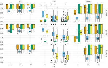
M1: The first 6 vertices are correlated, while the remaining vertices are independent: θ?rs=
● ● ● ● ● ● ● ● ● ● ● ● ● ● ● ● ● ● ● ● ● ● ● ● ● ● ● ● ● ● ● ● ● ● ● ● ● ● ● ● ● ● ● ● ● ● ● ● ● ● ● ● ● ● ● ● ● ● ● ● ● ● ● ● ● ● ●● ● ● ● ● ● ● ● ● ● ● ● ● ● ● ● ● ● ● ● ● ● ● ● ● ● ● ● ● ● ● ● ● ● ● ● ● ● ● ● ● ● ● ● ● ● ● ● ● ● ● ● ● ● ● ● ● ● ● ● ● ● ● ● ● ● ● ● ● ● ● ● ● ● ● ● ● ● ● ● ● ● ● ● ● ● ● ● ● ● ● ● ● ● ● ● ● ● ● ● ● ● ● ● ● ● ● ● ● ● ● ● ● ● ● ● ● ● ● ● ● ● ● ● ● ● ● ● ● ● ● ● ● ● ● ● ● ● ● ● ● ● ● ● ● ● ● ●● ● ● ● ● ● ● ● ● ● ● ● ● ● ● ● ● ● ● ● ● ● ● ● ● ● ● ● ● ● ● ● ● ● ● ● ● ● ● ● ● ● ● ● ● ● ● ● ● ● ● ● ● ● ● ● ● ● ● ● ● ● ● ● ● ● ● ● ● ● ● ● ● ● ● ● ● ● ● ● ● ● ● ● ● ● ● ● ● ● ● ● ● ● ● ● ● ● ● ● ● ● ● ● ● ● ● ● ● ● ● ● ● ● ● ● ● ● ● ● ● ● ● ● ● ● ● ● ● ● ● ● ● ● ● ● ● ● ● ● ● ● ● ● ● ● ● ● ● ● ● ● ● ● ● ● ● ● ● ● ● ● ●
AUC FDR Power
d = 190 d = 1225 d = 4950
20 40 80 20 40 80 20 40 80
0.00 0.25 0.50 0.75 1.00 0.00 0.25 0.50 0.75 1.00 0.00 0.25 0.50 0.75 1.00 n
Method: MCML eLasso Gaussian Pseudolikelihood
Figure 1: The results forM1 model
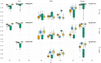
M2: The first 20 vertices have the “chain structure” and the rest are independent: θr?−1,r =
±1 forr ≤20. Again the signs are chosen randomly and the model dimension is 19.
The model M1 corresponds to a dense structure on a small subset of vertices. The model
M2 is a simple structure which involves relatively large subset of vertices.
We consider the following cases: d= 20,50,100. So, the considered number of possible edges (parameters of the model) is ¯d= 190,1225,4950, respectively. For ¯d= 190,1225 we usen= 20,40,80 and for ¯d= 4950 we use n= 40,80.
For each configuration of the model, the number of vertices dand the number of obser-vation n we sample 100 replications of data sets. For sampling a data set we use a final configuration of independent Gibbs samplers of the length 106.
In simulation study we compare our methods to the following methods: the pseudo-likelihood approach, eLassoproposed by van Borkulo et al. (2014) and the Gaussian
ap-proximation from Banerjee et al. (2008). TheeLassomethod is based on separate logistic
models and it is similar to the method proposed by Ravikumar et al. (2010). For all methods excepteLassowe use two stage procedures, which are analogous to Algorithm 1. Namely,
● ● ● ● ● ● ● ● ● ● ● ● ● ● ● ● ● ● ● ● ● ● ● ● ● ● ● ● ● ● ● ● ● ● ● ● ● ● ● ● ● ● ● ● ● ● ● ● ● ● ● ● ● ● ● ●●●●●●●●●●●● ●● ●●●●●●●●●●●●●●●●●●● ● ● ● ● ● ● ● ●● ● ● ● ● ● ● ● ● ● ● ● ● ● ● ● ● ● ● ● ●● ● ● ●●●●●●●●●●●●●●●●●●●●●●●●● ● ● ● ● ● ● ● ●●● ● ●●●●●●●●●●●●●●●● ● ●●●● ● ● ● ● ● ● ● ● ● ● ● ● ● ● ● ● ● ● ● ● ● ● ● ● ● ● ● ● ● ● ● ● ● ● ● ● ● ● ● ● ● ● ● ● ● ● ● ● ● ● ● ● ● ● ● ● ● ● ● ● ● ● ● ● ● ● ● ● ● ● ● ● ● ● ● ● ● ● ● ● ● ● ● ● ● ● ● ● ● ● ● ● ● ● ● ● ● ● ● ● ● ● ● ● ● ● ●●●● ● ● ● ● ● ● ● ● ● ● ● ● ● ● ● ● ● ● ● ● ● ● ● ● ● ● ● ● ● ● ● ● ● ● ● ● ● ●●●●●●●●●●● ●● ●●●●●
AUC FDR Power
d = 190 d = 1225 d = 4950
20 40 80 20 40 80 20 40 80
0.00 0.25 0.50 0.75 1.00 0.00 0.25 0.50 0.75 1.00 0.00 0.25 0.50 0.75 1.00 n
Method: MCML eLasso Gaussian Pseudolikelihood
Figure 2: The results forM2 model
In the comparison we use the following measures of the accuracy. First, to observe the ability of methods to separate true and false edges we compute AUC, where the ROC curve is computed as the threshold δ varies. The estimates are also compared using the false discovery rate (FDR) and the ability of recognizing true edges (denoted by “Power”). The results are summarized in Figure 1 and Figure 2 for modelsM1 andM2,respectively.
In the first model we can observe that our algorithm and the Gaussian approximation work very well and comparably. The latter has slightly larger power, but at the price of slightly larger FDR. The dominance of these two methods over the pseudolikehood estimator and eLassois evident. The pseudolikelihood method finds well true edges, but is not able
to discard false edges. eLassoworks very poorly in this model.
The second model has a simple structure, so both methods based on the pseudolikelihood approach work much better than in M1. The accuracy of the Gaussian approximation is weak in this model. It has substantial problem with finding true edges, especially when
Summarizing, it is difficult to indicate the winner algorithm. We can observe that the quality of our algorithm in selecting the true model is satisfactory. Moreover, only this procedure works on a good level in both models and avoids making noticeable mistakes. The Gaussian approximation works well in M1, but seems to be the weakest in M2. The
eLasso completely fails in M1,but its quality in M2 is high, especially for large sample
sizes. The pseudolikelihood approach in all examples well separates true and false edges, has good power but in comparison with other methods its FDR is too high, so models that it chooses contains many irrelevant edges.
Clearly, by construction the computational cost of our method is larger than its three competitors. However, the whole time that is needed to compute our estimator is reasonable. For instance, for a single data set and n = 40 computing the estimator on 3.4 GHZ CPU takes about 15 seconds for ¯d= 190,60 seconds for ¯d= 1225 and 5 minutes for ¯d= 4950.
Since our algorithm uses only sufficient statistics the dependence on nof its computational cost is negligible. Thus, the computational times forn= 80 are almost the same.
5.2. CAL500 dataset
We apply our method to “CAL500” dataset (Turnbull et al., 2008). Working with a real data set we consider the Ising model (1) with a linear term (an external field). This modification is motivated by the fact that in practice marginal probabilities of Y(s) being +1 or −1 are unknown and should be estimated. The adaptation of our algorithm to this case is straightforward.
For model selection in the Ising model there are no natural measures of the quality of estimates. One would try to compare the prediction ability of obtained estimators, but prediction for the Ising model is challenging itself and results will be biased by the method used to approximate predicted states. Moreover, all considered methods optimize different loss functions, so these loss functions also cannot be used to the honest comparison of the methods. Due to that, we decide to show only the results of our method for the real data example.
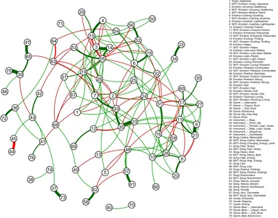
The considered data set consists of 174 binary features and 68 numeric features for 502 songs. We skipped the numeric features and apply our method to find the dependence structure between labels. These labels concerning genre, mood or instrument are annotated to songs. We run our algorithm analogously to the case of simulated data and as the result we obtain a sparse graph with 181 edges, see Figure 3. We observe that founded edges are rather intuitive. For instance, among the most positively correlated labels we have labels de-noted by 3 and 14 (,,Emotion-Arousing-Awakening” and ,,Emotion-Exciting-Thrilling”), 57 and 61 (,,Song-Like” and ,, Song-Recommend”) or 22 and 34 (,,Emotion-Loving-Romantic” and ,,Emotion-Touching-Loving”). On the other hand, the most negatively correlated labels are: 44 and 45 (,,Instrument-Female Lead Vocals” and ,,Instrument - Male Lead Vocals”) or 63 and 64 (,,Song-Texture Acoustic” and ,,Song-Texture Electric”).
6. Conclusions
●
●
●
●
●
●
●
●
●
●
●
●
●
●
●
●
●
●
●
●
●
●
●
●
●
●
●
●
●
●
●
●
●
●
●
●
●
●
●
●
●
●
●
●
●
●
●
●
●
●
●
●
●
●
●
●
●
●
●
●
●
●
●
●
●
●
●
●
●
●
●
●
●
●
●
●
●
●
●
●
●
●
●
●
●
●
●
●
●
●
●
●
●
●
●
●
●
●
●
●
●
●
●
●
●
●
●
●
●
●
●
●
●
●
●
●
●
●
●
●
●
●
●
●
●
●
●
●
●
●
●
●
●
●
●
●
●
●
●
●
●
●
●
●
●
●
●
●
●
●
●
●
1 2 3 4 5 6 7 8 9 10 11 12 13 14 15 16 17 18 19 20 21 22 23 24 25 26 27 28 29 30 31 32 33 34 35 36 37 38 39 40 41 42 43 44 45 46 47 48 49 50 51 52 53 54 55 56 57 58 59 60 61 62 63 64 65 66 67 68 69 70 71 72 73 74 75 76 1: Angry−Agressive 2: NOT−Emotion−Angry−Agressive 3: Emotion−Arousing−Awakening 4: NOT−Emotion−Arousing−Awakening 5: NOT−Emotion−Bizarre−Weird 6: Emotion−Calming−Soothing 7: NOT−Emotion−Calming−Soothing 8: Emotion−Carefree−Lighthearted 9: NOT−Emotion−Carefree−Lighthearted 10: Emotion−Cheerful−Festive 11: NOT−Emotion−Cheerful−Festive 12: Emotion−Emotional−Passionate 13: NOT−Emotion−Emotional−Passionate 14: Emotion−Exciting−Thrilling 15: NOT−Emotion−Exciting−Thrilling 16: Emotion−Happy 17: NOT−Emotion−Happy 18: Emotion−Laid−back−Mellow 19: NOT−Emotion−Laid−back−Mellow 20: Emotion−Light−Playful 21: NOT−Emotion−Light−Playful 22: Emotion−Loving−Romantic 23: NOT−Emotion−Loving−Romantic 24: Emotion−Pleasant−Comfortable 25: NOT−Emotion−Pleasant−Comfortable 26: Emotion−Positive−Optimistic 27: NOT−Emotion−Positive−Optimistic 28: Emotion−Powerful−Strong 29: NOT−Emotion−Powerful−Strong 30: Emotion−Sad 31: NOT−Emotion−Sad 32: Emotion−Tender−Soft 33: NOT−Emotion−Tender−Soft 34: Emotion−Touching−Loving 35: NOT−Emotion−Touching−Loving 36: Genre−−_Alternative 37: Genre−−_Classic_Rock 38: Genre−−_Soft_Rock 39: Genre−Electronica 40: Genre−Hip_Hop−Rap 41: Genre−Rock 42: Instrument_−_Bass 43: Instrument_−_Drum_Set 44: Instrument_−_Female_Lead_Vocals 45: Instrument_−_Male_Lead_Vocals 46: Instrument_−_Sequencer 47: Instrument_−_Synthesizer 48: Song−Catchy−Memorable 49: NOT−Song−Catchy−Memorable 50: NOT−Song−Changing_Energy_Level 51: Song−Fast_Tempo 52: NOT−Song−Fast_Tempo 53: Song−Heavy_Beat 54: NOT−Song−Heavy_Beat 55: Song−High_Energy 56: NOT−Song−High_Energy 57: Song−Like 58: NOT−Song−Like 59: Song−Positive_Feelings 60: NOT−Song−Positive_Feelings 61: Song−Recommend 62: NOT−Song−Recommend 63: Song−Texture_Acoustic 64: Song−Texture_Electric 65: Song−Texture_Synthesized 66: Song−Tonality 67: Song−Very_Danceable 68: NOT−Song−Very_Danceable 69: Vocals−Emotional 70: Vocals−Rapping 71: Vocals−Strong 72: Genre−Best−−_Alternative 73: Genre−Best−−_Classic_Rock 74: Genre−Best−−_Soft_Rock 75: Genre−Best−Electronica 76: Genre−Best−RockFigure 3: The obtained graph for CAL500 dataset. The width of the edges corresponds to the magnitude of|θˆrsδ∗|. The edges with higher absolute value are wider. The color denotes the sign of ˆθrsδ∗: green – positive, red – negative. To improve clarity we do not show edges corresponding to|θˆδ∗
rs|<0.001.
reveals the true dependence structure with high probability. The regularity conditions that we need are not restrictive and are weaker than assumptions used in the other approaches based on the likelihood approximation. Moreover, the theoretical results are completed by numerical experiments. They confirm that the MCMC approximation is able to find the true model in a satisfactory way and its quality is comparable or higher than competing algorithms.
investigating the model (1) with predictors (covariates). The evaluation of the prediction error of the procedure is also a difficult task. Clearly, these problems need detailed studies.
Acknowledgments
We would like to thank the associate editor and reviewers for their comments, that have improved the paper. B la˙zej Miasojedow was supported by the Polish National Science Center grant no. 2015/17/D/ST1/01198. Wojciech Rejchel was supported by the Polish National Science Center grants no. 2014/12/S/ST1/00344 and no. 2015/17/B/ST6/01878.
Appendix A. Auxiliary results
In this section we formulate lemmas that are needed to prove main results of the paper. The roles, that they play, are described in detail at the end of section 3. The first lemma is borrowed from Huang et al. (2013, Lemma 3.1).
Lemma 5 Let θ˜= ˆθ−θ?, z∗ =|∇`mn(θ?)|∞ and
D(ˆθ, θ) = (ˆθ−θ)0h∇`nm(ˆθ)− ∇`mn(θ)i.
Then
(λ−z∗)|θ˜Tc|1 ≤D(ˆθ, θ?) + (λ−z∗)|θ˜Tc|1 ≤(λ+z∗)|θ˜T|1. (20)
Besides, for arbitrary ξ >1 on the event
Ω1 =
|∇`mn(θ?)|∞≤ ξ−1
ξ+ 1λ
(21)
the random vector θ˜belongs to the cone C(ξ, T).
Proof The proof is the same as the proof of Huang et al. (2013, Lemma 3.1). It is quoted here to make the paper complete.
Convexity of the MCMC approximation `mn(θ) easily implies the first inequality in (20). The same property combined with convexity of the Lasso penalty gives us that zero has to belong to the subgradient of (7) at the minimizer ˆθ,i.e.
∇rs`mn(ˆθ) =−λsign(ˆθrs), if ˆθrs6= 0
|∇rs`mn(ˆθ)| ≤λ, if ˆθrs = 0,
(22)
where we use ∇`mn(θ) =
∇rs`mn(ˆθ)
r<s and sign(t) = 1 for t >0, sign(t) =−1 for t <0, sign(t) = 0 fort= 0.Using (22) and properties of the l1-norm we obtain that
D(ˆθ, θ?) = X
(r,s)∈T ˜
θrs∇rs`mn(θ?+ ˜θ) + X
(r,s)∈Tc
ˆ
θrs∇rs`mn(θ?+ ˜θ)−θ˜
0∇`m n(θ?)
≤λ X
(r,s)∈T
|θ˜rs| −λ X
(r,s)∈Tc
|θˆrs|+|θ˜|1z∗
≤λ|θ˜T|1−λ|θ˜Tc|1+z∗|θ˜T|1+z∗|θ˜Tc|1
Thus, the second inequality in (20) is also established. To prove the last claim of the lemma notice that on the event Ω1 we obtain from (20)
|θ˜Tc|1 ≤ λ+z ∗
λ−z∗|θ˜T|1 ≤ξ|θ˜T|1.
The second lemma is an adaptation of Huang et al. (2013, Theorem 3.1) to our problem.
Lemma 6 Let ξ >1. Moreover, let us denoteτ = (ξ+1) ¯d0λ
¯
F(ξ,T) and an event
Ω2 =
τ < e−1 . (23)
Then Ω1∩Ω2⊂A, where A=
|θˆ−θ?|∞≤
2ξeηλ
(ξ+ 1) ¯F(ξ, T)
, (24)
where η <1 is the smaller solution of the equation ηe−η =τ.
Proof Suppose we are on the event Ω1∩Ω2. Denote again ˜θ = ˆθ−θ? and notice that θ= θ˜
|θ˜|1
∈ C(ξ, T) by Lemma 5. Consider the function
g(t) =θ0∇`mn(θ?+tθ)−θ0∇`mn(θ?)
for each t ≥ 0. This function is nondecreasing, because `mn(·) is convex. Thus, we obtain
g(t)≤g(|θ˜|1) for everyt∈(0,|θ˜|1). On the event Ω1 and from Lemma 5 we have that θ0[∇`mn(θ?+tθ)− ∇`mn(θ?)] + 2λ
ξ+ 1|θTc|1≤ 2λξ
ξ+ 1|θT|1. (25) In further argumentation we consider all nonnegative t satisfying (25), that is an interval [0,˜t] for some ˜t >0. Proceeding similarly to the proof of Huang et al. (2013, Lemma 3.2) we obtain
tθ0[∇`mn(θ?+tθ)− ∇`mn(θ?)]≥t2exp(−γtθ)θ0∇2`mn(θ?)θ , (26) whereγtθ=tmaxk,l|θ0J(Yk)−θ0J(Yl)| ≤2t,becauseJ(Yk) = Yk(r)Yk(s)
rsand|θ|1 = 1. Therefore, the right-hand side in (26) can be lower bounded by
t2exp(−2t)θ0∇2`mn(θ?)θ . (27) Using the definition of ¯F(ξ, T),the fact thatθ∈ C(ξ, T),the bound (27) and (25) we obtain
texp(−2t)F¯(ξ, T)|θT|
2 1
¯
d0 ≤texp(−2t)θ 0∇2`m
n(θ?)θ
≤θ0[∇`mn(θ?+tθ)− ∇`mn(θ?)]
≤ 2λξ
ξ+ 1|θT|1− 2λ ξ+ 1|θTc|1
So, every t satisfying (25) has to fulfill the inequality 2texp(−2t) ≤ τ. In particular, 2˜texp(−2˜t)≤τ.We are on Ω2,so it implies that 2˜t≤η,where η is the smaller solution of the equationηexp(−η) =τ. We know also that|θ˜|1 ≤˜t, so
|θ˜|1exp(−η)≤˜texp(−2˜t)≤ ˜texp(−2˜t)θ 0∇2`m
n(θ?)θ ¯
F(ξ, T)|θT|1|θ|∞ ≤ θ
0
∇`mn(θ?+ ˜tθ)− ∇`mn(θ?) ¯
F(ξ, T)|θT|1|θ|∞
≤ 2λξ
(ξ+ 1) ¯F(ξ, T)|θ|∞ ,
where we have used bounds (27) and (25). Using the equality |θ|∞ = | ˜
θ|∞
|θ˜|1, we finish the proof.
Lemma 7 For every natural n, m and positivet P(|∇`mn(θ?)|∞≤t)≥1−2 ¯dexp −nt2/8−β1exp
−mβ2
4M2
−2 ¯dβ1exp
−t 2mβ2
64M2
.
Proof We can rewrite ∇`mn(θ?) as
∇`mn(θ?) =−
" 1
n
n X
i=1
J(Yi)−
∇C(θ?)
C(θ?) #
+
1
m m P
k=1 wk(θ?)
h
J(Yk)−∇CC(θ(θ??))
i
1
m m P
k=1 wk(θ?)
(28)
Notice that the first therm in (28) depends only on the initial sampleY1, . . . , Yn and is an average of i.i.d random variables. The second term depends only on the MCMC sample
Y1, . . . , Ym. We start the analysis with the former one. Using Hoeffding’s inequality we obtain for each naturaln, positivet and a pair of indicesr < s
P
1
n
n X
i=1
Jrs(Yi)−
∇rsC(θ?)
C(θ?)
> t/2 !
≤2 exp −nt2/8.
Therefore, by the union bound we have
P
1
n
n X
i=1
J(Yi)−
∇C(θ?)
C(θ?)
∞ > t/2
!
≤2 ¯dexp −nt2/8
. (29)
Next, we investigate the second expression in (28). Its denominator is an average that depends on the Markov chain. To handle it we can use Theorem 4 in section 3. Notice that
exp[(θ?)0J(y)]
h(y) ≤M C(θ
?) for everyyand
EY∼hexp[(θ
?)0J(Y)]
h(Y) =C(θ
?).Therefore, for everyn, m
P 1 m
m X
k=1
wk(θ?)≥C(θ?)/2 !
≥1−β1exp
−mβ2
4M2
Finally, we bound the l∞-norm of the numerator of the second term in (28). We fix a pair of indicesr < s. It is not difficult to calculate that
EY∼h
exp [(θ?)0J(Y)]
h(Y)
Jrs(Y)−
∇rsC(θ?)
C(θ?)
= 0
and for everyy
exp((θ?)0J(y) h(y)
Jrs(y)−
∇rsC(θ?)
C(θ?)
≤2M C(θ?).
From Theorem 4 we obtain for every positive t
1
m
m X
k=1 wk(θ?)
Jrs(Yk)−
∇rsC(θ?)
C(θ?)
≥tC(θ?)/4
with probability at least 1−2β1exp
−t2mβ2
64M2
. Using union bounds we estimate the
nu-merator of the second expression in (28). This fact and (30) imply that for every positivet
and naturaln, mwith probability at least 1−β1exp
−mβ2
4M2
−2 ¯dβ1exp
−t2mβ2
64M2
we have
1
m m P
k=1 wk(θ?)
h
J(Yk)−∇CC(θ(θ??))
i
1
m m P
k=1 wk(θ?)
∞
≤t/2. (31)
Taking (29) and (31) together we finish the proof.
Corollary 8 Let ε >0, ξ >1 and
λ= ξ+ 1
ξ−1max
2 r
2 log(2 ¯d/ε)
n ,8M
s
log(2 ¯d+ 1)β1/ε mβ2
.
Conditions (13) and (14) imply
P(Ω1)≥1−2ε . Proof We take t= ξξ−1+1λin Lemma 7.
Lemma 9 For every n, m and positive t P ∇2`mn(θ?)− ∇2logC(θ?)
∞≤t
≥ 1−2β1exp
−mβ2
4M2
− 2 ¯d( ¯d+ 1)β1exp
−t 2mβ2
256M2
Proof To estimate thel∞-norm of the matrix difference in (32) we boundl∞-norms of two matrices:
m P
k=1
wk(θ?)J(Yk)⊗2
m P
k=1 wk(θ?)
−∇ 2C(θ?)
C(θ?) =
1
m m P
k=1 wk(θ?)
h
J(Yk)⊗2−∇C2C(θ(?θ)?)
i 1 m m P k=1 wk(θ?)
(33) and 1 m m P k=1
wk(θ)J(Yk)
1
m m P
k=1 wk(θ)
⊗2 − ∇
C(θ?)
C(θ?) ⊗2
. (34)
The denominator of the right-hand side of (33) has been estimated in the proof of Lemma 7, so we bound the numerator. We can calculate that
EY∼h
exp [(θ?)0J(Y)]
h(Y)
J(Y)⊗2−∇ 2C(θ?)
C(θ?)
= 0
and for everyy and two pairs of indicesr < s, r0 < s0 we have
exp((θ?)0J(y)
h(y)
Jrs(y)Jr0s0(y)−
∇2
rs,r0s0C(θ?)
C(θ?)
≤2M C(θ?).
Using the union bound and (30) we upper-bound thel∞-norm of the right-hand side of (33) by t/2 with probability at least
1−β1exp
−mβ2
4M2
−2 ¯d2β1exp
−t 2mβ
2
64M2
.
The last step of the proof is handling with the l∞-norm of (34). This expression can be upper-bounded by m P k=1
wk(θ)J(Yk)
m P
k=1 wk(θ)
−∇C(θ
?)
C(θ?) ∞ m P k=1
wk(θ)J(Yk)
m P
k=1 wk(θ)
∞ +
∇C(θ?)
C(θ?) ∞ ∞ . (35)
The first term in (35) has been bounded with high probability in the proof of Lemma 7. The remaining two can be easily estimated by one. Therefore, for every positivet thel∞-norm of (34) is not greater than t/2 with probability at least
1−β1exp
−mβ2
4M2
−2 ¯dβ1exp
−t 2mβ2
256M2
.
Corollary 10 If (14), then for every ε >0 the following inequality
¯
F(ξ, T)≥F(ξ, T)−16 ¯d0(1 +ξ)2M
s log
2 ¯d( ¯d+ 1)β1/ε
mβ2
has probability at least 1−2ε. Proof We take
t= 16M
s
log2 ¯d( ¯d+ 1)β1/ε mβ2
in Lemma 9 and use Huang et al. (2013, Lemma 4.1 (ii)).
Appendix B. Proofs of main results
Proof [Proof of Theorem 2] Fix ε >0, ξ >1 and denote γ =γ(ξ) = αα(ξ()−2ξ) ∈(0,1).First, from Corollary 8 we know thatP(Ω1)≥1−2ε.Using the condition (14) we obtain that
F(ξ, T)−16 ¯d0(1 +ξ)2M
s log
2 ¯d( ¯d+ 1)β1/ε
mβ2
≥γF(ξ, T).
Therefore, from Corollary 10 we have thatP( ¯F(ξ, T)≥γF(ξ, T))≥1−2ε.It is not difficult to calculate that
(1 +ξ) ¯d0λ γF(ξ, T) ≤e
−1,
so we have also P(Ω2) ≥ 1−2ε. To finish the proof we use Lemma 6 (with η = 1 for
simplicity) and again bound ¯F(ξ, T) from below byγF(ξ, T) in the eventAdefined in (24).
Proof [Proof of Corollary 3] The proof is a simple consequence of the uniform bound (15) obtained in Theorem 2. Indeed, for an arbitrary pair of indices (r, s)∈/T we obtain
|θˆrs|=|θˆrs−θ?rs| ≤Rmn ,
so (r, s)∈/ T .ˆ Analogously, if we take a pair (r, s)∈T, then
References
Yves F. Atchad´e, Gersende Fort, and Eric Moulines. On perturbed proximal gradient algorithms. Journal of Machine Learning Research, 18:310–342, 2017.
Onureena Banerjee, Laurent El Ghaoui, and Alexandre d’Aspremont. Model selection through sparse maximum likelihood estimation for multivariate gaussian or binary data.
Journal of Machine Learning Research, 9:485–516, 2008.
Amir Beck and Marc Teboulle. A fast iterative shrinkage-thresholding algorithm for linear inverse problems. SIAM Journal on Imaging Sciences, 2:183–202, 2009.
Julian Besag. Spacial interaction and the statistical analysis of lattice systems. Journal of the Royal Statistical Society, Series B, 36:192–236, 1974.
Peter J Bickel, Ya’acov Ritov, and Alexandre B Tsybakov. Simultaneous analysis of Lasso and Dantzig selector. The Annals of Statistics, 37:1705–1732, 2009.
Guy Bresler, Elchanan Mossel, and Allan Sly. Reconstruction of Markov random fields from samples: Some observations and algorithms. InApproximation, Randomization and Combinatorial Optimization. Algorithms and Techniques, pages 343–356. Springer, 2008. Peter B¨uhlmann and Sara van de Geer. Statistics for high-dimensional data: methods,
theory and applications. Springer Series in Statistics, New York: Springer, 2011.
Jianqing Fan and Runze Li. Variable selection via nonconcave penalized likelihood and its oracle properties. Journal of the American Statistical Association, 96:1348–1360, 2001. Charles J Geyer. On the convergence of Monte Carlo maximum likelihood calculations.
Journal of the Royal Statistical Society. Series B (Methodological), 56:261–274, 1994. Charles J Geyer and Elizabeth A Thompson. Constrained Monte Carlo maximum likelihood
for dependent data. Journal of the Royal Statistical Society. Series B (Methodological), 54:657–699, 1992.
Jian Guo, Elizaveta Levina, George Michailidis, and Ji Zhu. Joint structure estimation for categorical Markov networks. Technical report, 2010.
Holger H¨ofling and Robert Tibshirani. Estimation of sparse binary pairwise Markov net-works using pseudolikelihoods. Journal of Machine Learning Research, 10:883–906, 2009. Jean Honorio. Convergence Rates of Biased Stochastic Optimization for Learning Sparse Ising Models. InProceedings of the 29th International Conference on Machine Learning, pages 1099–1106, 2012.
Jian Huang and Cun-Hui Zhang. Estimation and selection via absolute penalized convex minimization and its multistage adaptive applications. Journal of Machine Learning Research, 13:1839–1864, 2012.
Ernst Ising. Beitrag zur theorie des ferromagnetismus. Zeitschrift f¨ur Physik A Hadrons and Nuclei, 31(1):253–258, 1925.
Ali Jalali, Christopher C Johnson, and Pradeep K Ravikumar. On learning discrete graphi-cal models using greedy methods. InAdvances in Neural Information Processing Systems, pages 1935–1943, 2011.
Ioannis Kontoyiannis and Sean P Meyn. Geometric ergodicity and the spectral gap of non-reversible markov chains. Probability Theory and Related Fields, 154:327–339, 2012. Su-In Lee, Varun Ganapathi, and Daphne Koller. Efficient Structure Learning of Markov Networks usingl1-Regularization. InAdvances in Neural Information Processing Systems,
pages 817–824, 2006.
B la˙zej Miasojedow. Hoeffding’s inequalities for geometrically ergodic markov chains on general state space. Statistics & Probability Letters, 87:115–120, 2014.
Elchanan Mossel and Allan Sly. Exact thresholds for Ising–Gibbs samplers on general graphs. The Annals of Probability, 41:294–328, 2013.
Sahand Negahban, Bin Yu, Martin J Wainwright, and Pradeep K Ravikumar. A unified framework for high-dimensional analysis ofM-estimators with decomposable regularizers. In Advances in Neural Information Processing Systems, pages 1348–1356, 2009.
Piotr Pokarowski and Jan Mielniczuk. Combined l1 and greedy l0 penalized least squares for linear model selection. Journal of Machine Learning Research, 16:961–992, 2015. Pradeep Ravikumar, Martin J Wainwright, and John Lafferty. High-dimensional Ising model
selection using l1-regularized logistic regression. The Annals of Statistics, 38:1287–1319, 2010.
Gareth O Roberts and Jeffrey S Rosenthal. Geometric ergodicity and hybrid Markov chains.
Electronic Communications in Probability, 2:13–25, 1997.
Robert Tibshirani. Regression shrinkage and selection via the lasso. Journal of the Royal Statistical Society. Series B (Methodological), 58:267–288, 1996.
Douglas Turnbull, Luke Barrington, David Torres, and Gert Lanckriet. Semantic annotation and retrieval of music and sound effects. IEEE Transactions on Audio, Speech, and Language Processing, 16:467–476, 2008.
Claudia D. van Borkulo, Denny Borsboom, Sacha Epskamp, Tessa F. Blanken, Lynn Boschloo, Robert A. Schoevers, and Lourens J. Waldorp. A new method for constructing networks from binary data. Scientific Reports, 4, 2014.
Sara van de Geer. High-dimensional generalized linear models and the lasso. The Annals of Statistics, 36:614–645, 2008.
Martin J. Wainwright and Michael I. Jordan. Log-determinant relaxation for approximate inference in discrete markov random fields. IEEE Transactions on Signal Processing, 54: 2099–2109, 2006.
Lingzhou Xue, Hui Zou, and Tianxi Cai. Nonconcave penalized composite conditional likelihood estimation of sparse Ising models. The Annals of Statistics, 40:1403–1429, 2012.
Fei Ye and Cun-Hui Zhang. Rate Minimaxity of the Lasso and Dantzig Selector for thelq loss in lr Balls. Journal of Machine Learning Research, 11:3519–3540, 2010.
Tong Zhang. On the consistency of feature selection using greedy least squares regression.
Journal of Machine Learning Research, 10:555–568, 2009.
Peng Zhao and Bin Yu. On model selection consistency of Lasso. Journal of Machine Learning Research, 7:2541–2563, 2006.