Application to Differential Transformation Method for Solving Eight Order Ordinary Differential Equations

ISSN: 2231-5373

http://www.ijmttjournal.org

Page 177

Application to Differential Transformation

Method for Solving Eight Order Ordinary

Differential Equations

1

Prof. Narhari Onkar Warade, 2Dr. Prabha Rastogi

1

Research Scholar Dept. of Mathematics, J.J.T. University Churu, Rajasthan, India 2

Dept. of Mathematics, J.J.T. University Churu, Rajasthan, India

Abstract

The Zhou's differential transform method (ZDTM) is approximate method which construct analytical solution in the firm of polynomial which can be easily applied o many linear and non linear problems by reducing lot of computational work as compare to Tayler series for higher order linear differential equations initial value problems. In this paper the definition and operation of the one dimensional Zhou's differential transform method and investigate the particular exact solutions of eight order ordinary differential equations initial value problems by explaining concept of ZDTM obtain solution of three numerical examples for demonstration. the results are compared with exact solution with graphs. It is observed that solutions obtained from this ZDTM technique have very high degree of accuracy.

There results show that the technique introduced here is accurate & easy to apply.

Keywords :- Ordinary differential equitations zhou’s Method (DTM), Initial value problem

I. INTRODUCTION

The Zhou's differential transformation method is a numerical method based on a Taylor expansion method beyond the treatment of ODE'S with the ZDTM in which case one should at least clearly refer to the numerous studies done with the Taylor series mehtod. It seems that the major contribution of the ZDTM is in the easy generalization of the Taylor method.

Biazar J. et al used ZDTM for Solving quadratic Riccati differential equation [1], Opanuga Used for solving numerical solution of systems of ordinary differential equation by numerical analytical method [2], Chen C. K. and S. S. Chen used ZDTM to obtained the solution of nonlinear system of differential equations [3], Zhou X. Applied ZDTM for Electrical Circuits problems [4], Ayaz F. used ZDTM to find series solution of system of differential equations [5], Duan Y.R. Liu used ZDTM for Burger's equation to obtain series solutions [6], Bert W. has applied DTM on system of linear equation and analysis of its solutions[7], Chen C.L. has applied DTM technique for steady nonlinear beat conduction problems[8], Using DTM Hassan have find out series solution and that solution compared with DTM method for linear & non linear initial value problems & proved that DTM is reliable tool to find numerical solution[9], Khaled Batiha has been used DTM to obtain the Taylor’s series as solution of linear, nonlinear system of ordinary differential equations[10], Montri Thangmoon has been used to find numerical solution of ordinary differential equations[11], Edeki, A semi method for solutions of a certain class of second order ordinary differential equations [12], Gbadeyan and Agboola for Dynamic behaviour of a double Rayleigh beam-system due to uniform AriKoglu A applied DTM to obtain numerical solution of differential equations partially distributed moving load [13] Abdel Halim Hassan I. used DTM method for solving differential equations[14] Arikoglu A applied DTM to obtained numerical solution of differential equation [15], Kou B has been used to find numerical solution of the free convection problems[16].

II. BASICDEFINITIONS&PROPERTIESOFDTMMETHOD

v(t) can be expressed by Taylor’s series, then v(t) can be represented as v(t) =

∞ Σ k = 0

(t−ti)k k! V(k)

ISSN: 2231-5373

http://www.ijmttjournal.org

Page 178

∴ v(t) =

∞ Σ k = 0

(t−ti)k

k! V(k) = D-1 V(k)

v (t)=

∞ Σ k = 0

(t−ti)k

k! V(k) + R n +1 (t)

by Taylor’s Series

V (k) = _k!1 dk_dtv(t)_k at t = t0

III. FUNDAMENTALTHEOREMSONDTM

Theorem 1 :- If n (t) = p(t) + s(t) then N(k) = P (k) + S(k) Theorem 2 :- If n(t) = ∝ (t) then ∝ p (t) then

N (k) = ∝ P(k) Theorem 3 :- If n (t) = dp (t)_dt then

N (k) = (k+1) P (k+1) Theorem 4 :- If n (t) = d2_dtp (t)₂ then

N (k) = (k+1) (k+2) (k+2) P (k+2) Theorem 5 :- If n (t) = dn_dtp (t)_n then

N (k)= (k+1) (k+2) (k+3)… (k+n) P (K+n) Theorem6 :- If n(t) = tn them

N(K) =

k Σ

l = 0S(l) P(k-l)

Theorem7 :- If n (t) = tn them

N(k) = δ (k-n)

δ (k-n) = 1 if k = n_{0 if k ≠ n} Theorem 8:- If n (t) = eλt then

N (k) = λ_k!k Theorem 9:- If n(t) = (1+t)n then

N(k) = M n−1 ..(n−k+1)_k! Theorem 10:- if n(t) = (1+t)n then

N(k) = w_kiksin (πk₂ +∝) Theorem 11:- if n(t) = cos (wt +∝) then

N(k)= w_kik cos (πk₂ +∝) Theorem 12 :- if P(k) = D[p(t)]

S(k) = D[s(t)]’ & C1, C2 Are independent of t, k then

ISSN: 2231-5373

http://www.ijmttjournal.org

Page 179

ISSN: 2231-5373

http://www.ijmttjournal.org

Page 180

V. EXPERIMENTATIONOFZDTMRESULTS

Example : 1

Solve non homogeneous linear differential equation yviii – yiv=0

y(0) = yi(0) = yii (0) = 0, yiii (0)=78, yiv(0) = 0, yv(0) = 0, yvi (0) = 0 yvii (0) = 78,

→ Exact Solution is

Y = 78 sinhx – 78 sinx 13x3

By DTM

(k+1) (k+2) (k+3) (k+4) (k+5) (k+6) (k+7) (k+8) U (k+8) = (k+1) (k+2) (k+3) (k+4) U (k+4)

Put k = 0, 1, 2, 3, 4, 5…… U (0) = 0 U (1) = 0

U (2) = 0 U (3) = 78 U (4) = 0 U (5) = 0 U (6) = 13 U (7) = ₁₄₀13 U (8) = 0 U (9) = 0 U (10) = 0 U (11) = 0 U (12) = 0 U (13) = 0 U (14) = 0 U (15) = 0 U (16) = 0

u (+) = 78t3 + ₁₄₀13 t3 + ₁₄₀13 x_8.9.10.111 t13 + (_{8.9.10.11.12.13.14.15} 13 x₁₄₀1 ) t15 +….

Table 1 : Numerical Result for example 2

t Exact D.T.M. DTM Error

0 0.00000 0.00000 0.00000

0.2 0.104000 0.104000 0.00000

0.4 0.832050 0.832050 0.00000

0.6 2.808866 2.808866 0.00000

0.8 6.662491 6.662491 0.00000

ISSN: 2231-5373

http://www.ijmttjournal.org

Page 181

Example 2 Numerical Examples :-

y viii – y vi = 2sin x Boundary conditions y(0) = yi (0) = yii (0) = yiii (0) = 0

yiv (0) = 0, yv (0) = 2, yvi (0) = 0, yvii (0) = 0

Exact soin is given my

y = -2x + sinhx + sinx

(K+1) (K+2) (K+3) (K+4) (K+5) (K+6) (K+7) (K+8) U(8) – (k +1) (k+2) (k+3) (k+4) U (6) 2 (1)_𝑘1𝑘 sin (𝜋𝑘₂)

Put K = 0, 1, 2, 3, 4, 5, 6……

8! U (8) – 6! U(6) = 2 (1)_0!0 sin0 8! U (8) = 6! U(6) = 0

= 6! x 2 U(8) = ₂₈1

K=1 2,3,4,5,6,7,8,9 U(9) – 7! U(7) = 2 9! U (9) = 2

U(9) = _9!2

K=2 3,4,5,6,7,8,9,10, U(10) - 3,4,5,6,7,8 U(8) = 0 7,8,9,10, U(10) = 3,4,5,6, 2 x 1

= 2

0

2

4

6

8

10

12

14

0

0.2

0.4

0.6

0.8

1

ISSN: 2231-5373

http://www.ijmttjournal.org

Page 182

U(10) = _8.9.102 = _4x9x1012 = ₃₆₀1

K=3 4, 5, 6, 7, 8, 9, 10, 11 U(11) – 4,5,6,7,8,9, U(9) = −2_3! – 1₃ = – 1₃

4, 5, 6, 7, 8, 9, 10, 11 U(11) = 0 U (11) = 0

K=4 5, 6, 7, 8, 9, 10, 11, 12 U(12) – 5,6,7,8,9,10 U(10) = 0 5, 6, 7, 8, 9, 10, 11, 12 U(12) – 5,6,7,8,9,10 U(10) = 0

U(12) – _6,8,9,10,111

u(+)= U(0) + tU(1) + t2U(2) + t3U(3) + t4U(4) + t5U(5) + t6U(6) + t7U(7) + t8U(8) + t9U(9) + t10U(10) + t11U(11) + t12U(12) + ……….

= _5!2 t5 + ₂₈1 t8 + _9!2 t9 + ₃₆₀1 t10 + _6,8,9,10,111 + t12 + …..

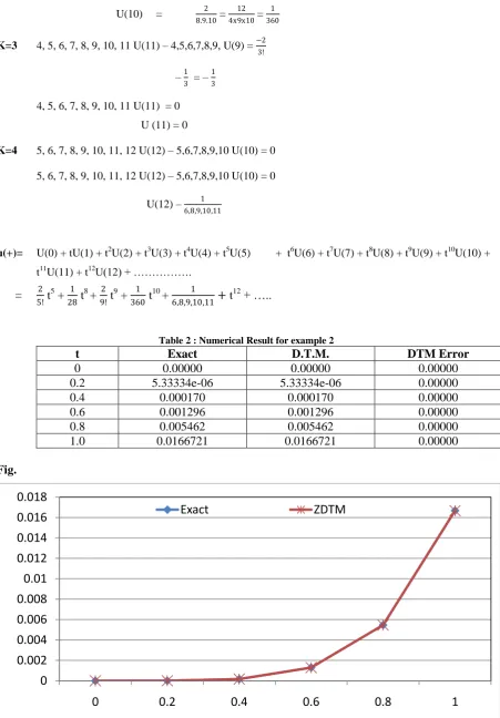
Table 2 : Numerical Result for example 2

t Exact D.T.M. DTM Error

0 0.00000 0.00000 0.00000

0.2 5.33334e-06 5.33334e-06 0.00000

0.4 0.000170 0.000170 0.00000

0.6 0.001296 0.001296 0.00000

0.8 0.005462 0.005462 0.00000

1.0 0.0166721 0.0166721 0.00000

Fig.

0

0.002

0.004

0.006

0.008

0.01

0.012

0.014

0.016

0.018

0

0.2

0.4

0.6

0.8

1

ISSN: 2231-5373

http://www.ijmttjournal.org

Page 183

yiv + y11 = 2 sin hx y(0) = y1(0) = yII(0) yIII(0), yIV(0) = 0 yv(0) = ₅₁2, yvi (0)= 0, yvii(0) = 0

Extract Solution is

y = sinx + sinhx – 2x By DTM

(K+1) (K+2) (K+3) (K+4) (K+5) (K+6) (K+7) (K+8) U (K+8) + (K+1) (K+2) (K+3) (K+4) U (K+4)

= (1)_𝑘!𝑘+(−1)_𝑘!𝑘

Put k = 0 8! U(8) + 4! U (4) = 2 U(8) = _8!2 K= 1 9! U(9) + s! U(5) = 0

9! U(9) = – 5! U(9) = −5! x 2_9!

= _9x8x7x3−1 = -1

K=2 3,4,5,6,7,8,9,10, U(10) + 3,4,5,6, U(6) =1 0 U(10) = _{34,5,6,7,8,9,10}1 K=3 4,5,6,7,8,9,10,11 U(11) + 4,5,6,7U(7)₀ =0

U(11) =0

K= 4 5,6,7,8,9,10,11 U(12) + 5,6,7,8, x _8!2 = _4!2 5, 6,7,8,9,10,11,12 U(12) + 5,6,7,8 x _8!2 x _4!2 5,6,7,8,9,10,11,12 (12) + _4!2

= ₁₂1 - ₁₂1 = 0 U (12) = 0

K = 5 6,7,8,9,10,11,12,13U (13) + 6,7,8,9U (9) = 0

∴ 6,7,8,9,10,11,12,13 U(13) + 2 x -1 =0 6,7,8,9,10,11,12,13 U(13) = 2

ISSN: 2231-5373

http://www.ijmttjournal.org

Page 184

K=6 7,8,9,10,11,12,13,14 U(14) + 7,8,9,10 U(10) = _6!2 7,8,9,10,11,12,13,14 U (14) x _3,5,6,7,1 = _6!2 = _6x5x4x31 U (14) = 0

U= U(0) + U(1)t + U(2) t2 + U(3) t3 + U(W) t4 + U(5) t5 + U(6) t6 + U(7) t7 + U(8)t8 + U(12) t12 + U(13) t13 + U(14) t14

U= 0 + _5!2 t5 + _8!2 t8 + (_9x8x7x3−1 ) t9 + _{3,4,5,6,7,8,9,10}1 t10 + U + 0 + _{6,7,8,9,10,11,12,13}2 t3 + 0 + ……

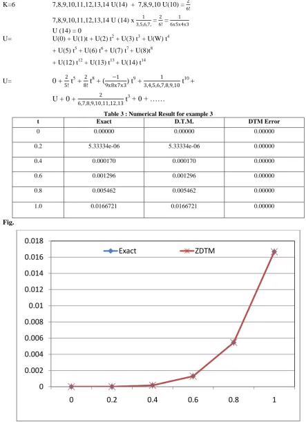
Table 3 : Numerical Result for example 3

t Exact D.T.M. DTM Error

0 0.00000 0.00000 0.00000

0.2 5.33334e-06 5.33334e-06 0.00000

0.4 0.000170 0.000170 0.00000

0.6 0.001296 0.001296 0.00000

0.8 0.005462 0.005462 0.00000

1.0 0.0166721 0.0166721 0.00000

Fig.

VI. VALIDATIONANDCOMPARISON

The ZDTM has promissing approach for many application in various field of science. The drawback of ZDTM is solution is truncated series which does not exhibit the behavious of given problem but gives good approximation or turn solution in small region multistep ZDTM accelerates accuracy of ZDTM The fact is ZDTM is applicable to many other nonlinear models which is reliable than existing other methods.

0

0.002

0.004

0.006

0.008

0.01

0.012

0.014

0.016

0.018

0

0.2

0.4

0.6

0.8

1

ISSN: 2231-5373

http://www.ijmttjournal.org

Page 185

In this work ZDTM applied for initial value problems of ordinary differential equation for eight order ordinary differential equations it reduces the computational difficulties of other traditional methods like Laplase Trans method, Exact solutions by complimentary functions and particular integral method etc. ZDTM is reliable method that needs less work and dose not require any kind of strong assumptions by increasing the order of approximate more accuracy can be obtained graphical comparison show that ZDTM is powerful method.

REFERENCES

[1] Biazar, J., and Eslami, M., 2010, “Differential transform method for quadratic Riccati differential equations,” International Journal of Nonlinear Science, 9(4),pp. 444-447.

[2] Opanuga, A. A. Edeki, S.O., Okagbue, H. I. Akinloabi, G. O., Osheku, A. S. and Ajayi, B., 2014, “On numerical solutions of system of ordinary differential equations by numerical-analytical method,” Applied Mathematical Sciences. 8, pp. 8199-8207. doi.org/10-12988/ams.2014-410807.

[3] Chen C. K. and S.S. Chen, Application of the differential transform method to a non-linear conservative system, applied Mathematics and computation, 154, 431-441 (2004)

[4] Zhou X., Differential Transformation and its Applications for Electrical Circuits, Huazhong University Press, Wuhan, China, 1986 (in Chinese)

[5] Anyaz F., Solutions of the system of differential equations by differential transform method. Applied Mathematics and Computation, 147, 547-567 (2004).

[6] Duan Y., R. Liu and Y. Jaing, Lattice Boltzmann model for the modified Burger’s equation, Appl. Math. Computer, 202, 489-497 (2008)

[7] Bert. W. H. Zeng, Analysis of axial vibration of compound bars by differential transform method. Journal of Sound and Vibration, 275, 641-647 (2004)

[8] Chen C.L. and Y.C. Liu. Differential transformation technique for steady nonlinear heat conduction problems, Appl. Math. Computer, 95, 155164 (1998)

[9] Hassanl H. Abdel-Halim Comparison differential transformation technique with Admain decomposition method for linear and nonlinear initial value problems, Choas Solution Fractals, 36(I) , 53-65 (2008)

[10] Khaled Batiha and Belal Batiha, A New Algorithm for Solving Lnear Ordinary Differential Equations, World Applied Sciences Journal, 15(12), 1774-1779, (2011), ISSN 1818-4952, IDOSI Publications.

[11] Montri Thongmoon, Sasitorn Pusjuso The numerical solutions of differential transform method and the Laplace transforms method for a system of differential equations, Nonlinear Analysis: Hybrid System, 4 425-431 (2010)

[12] Edeki, S.O., Okaghue, Opanuga, A. A., and S. A. Adeosun, 2014, “A semi-analytical method for solutions of a certain class of second order ordinary differential equations” Applied mathematics, 5, pp. 2034-2041 doi.org/10.4236/am.2014-513196

[13] Gbadeyan, J. A., and Agboola, O.O., 2012, “Dynamic behaviour of a double Rayleigh beam-system due to uniform partially distributed moving load,” Journal of Applied Sciences Research, 8(1), pp. 571-581.

[14] Abdel-Halim Hassan I.H., differential transform technique for solving higher order initial value problems, Applied Mathematics and Computation, 154, 299-311 (2004)

[15] Arikoglu A. and Ozkol I., Solution of difference equations by using differential transform method. Pplied Mathematics and Computation 174, 1216-1228 (2006)