Research Journal
Volume 10, No. 30, June 2016, pages 9–18
DOI: 10.12913/22998624/62826 Research Article
EEULA: AN ENERGY-AWARE EVENT-DRIVEN UNICAST ALGORITHM
FOR WIRELESS SENSOR NETWORK BY LEARNING AUTOMATA
Ali Azimi Sotudeh Kashani1, Ali Mohamad Monjezi Noori1
1 Departments of Computer, Shoushtar Branch, Islamic Azad University, Shoushtar, Iran, e-mail: azimi.kashani@
gmail.com
ABSTRACT
Energy consumption is one of the major challenges in wireless sensor networks, thus necessitating an approach for its minimization and for load balancing data. The net-work lifetime ends with the death of one of its nodes, which, in turn, causes energy depletion in and partition of the network. Furthermore, the total energy consumption of nodes depends on their location; that is, because of the loaded data, energy dis-charge in the nodes close to the base station occurs faster than other nodes, the model presented here, through using learning automata, selects the path appropriate for data transferring; the selected path is rewarded or penalized taking the reaction of sur-rounding paths into account. We have used learning automata for energy management
in finding the path; the routing protocol was simulated by NS2 simulator; the lifetime,
energy consumption and balance in an event-driven network in our proposed method were compared with other algorithms.
Keywords: network lifetime; wireless sensor network; learning automata; energy
ef-ficiency algorithm.
INTRODUCTION
A wireless sensor network is made up of many randomly distributed sensor nodes, gather-ing information from the environment, process-ing and sendprocess-ing them to the base station. Sensor networks have vital scientific, medical, econom-ic and military appleconom-ications. These sensor nodes have limited energy, computational capacity, and memory [1]. Generally, each sensor node includes three main subsystems: i) to collect data from environment, ii) to process collected data inside each node, and iii) to exchange data. For each node, a power source, like a battery, is also needed, which is sometimes impossible and sometimes undesired to be recharged, as the sensor may not be accessible in some locations. On the other hand, the network must have long enough lifetime to fulfill its task; hence, having sufficient energy in each node is of vital signifi-cance [2].
Because of its importance in sensor networks, energy has to be wisely managed to extend the lifetime of the sensor nodes during their mission. Energy can be wasted through: i) idle listening; that is, listening to an idle channel in order to receive possible traffic, ii) collision, the situation a node receives more than one packet at the same time, iii) overhearing, meaning a node receives packets destined to other nodes, iv) investigat-ing the control-packet overhead; indeed, a mini-mal number of control packets should be used to make a data transmission, and v) over-emitting, caused by the transmission of a message when the destination node is not ready. On the other hand, transmitting some data consumes much more energy than processing the same data; for instance, with the energy consumed for transmit-ting one bit of information, one thousand bits of information can be processed. Therefore, energy management and saving in a wireless sensor net-work is essential.
Generally, energy-aware protocols are either i) designed to decrease the total energy consump-tion of the network, or ii) to manage available energy to prevent network partitioning, and thus, balance energy consumption [4]. Our proposed algorithm can both manage and save energy. It has been shown that learning automata is a very convenient tool to use in sensor networks, be-cause of its features, such as low computational overhead, ability to use in distributed environ-ments with inaccurate information, and adapta-tion to environmental changes [5-6].
This algorithm is compared to energy aware routing (EAR), directed diffusion, the geodesic sensor clustering protocol (GESC), and energy-efficient and collision-aware multipath routing protocol (EECA) and it has been shown that our algorithm is better than other algorithms.
LITERATURE REVIEW
The existing routing protocols in sensor networks can be classified into proactive/table-driven and reactive/on-demand routing proto-cols [7]. Proactive routing protoproto-cols try to con-tinuously evaluate the routes within the network, so that when a packet needs to be forwarded, the route is already known and can be immediately used. Reactive protocols invoke a route deter-mination procedure on an on-demand basis. The reactive route discovery is usually based on a query-reply exchange, where the route query is flooding through the network to reach the de-sired destination [8-9]. An approach for a better trade-off between proactive and reactive routing is to make use of hybrid routing protocols [10], being both proactive and reactive in their nature. Several route finding algorithms have been de-veloped so far, including hierarchy-, location-, and QoS-based, and data-oriented protocols [11]. In this paper, we compare our algorithm to energy aware routing (EAR), directed diffusion, the geodesic sensor clustering protocol (GESC) [14], and energy-efficient and collision-aware multipath routing protocol (EECA)[15].
The EAR, an important energy-aware rout-ing protocol in sensor networks, uses floodrout-ing request messages, and identifies all paths to des-tination [12], and then, inserts new paths into routing tables. In this protocol, each node adds probability to all paths in its routing table with
respect to energy consumption and the distance to the next node within the path to destination. To send data, the source node selects one path on the basis of the path probabilities in its rout-ing table, increasrout-ing the network lifetime due to using multiple paths, instead of a particular path for sending data.
Direct diffusion is considered as a data-orient-ed protocol because of its characteristics for saving energy such as data query by sinks, collecting and saving data by sensor, and its gradient and route en-hancement mechanism [13]. The gradient concept usually means a direction towards those neighbors to which the base station is accessible. In wireless sensor network, most data packs are sent toward the sink from a sensor complex. Therefore, the task of each sensor node is to create and keep the gradi-ent value in each node. Generally, the gradigradi-ent val-ue is managed by primary and freqval-uent primitive flooding diffusion of a series of controlling packs like interest packs in direct diffusion from a sink. It should be noted that, regarding bandwidth and en-ergy consumption, the frequent flooding diffusion all over the network leads to excessive overheads in sensor networks. Moreover, any change in net-work topology due to failure of senor nodes will make wireless connections and some gradients un-reliable, and thus, frequent flooding diffusion will be needed.
The geodesic sensor clustering protocol (GESC) is a clustering protocol, in which nodes make autonomous decisions without any central-ized control; the protocol efficiently avoids fast energy depletion of sensor nodes and excessive communication costs due to retransmitted mes-sages. The GESC exploits local network character-istics and residual energy of neighboring nodes to achieve longer network lifetime. One of the main parts of the GESC is the estimation of the signifi-cance of sensors relative to the network topology; energy-efficient nodes in a large part of the (short) path are considered as cluster coordinators for the clustering protocol. The protocol is based on a lo-calized metric for measuring the value of a node for covering the neighborhood of a node with its rebroadcasting [14].
to reduce the negative effects of wireless interfer-ence. Moreover, the interference range of the sen-sor nodes is shorter than the distance between the two paths. At the first step of the route discovery process, the source node searches in its neighbor-hood to find two distinct groups of nodes on both sides of the direct source-destination line. There-after, the source node broadcasts a route-request packet towards these nodes to establish two node-disjoint paths. The same technique is employed by intermediate nodes to select their next-hop neighboring nodes and broadcast the received route-request packet towards the sink node. Upon receiving a route-request packet by an intermedi-ate node, it uses a back-off timer, according to its distance from the sink node and its residual bat-tery level, to restrict the overhead introduced by the route discovery flooding. Neighboring nodes being closer to the sink node and having resid-ual battery select shorter back-off timer. There-fore, at each stage of the route-request flooding, only one node succeeds to broadcast its received route-request packet to the sink node. Once the route-request packet is received at the sink node, it sends a route-reply packet in the reverse path to the source node. When the source node receives the route-reply packet, it can transmit its traffic through the established path.
LEARNING AUTOMATA
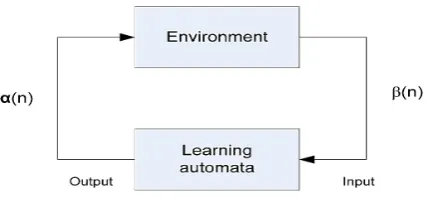
An adaptive decision-making unit, a learn-ing automaton through repeated interactions with a random environment learns how to choose the optimal action among a finite set of allowed actions to improve its performance. The action is chosen randomly on the basis of a probability distribution kept over the action-set, and the input to the random environment is the given action at each instant. The taken action is responded by the environment with a reinforce-ment signal. The action probability vector is up-dated based on the reinforcement feedback from the environment. A learning automaton tries to find the optimal action, from the action-set, with a minimized average penalty received from the environment.
The environment is defined by a triple E ≡ {α, β, c}, where α ≡ {α1, α2, . . . , αr } is the finite set of the inputs, β ≡ {β1, β2, . . . , βm} is the set of the values the reinforcement signal can take, and c ≡ {c1, c2, . . . , cr } denotes the set of the
penalty probabilities with element ci being asso-ciated with given action αi. If the penalty prob-abilities are constant, the random environment is considered a stationary environment; otherwise, it is called a non-stationary environment. On the basis of the nature of the reinforcement signal β, environments are also classified into: i) P-model, in which the reinforcement signal can only have two binary values 0 and 1, ii) Q-model with rein-forcement signals having a value in the interval [0, 1], and iii) S-model for which the reinforce-ment signal lies in the interval [a, b]. The two main types of learning automata are fixed- and variable-structure [6]. A variable-structure learn-ing automaton is represented by a triple < β, α, T >, where β, α and T are a set of inputs, actions, and the learning algorithm, respectively. The learning algorithm is a recurrence relation used to modify the action probability vector. Let α(k) and p(k) denote the action chosen at instant k and the action probability vector, respectively. The recur-rence equation shown by (1) and (2) is a linear learning algorithm by which the action probabil-ity vector p is updated. Let αi (k) be the action chosen by the automaton at instant k.
(1)
(2)
If the chosen action α_i (k) is rewarded by the random environment, Eq. (1), and if not, Eq. (2) is used. r is the number of actions chosen by the automaton; a(k) and b(k) are respectively the reward and penalty parameters, determining the amount of increases and decreases of the action probabilities. If a(k) = b(k), the recurrence equa-tions (Eqs.1-2) are called linear reward-penalty (L R−P) algorithm; if a(k) >> b(k), the equations are called linear reward-ε penalty (L R−εP), and
finally, if b(k) = 0, they are called linear reward-inaction (L R−I ). For the latter, the action prob-ability vectors remain unchanged when the taken action is penalized by the environment. In the unicast routing algorithm presented in this paper, each learning automaton uses a linear reward-inaction learning algorithm to update its action probability vector.
Learning automata have been found to be useful in systems operating in environments with incomplete information, and have also been proved to perform well in dynamic environments of wireless, ad-hoc and sensor networks. A group of learning automata can cooperate to cope with many hard-to-solve problems like combinatorial optimization problems in computer networks [16-19]. Here, we have used the learning automata be-cause of its simple structure and lack of informa-tion on the environment and sensor performance.
DISTRIBUTED LEARNING AUTOMATA
The full potential of learning automata will be realized when a cooperative effort is made by a set of interconnected learning automata to achieve a group synergy. A network of intercon-nected learning automata collectively cooperat-ing to solve a particular problem is called distrib-uted learning automata (DLA) [17]. Formally, a DLA can be defined by a quadruple < A, E, T, A0 >, where A = {A1, . . . , An} is the set of learning automata, E ⊂ A × A is the set of the edges with edge e(i, j ) corresponding to action αj of the au-tomaton Ai, T is the set of learning schemes with which the learning automata update their action probability vectors, and A0 is the root automaton of the DLA from which the automaton activation is started. The operation of a DLA can be de-scribed as follows. First, the root automaton ran-domly chooses one of its outgoing edges (actions) according to its action probabilities, and activates the learning automaton at the other end of the selected edge. The activated automaton also ran-domly selects an action leading to the activation of another automaton. The process of choosing the actions and activating the automata is contin-ued until a leaf automaton interacting with the en-vironment is reached. The chosen actions, along with the path induced by the activated automata between the root and leaf, are applied to the ran-dom environment. Evaluating the applied actions, the environment emits a reinforcement signal to
the DLA. With the use of the learning schemes, the activated learning automata along the chosen path updates their action probability vectors on the basis of the reinforcement signal. The paths from the unique root automaton to one of the leaf automata are selected until the probability of choosing one of the paths sufficiently approaches unity. Each DLA has just one root automaton al-ways activated, and at least one probabilistically activated leaf automaton.
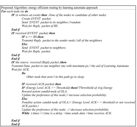
PROPOSED ALGORITHM
In this section, we propose an optimal rout-ing makrout-ing use of multi-path in wireless sensor networks, preventing energy depletion in nodes and direct data transmission to the destination node. Generally, the purpose is to decrease energy consumption in nodes, and prolong the network lifetime. There is a direct relation between energy consumption and the square of the distance; thus, one-hop connections with long distance consume more energy than multi-hop connections. There-fore, when learning automata is used to find mul-tipath to the sink, data transmission to the sink will only be done by the nodes of the selected path; consequently, direct data transmission will be pre-vented. Hence, we take advantage of learning au-tomata technique to choose the appropriate path.
Our proposed algorithm consists of the iden-tification, learning, and data sending phases, de-scribed in details as follows.
energy level to its own energy level. Other nodes add information of the reply packet to their own routing table, and forward the packet in all the networks.
Fig. 2. Structure of Reply packet
Generally, intermediate nodes after receiving the reply packet act as follows:
• The ID sender, hop count and energy level are entered in their routing table; that is, they enter their ID as sender node and set their energy level in the considered field.
• (Select Prob) Field shows the probability of the selection path based on the input informa-tion and Eq. 3.
• Each node receiving the information of the re-ply packet adds one hop to the number of hops and sends this packet to the next node.
• If a node receives only one reply packet, adds its information to the routing table, and con-siders its vector probability to be 1.
• If a node receives several packets, it adds their information to the routing table, and calculates the probability of selecting each path using Eq. 3.
(3)
Where Pi is the probability of selecting neigh-bor i; HOPcounti is the number of hops between neighbor i and the sink node; energy level i is the energy level of neighbor i; HOPcountj is the num-ber of hops between neighborj and the sink, and n is the size of the routing table.
• Routing tables include five fields: the next ID node, selection probability, energy level of the next node, hop count to the destination, and wake situation field which is important in the data sending phase(as shown in Figure 3).
Fig. 3. Structure of Routing table
Indeed, wake situation field in the rout-ing table expresses that the data is transferred from this path which is assigned first as false, and turns to true when the data passes from the path. Therefore, in the data sending phase, if
the nodes’ Wake situation field is False, they go to sleep.
Learning phase
In the learning phase, at the course of send-ing a data packet, a source node acts on the ba-sis of its obtained information from the previous phase; that is, each node has learning automata; the number of its actions is based on the number of node’s paths. The next node is selected based on the path selection, probability resulted from Eq. 3. Obviously, first, the shortest path has more chances because we initially consider the energy of all nodes the same, but after continues consuming of the shortest path, the nodes resid-ed on it waste their energy. This problem will be solved if we use learning automata and the multi-path idea. Hence, energy will be balanced in the network, too. Selecting each action will be equivalent to selecting its path. When each node is ready to send data, its learning autom-ata selects one of those paths. Then this node sends data to the sink node via this path. The data packet in addition to the considered data includes the id source, id destination, and send-ing source fields. The source node assigns the fields, and then sends the packet in on the path. N parameters are introduced for decreasing the number of the transmitted packets between the nodes, and for conserving energy. Each node se-lects a path through which sends n data packets. On the other hand, the destination node, receiv-ing n data packets, sends only one Ack packet to the source. As a result, the number of the control packets will be decreased, and energy consump-tion will be conserved, too. Receiving data, the sink node sends Ack packets through the same path to the source node. It is also defined for the source node whether the existing energy in each node related to the selected path is less than the threshold or not, and the source node consid-ers it as the response of the environment to the chosen action.
Therefore, the response of the environment to automata action is as follows. If the amount of the energy level in Ack packet is higher than the threshold, this action is rewarded and the vector probability of this path will increase; that is, the vector probability in the routing table is updated by the learning automation.
The threshold is the average energy calculat-ed in the first phase as the energy of the nodes in all paths up to the source node. If the energy of all the nodes resided on the path is less than the average energy of the other nodes on paths, this action is penalized by the learning automata, and also the vector probability is decreased. Accord-ing to these criteria, when the environment is P model, βi =0, the action is rewarded; otherwise, the action is penalized.
(5) Data sending phase (sleep or wake of nodes)
Normally, a sensor radio has four operating
modes including transmission, reception, idle lis-tening and sleep. It has been found that the high-est power consumption is due to transmission and, in most cases, the power consumption in the idle mode is approximately the same as the receiving mode [1]. On the contrary, the energy consumption in the sleep mode is much lower. The environment coverage phase is associated with inactive nodes leading to conserving energy. A path is selected if its vector probability is more than that of the others. In the learning phase, the optimal route is defined using the learning automata; thus, during the trans-mission phase, it is possible to decide about the time of deactivating nodes according to the wake situation field. The delay time is calculated as the time interval between sending the data and receiv-ing the confirmation of the returnreceiv-ing Ack packet. In this particular time, all other nodes not residing on this path go to sleep. This time depends on the
Fig. 5. Proposed algorithm
number of the hop counts. After finishing this time, sensors wake up and convert to idle state; it should be noted here that it is possible for the nodes to be in the idle state in this time; however, the idle state consumes more energy than the sleep mode. There-fore, in this algorithm, the nodes which are not on the data passing path go to the sleep state, and after the data is sent, they again convert to the idle state and wait for the next event. It is remarkable that those nodes sensing an event have almost the same data to be sent. Hence, it is possible to consider one node as a source node for sending data.
NETWORK MODEL
Wireless sensor network (WSN) includes a large number of sensor nodes dispersed in a sen-sor field. We consider N as the total number of sensor nodes. Additionally, no assumptions are made about the network diameter and density. We consider the following properties of the sen-sor network:
• The sensor nodes are static; in the majority of applications, sensor nodes have no mobility.
• Initially, all sensor nodes are charged with the same amount of energy.
• Links are bidirectional.
• The computation and communication capa-bilities are the same for all network nodes. Moreover, it is not feasible to recharge nodes’ batteries. For example, in a battlefield, sensor nodes are dispersed in a large target area where reaching and recharging them is extremely dif-ficult and dangerous. This motivates us to de-sign a protocol that is energy aware in order to prolong the lifetime of the network.
• Sensor nodes do not require GPS-like hard-ware; that is, they are not location-aware.
• Sensor nodes are not location-aware as re-gards to information sinks. Additionally, they have no knowledge about how many informa-tion sinks exist.
• The network “dies” when any of its sensors depletes its energy.
A GENERAL EXAMPLE
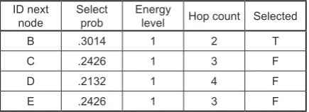
In Figure 6, assume node A observes an event in its environment (in its sensing range), and is selected as a source node among the others (since they have the same data). B, C, D and E nodes are neighbors of the source node. They are resided
in the transmission range of A. Node A sends an event pack to BS via one of its neighbors, and awaits for a reply packet. After receiving the reply packet of the sink, the other nodes justify their own routing (Table 1). Then, node A sends the data based on the selected probability field to the next node. As you can see in this example, the selection probability of node B is more than the other nodes, and the data is sent from this path. The selected field of B is set as true. The process of selecting nodes continues to the sink node by the learning automata. Then, the situation field of all the chosen paths having had higher prob-abilities than the other paths is set as True. These nodes having false field stay in the sleep mode (at the time period between sending the data and re-turning Ack packet); within this period, the nodes are in the sleep mode; hence, energy is conserved, and as compared to other similar methods [12– 15], the network life time is increased.
Table 1. Routing table example in 1 hop ID next
node Select prob Energy level Hop count Selected
B .3014 1 2 T
C .2426 1 3 F
D .2132 1 4 F
E .2426 1 3 F
SIMULATION PARAMETERS
The following metrics were considered for comparative evaluation of the above mentioned protocols.
The simulation experiments were carried out in NS-2 [20]. The simulation settings for the ex-periments were as follows.
a) Terrain dimensions: 200 × 200 m, b) Simulation time: 0-500 seconds, c) Number of nodes: 50-300, d) Speed of the mobile nodes: 0,
e) Underlying MAC protocol: IEEE 802.11, f) Channel: /Wireless,
g) Propagation: TwoRayGround, h) Network type: WirelessPhy, i) Queue: DropTail/PriQueue, j) Antenna: OmniAntenna,
k) Topography 700; # X dimension of the topog-raphy 700; # Y dimension of the topogtopog-raphy.
SIMULATION RESULTS
In our work, we assume a simple model where Eelec= 50 nj/bit to run the transmitter or receiver circuitry and for the transmit amplifier. We also assume an r2 energy
loss due to channel transmission. Thus, the ener-gy needed to transmit a k-bit message a distance d using our radio model [21], is:
ETx (k,d) = ETx-elec(k) +ETx-amp(k,d)
ETx (k,d) = Eelec* k + ϵamp* k *d2 (6)
And the energy needed to receive this mes-sage is :
ERx (k) = ERx-elec(k)
ERx (k) = Eelec*k (7)
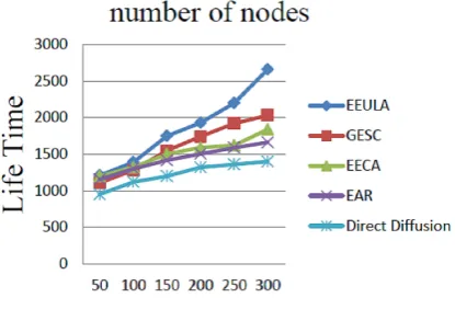
In this section, we compare our proposed routing protocol with the EAR, direct diffusion protocols [12-13], and with other algorithm such as the GESC and EECA [14-15]. The simulation experiments conducted in this section are con-cerned with investigating the efficiency of the distributed algorithms proposed for finding the best route of source to sink. In our experiments, the reinforcement scheme used for updating the action probability vectors is the LRP with reward and penalty parameters equal to 0.1. In order to generate the random graphs, a number of vertices were randomly distributed in a two-dimensional simulation area sized 200 m×200m. The reported results were averaged over 100 runs. The initial energy level of each node was 1 J; the radio trans-mit power was approximately two times the radio receive power. Our used performance measures were i) the impact of number of nodes to the life-time in Figure 7, ii) the impact of the sum of re-maining energy in nodes with time in Figure 8,
and iii) the impact of throughput with time in fig-ure9. Throughput is the average rate of successful packet delivery over a communication channel to sink. The EEULA and directed diffusion are dif-ferent from each other in the information transfer method. In directed diffusion, when the BS needs information, sends it as a request to the network, whereas in the EEULA, whenever sensor senses an event, sends it to BS. In both of them, all the communication is done with adjacent neighbors and there is no need to a special addressing mech-anism. Since in directed diffusion, the network starts its activity only at the time of BS’s request, and also there is no need to preserve the general topology of the network, this protocol is very ef-ficient in conserving energy; however, compared with our proposed algorithm, it suffers from a shorter lifetime and more energy consumption since it uses one path continuously.
When there is a need for sensors to periodi-cally send their information to the BS, these two protocols are useless. Therefore, they are not appropriate for applications such as controlling natural environment. Moreover, in directed dif-fusion, processing information to understand its conformity with the request results in energy consumption and delay in the network. Several
Fig. 7. Relationship between number of nodes and life time
of suboptimal paths are used in the EAR and EEULA to increase the network lifetime. In the EAR, these paths are chosen by a probability function related to energy consumption at the paths. The most important parameter taken into consideration in designing EAR was the network lifetime prolongation. A continuous use of a path leads to energy depletion of existing sensors on that path. Instead of one optimal path, we con-sider some suboptimal paths; however, just one of them is chosen in the EAR by a probability function and is used for a while. In both meth-ods, the routing phase and transferring data are the same, and the energy parameter is a function of sending and receiving the cost and amount of the remaining energy of sensors in the path; paths with high cost are not considered. In these two methods, the choice of sensors was based on their nearness to the destination. However, as compared with our proposed algorithm, in the EAR, whenever data is sent as local flooding to ensure the safety of the paths, it consumes more energy and decreases the network lifetime.
The EECA tries to discover the two short paths whose distances from each other are more than the interference range of the sensor node; it needs the nodes to be GPS-assisted and rely on the information provided by the underlying localization updating method. Thus, the network deployment cost and the communication over-head, specifically in large and dense wireless sensor networks, are increased. In addition, since signal variation in low-power wireless links is high, calculation of the interference range of the sensor nodes on the basis of distance may not result in accurate interference estimation [22]. Moreover, while transmitting data over minimum-hop paths can theoretically reduce the end-to-end delay and resource utilization, it in-creases the probability of packet loss and inten-sifies the overhead of packet retransmission over each hop in low-power wireless networks.
Clustering is suitable for large scale wireless sensor networks, and reduces the communica-tion overhead and exploits data aggregacommunica-tion in sensor networks using a topology management approach; however, in the GESC protocol, it creates many control packets during cluster cre-ation and maintenance, thus increasing energy consumption. The EEULA finds the best path through balancing energy consumption; there-fore, our algorithm with inactivating nodes con-serves energy, and consequently, increases the lifetime of the network. Moreover, the through-put had a considerable increase because there was no use of paths with low energy nodes. With the use of the learning automata, the best path is chosen for sending data, in which there is less energy consumption and also less distance to the sink node. It has been found that the learn-ing automata is very convenient to use in sen-sor networks since it has some features like low computational overhead, the ability to be used in distributed environments with inaccurate in-formation, and adaptation to changes in environ-ments [5]. Regarding energy limitation in sensor nodes and the need to reduce transmission of ex-cessive information to conserve energy, there is a tendency for sensor networks to use algorithms which are able to act distributed with local infor-mation. The present algorithm takes the advan-tage of automata to reduce energy.
CONCLUSION
In this paper, we presented a unicast ener-gy-aware routing protocol called EEULA. To balance energy consumption between nodes in the network, the present protocol makes use of learning automata to find suitable paths for send-ing data. The advantages of the presented proto-col include i) preventing continues consumption of the special path and waste of energy, ii) se-lecting the best path at different times by learn-ing automata, and iii) managlearn-ing energy with de-creasing control packet and inactivating nodes in the delay time.
Acknowlegements
This research was supported by the Shoush-tar Branch Islamic Azad University of the Islamic Republic of Iran through a grant to Ali Azimi So-tudeh Kashani. The author wants to express their gratitude for this support.
REFERENCES
1. Akyildiz F., W. Su, Y. Sankarasubramaniam and E. Cayircl, A survey on sensor networks, in: Proceed
-ings of the IEEE Communication Magazine, 40, August 2002, 102–114.
2. Anastasi G., M. Coti, M. Frrancesco, A. Passarella,
Energy conservation in wireless sensor networks: A
survey, Elsever, Ad Hoc Network, 2009, 537–568. 3. Pottie G. and W. Kaiser, Wireless integrated net
-work sensors, Communication of ACM, 43, 2000, 51–58.
4. Braginsky D., and D. Estrin, Rumor Routing
Algo-rithm for Sensor Networks, First ACM Workshop on Sensor Networks and Applications, October 2002, 22–31.
5. Narendra K.S., K. S. Thathachar, Learning autom -ata: An introduction, Printice- Hall, 1989.
6. Narendra K.S., M. A. L.Thathachar, Learning au
-tomata a survey, IEEE transactions on Systems, Man and Cybernetics, 4, July 1974.
7. Al-Karaki J.N. and A. E. Kamal, Routing tech -niques in wireless sensor networks: a survey, In
IEEE Wireless Communications, 11, 2004, 6–28.
8. Chang J.H. and L. Tassiulas, Energy conserving
routing in wireless ad-hoc networks, in Proc. of
IEEE INFOCOM, Israel, Mar 2000, 22–31.
9. Papadimitriou and L. Georgiadis, Energy-aware
Routing to Maximize Lifetime in Wireless Sen
-sor Networks with Mobile Sink, 13th International Conference on Software, Telecommunications and Computer Networks, SoftCOM, September 2005. 10. Niu Xiaoguang, Tao Zhihua, Wu Gongyi, H.
Changcheng, Li Cui, Hybrid Cluster Routing: An Efficient Routing Protocol for Mobile Ad Hoc Net
-works, Communications, IEEE International Con
-ference, 8, 2006, 3554–3559.
11. Ilyas M. and I. Mahgoub, Handbook of Sensor Networks: Compact Wireless and Wired Sensing Systems, in: Proceedings of the CRC Press, Lon
-don, Washington, D.C., 2005.
12. Shah R. and J. Rabaey, Energy Aware Routing for Low Energy Ad Hoc Sensor Networks, in Proceed
-ings of the IEEE Wireless Communications and
Networking Conference (WCNC), Orlando, FL, March 2002.
13. Intanagonwiwat Ch., R. Govindan, D. Estrin, Di
-rected Diffusion: A Scalable and Robust Commu
-nication Paradigm for Sensor Networks, IEEE/ ACM Transactions on Networking (TON), ISSN 1063-6692, 2 (1), 2003, 2–16.
14. Dimokasa N., D. Katsaros, Y. Manolopoulos. En
-ergy-efficient distributed clustering in wireless sen
-sor networks, J. Parallel Distrib. Comput, 2010. 15. Wang Z., Bulut E., Szymanski B.K. Energy Effi
-cient Collision Aware Multipath Routing for Wire
-less Sensor Networks. In Proceedings of the 2009 IEEE International Conference on Communications (ICC’09), Dresden, Germany, June 2009, 91–95. 16. Torkestani Akbari J., Meybodi M.R., Clustering
the wireless ad-hoc networks: A distributed learn-ing automata approach, Journal of Parallel and
Dis-tributed Computing, Elsevier Publishing Company (in press), 2010.
17. Torkestani Akbari J., Meybodi M.R. Learning
automata-based algorithms for finding minimum
weakly connected dominating set in stochastic
graphs, Int J Uncertain Fuzziness Knowl-Based Syst (to appear), 2010.
18. Torkestani Akbari J., Meybodi M.R. A new ver-tex coloring algorithm based on variable
action-set learning automata, J Comput Inf, 29 (3), 2010, 1001–1020.
19. Torkestani Akbari J., Meybodi M.R. Mobility-based multicast routing algorithm in wireless mobile ad hoc networks: a learning automata
ap-proach, J Comput Commun 33, 2010, 721–735. 20. The Network Simulator-ns2. http://www.isi.edu/
nsnam/ns/.
21. Heinzelman W., A.Chandrakasan, and H. Bal
-akrishnan, Energy-Efficient Communication Pro
-tocol for Wireless Microsensor Networks, Pro
-ceedings of the Hawaii International Conference on System Sciences, IEEE, 2000.
22. Baccour N., Aa A.K., Mottola L., Youssef H., Boa