126
Iranian (Iranica) Journal of Energy & Environment
Journal Homepage: www.ijee.net
IJEE an official peer review journal of Babol Noshirvani University of Technology, ISSN:2079-2115
Anomaly Detection in Smart Homes Using Deep Learning
M. Moallem*, H. Hassanpour, A. Pouyan
Faculty of Computer Engineering and Information Technology, Shahrood University of Technology, Shahrood, Iran
P A P E R I N F O
Paper history:
Received 04 Febraury 2019
Accepted in revised form 24 June 2019
Keywords:
Anomaly Detection Beam Search Deep Learning
Long Short Term Memory Smart Homes
A B S T R A C T
Smart homes enable many people, especially the elderly and patients, to live alone and maintain their independence and comfort. The realization of this goal depends on monitoring all activities in the house to report any observed anomaly immediately to their relatives or nurses. Anomaly detection in smart homes, just by existing data, is not an easy task. In this work, we train a recurrent network with raw outputs of binary sensors, including motion and door sensors, to predict which sensor will be switched on/off in the next event, and how long this on/off mode will last. Then, using Beam Search, we extend this event into k sequences of consecutive events to determine the possible range of upcoming activities. The error of this prediction i.e., the distance between these possible sequences and the real string of events is evaluated using several innovative methods for measuring the spatio-temporal similarity of the sequences. Modeling this error as a Gaussian distribution allows to assess the likelihood of anomaly scores. The input sequences that are ranked higher than a certain threshold will be considered as abnormal activities. The results of the experiments showed that this method enables the detection of abnormal activities with desirable accuracy.
doi: 10.5829/ijee.2019.10.02.10
INTRODUCTION1
The concept of smart homes as a subcategory of pervasive computing has long been the subject of interest in researchers and industrialists . Many researches and applications, such as home automation [1], optimal
energy consumption planning [2], provision of
telemedicine services [3], and home security and detection of break-ins by intruders [4] have been undertaken in the context of smart homes. However, most of these studies have focused on daily activity recognition and learning the routine of life in a smart home, failing to consider the challenging problem of anomaly detection and the detection of abnormal behaviors.
Anomaly detection and recognizing abnormal behaviors are of paramount importance, specifically in behavior monitoring systems (BMS) that surveil patients and elderly. In BMS any deviation in the daily routine of the subject can be considered as a new complication, an unhealthy habit or trend, and or a change and decrease of the person’s abilities [5].
In the literature on machine learning, anomalies are classified into three groups: point anomaly, collective anomaly, and contextual anomaly [6]. Point anomalies usually manifest in the form of the disparity between the value of one or more separate points and other values.
*Corresponding Author Email: [email protected] (Mahmoud Moallem)
These anomalies in the smart home affect numerica l static quantities such as the duration or frequency of doing a task. For example, a short night sleep or frequent visits to the bathroom can be considered as point anomaly. Cumulative anomaly refers to a set of values that are normative on their own but form anomaly when they are put together. The occurrence of this type of anomaly requires some kind of sequential (temporal -spatial) or semantic (graph) relationship among the relevant data. For example, leaving TV on, turning on the lights in the bedroom, and sleeping on the bed are not abnormal. However, the consecutive occurrence of these events may suggest that the residents have gone to bed without turning off the TV. Finally, in the contextual anomaly, a single instance of data is considered to be abnormal given its context. This type of anomaly includes several secondary and sometimes unrelated factors and is, therefore, more complex than other types. In smart homes, these factors often embrace spatial and temporal aspects [7, 8]. For example, sleeping in the bedroom is normal and sleeping in the kitchen is abnormal.
home anomaly detection. Section 4 describes the proposed method and outlines its major points. In section 5, we introduce a dataset from a real smart home and report the experimental results on this dataset. Finally , conclusions are drawn in section 6.
LITERATURE REVIEW
Research on anomaly detection has a long established history. Studies in this area, like many other branches of machine learning, originated from statistics. For example, Grubbs [9] and Enderlein et al. [10] in their seminal old books, have suggested powerful statistical methods for detecting anomalies. Among traditional methods of machine learning, many, including support vector machines [11], neural networks [12], and decision tree [13], have been used to anomaly detection. A crowd of these methods has been proposed by Chandola et al. [6] and Pimentel et al. [14].
In the field of smart homes anomaly detection, the concepts of routine actions and behavior modeling are the key concepts. Most researchers have tried to define and formulate normal behavior based on sensor data in an
unsupervised manner. An unsupervised learning
technique clusters the sensor data into different categories known as activities and identifys abnormalities as an observation which is deviated from the models of these pre-known activities. To do this, they use one or more of the following methods: logical methods, statistical methods, rule-based methods and machine learning methods.
The stochastic and non-deterministic nature of human activities complicates the modeling of these activities based on the common logic. Some researchers have attempted to take into account this uncertainty by using Bayesian logic and inference. For example, Ordonez et al. [15] defined three probabilistic features: sensor activation likelihood, sensor sequence likelihood, and sensor duration likelihood. Then they used these variables to model the behavior patterns of residents and to identify abnormalities in their behaviors. Using a Markov logic network, Hela et al. [16] have tried to integrate the power of first-order logic with the power of probability and using this probabilistic logic, search for abnormal activities and states in the uncertain space of the data in a smart home.
The hidden Markov model (HMM) is the most frequently used statistical method in processing smart home data. For example, Monekosso et al. [17] modeled sensors outputs sequences using HMM and considered rare observations as anomalies. This researchers did not use any contextual elements such as time or place, but divided a day into time intervals and, by creating a separate model for each interval, enhanced the accuracy of their method in recognizing abnormal activities.
Forkan et al. [18] also used the HMM to detect the anomalies. They used the high-level interpretation of sensor outputs, i.e., activities, as the model input. Also, they measured behavioral changes and health status of individuals respectively by analyzing their daily work and vital signs patterns. The outputs of these three models were given to a fuzzy system to make the final decision about the normality and abnormality of the situation. This complex approach suffers from two major drawbacks: 1) its precision largely depends on the method that is used to detect and extract activities from raw sensor outputs, 2) despite considering the contextual factor of time, it has failed to consider some important periodic variations such as holidays and weather conditions.
Another highly sophisticated method, which is a rule-based method was provided by Yuan et al. [19]. This model, in addition to binary sensors, employed several other sensors such as light, temperature, blood pressure, and sound sensor. The outputs of these sensors have been fused in various ways to form the sequence of activities. In the next step, the proposed system analyses these series using fuzzy logic and case-based reasoning. In this analysis, many contextual variables such as times, places, weekdays, as well as environmental and physiological factors of individuals were taken into account. Nevertheless, the reliance on this method on case-based reasoning means that it requires background knowledge and is not totally data-driven. In fact, Yuan et al. [19] have not provided any model for normal activities. For this reason, some of the cases should be classified into normal and abnormal by experts at the initial stage so that when the system starts to work, the history of activity flow is assessed through this classification, and the knowledge base of the system is updated.
The major weakness of the mentioned researches is that, they have relied on abstract concepts of activity and behavior. These concepts are very diverse for different people and at different times, so it is almost impossible to make a single definition of them. We tried directly use sensor data to detect anomalies, instead of using these high-level concepts. In this way, deep learning helps to extract the main features and frequent patterns automatically. It allows us to implicitly include these concepts in our model.
PRELIMINARIES
Recurrent neural networks, LSTM, and GRU
Recurrent Neural Networks are dynamic systems that maintain their internal state during process steps (for example, classification).
This feature is due to the circular communications that exist between adjacent layer neurons. In some models, these connections are seen in the same layer of neurons, or even in the context of a neuron with itself. These recurrent connections allow the network to retain the data of previous steps until the next steps. Thus, recurrent networks have a kind of memory, and therefore their computational model is more powerful than that of the feed forward neural networks [24].
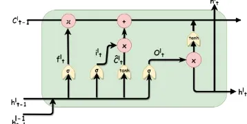
LSTM1 networks, instead of neurons use larger and more complex units called memory blocks. The main concept in each memory block is its state, which is a complex and nonlinear outcome of the input of block, output of adjacent blocks, state of the block in previous steps, and the state of the previous block. Each memory block is composed of a memory cell and some gates. The memory cell maintains the current state of the block and the gates handle the inward-outward flow of information . Figure 1 shows the structure of an LSTM memory block. As Figure 1 shows, each gate is a sigmoidal unit whose output ends up to a Hadamard or element-wise product. In LSTM architecture, gates receive input of the current block (xt) and output of the previous block (ht-1) as inputs, pass them through a sigmoid layer filter, and
Figure 1. The structure of an LSTM memory block
1 Long Short T erm Memory
2 Gated Recurrent Unit
produce a number between 0 and 1. This output defines the efficacy of the gate. The input gate determines which data should be stored in the memory cell, the forget gate decides how long these data should remain in the block, and the output gate specifies the data that should be mixed in the output of the block. Gers and Schmidhuber [26] added the current state of the block to the each gate`s input, named it as peephole connection, and created the most common type of LSTM blocks, known as peephole LSTM. The blocks used in this study are of original
type.
An LSTM block can be considered as an F function, which, by receiving the current input (xt), current state (c
t-1), and the output of the previous block (ht-1) generates the output of the current block (ht):
ℎ𝑡 = 𝐹 (𝑥𝑡 ,ℎ𝑡−1 , 𝑐𝑡−1) (1)
The F function follows the following steps since receives the input until the moment of the generation in the output:
𝑖𝑡= 𝜎 (𝑊𝑥𝑖 ∗ 𝑥𝑡 + 𝑊ℎ𝑖∗ ℎ𝑡−1 + 𝑏𝑖) (2)
𝐶̂ = tanh (𝑊𝑥𝑐∗ 𝑥𝑡 + 𝑊ℎ𝑐∗ ℎ𝑡−1 + 𝑏𝑐) (3)
𝑓𝑡 = 𝜎 (𝑊𝑥𝑓 ∗ 𝑥𝑡+ 𝑊ℎ𝑓∗ ℎ𝑡−1+ 𝑏𝑓) (4)
𝐶𝑡 = 𝑓𝑡 ⨀ 𝐶𝑡−1 + 𝑖𝑡 ⨀ 𝐶̂𝑡 (5)
𝑜𝑡 = 𝜎 (𝑊𝑥𝑜∗ 𝑥𝑡 + 𝑊ℎ𝑜∗ ℎ𝑡−1 + 𝑏𝑜) (6)
ℎ𝑡 = 𝑜𝑡 ⨀ tanh (𝐶𝑡) (7)
In the above relations, it, ft, and ot represent the input gate, the forget gate, and the output gate, respectively. W and
b are parameters of the model, i.e., weights of connections and biases. σ, Tanh, and ⨀ are also hyperbolic tangent functions, sigmoid, and the element -wise product operator, respectively.
The GRU2 structure proposed in 2014 by Cho et al. [27]
Multi-task learning
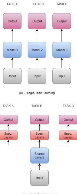
There are two methods for simultaneous prediction of two dependent and associated variables. In the first method, we consider them as two independent variables and develop separate models to predict each of them. But, in the second method, the variables simultaneously pass through shared layers, and then each variable is delivered to its specific layers. Each variable has its cost function and the training is done for minimizing an overall cost function that derived from the weighted sum of these functions. This method, called Multitask Learning [29], takes into account the dependence of the relevant variables. Multi-task learning has long been used in machine learning applications, including Natural Language Processing, Speech Recognition and Machine Vision [30]. Application of this method, especially for dependent variables, increases the accuracy of prediction and reduces the risk of overfitting. Figure 2 shows the difference between the usual single-task learning (or single learning) and multi-task learning (or simultaneous learning).
Since we intend to perform a simultaneous prediction of two variables: the next event label and the duration of the event, multi-task learning better suits our purpose and achieves higher performance and accuracy.
Figure 2. Single-task learning versus multi-tas k learning.
Anomalies in Smart Homes
Most of the smart home datasets, record sensor events in the following format:
ei = <T, S, A> (8)
In this triple, T is timestamp and stands for "sensor activation time", which is often expressed in seconds and includes date too; S stands for "Sensor Identifier" and can contain other information, such as the location or the object where the sensor is attached, and finally, A
represents "SensorValue". Since all of our sensors are binary, this value can be considered as ON or OFF. The index i in the definition of ei denotes that the order of
events is important.
However, we convert the sensor event ei into the
following triple:
ei = <T, SA, D> (9)
In this triple, T still stands for timestamp and SA is a string obtained by concatenating S and A values from the previous triple, which is called Event Label. The third element, D or duration, shows the time between the present and previous event. In other words:
Di= Ti - Ti-1 (10)
Naturally, this value is zero at the first event. For example, in our method, the triple <T5, M1, ON> will be converted into triple <T5, M1ON, T5-T4>.
A series of successive events such as E is called Episode: E = <e1, e2, e3, …., en> (11)
The order of an episode is determined by the activation time of its events (T). An episode can often be interpreted as an activity. For instance, if a person leaves the bedroom and go to the kitchen through a hallway and each of these locations has its motion sensor called e1, e2 and e3, then episode <e1, e2, e3> will be observed.
We define abnormal behavior as an episode in which:
has never been observed yet;
is rarely observed in the past;
is significantly away from the recent episodes. The above definitions of anomaly are only related to the events and the order of their occurrence, without considering temporal anomalies. There is another kind of anomaly in which:
an abnormal episode has already been seen, but its temporal coordinates are far different from the previous observations.
For example, several-hours interval between episodes e2 and e3 in the above example should be considered abnormal, as it may suggest that someone has suffered an accident before reaching to the kitchen.
THE PROPOSED METHOD
Figure 3. The overall scheme of the proposed method
which includes the following steps:
By concatenating S and A values, SA value is obtained.
The character string of SA is encoded. This encoding can be carried out by One Hot encoding or Word Embedding method.
By subtracting the current and the previous event timestamps, D is calculated.
Timestamp conversion is carried out in a way that periodicity, cycle, and the return of time are considered.
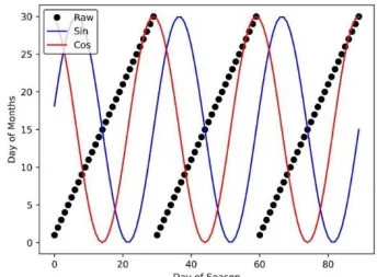
In explaining the last preprocess, it should be noted that applying common ways to express features like weekdays or months could lead to the confu sion of classifiers. As an example, using numbers 1 to 7 for weekdays may give the classifier the misperception that 4th and 5th days are more similar than the 1st and 5th days! The same holds true for days of month, even with more complication, as months lengths are different. So, it is generally preferable to use the Fourier transform for expressing the cycling and periodic variables. The above transformation formula, for example for a day's hours, is as follows:
a = h × (2π / 24) (12) This transformation maps hours into the surface of a circle. Thus, the difference between two hours is expressed as the angle between the two vectors created by this mapping, i.e. (cos (a), sin (a)). Figure 4 shows how the days of 3-months, in each of the above methods, is displayed.
In the next step, the input data is segmented into windows of length n and overlapping m, to convert the problem into a type of supervised classification. Each window is considered as X and the next event, i.e., en + 1, is considered as Y. Now, we must find a mapping that can guess the next event with high precision by receiving an n-events window.
F(<ei, ei+1, ei+2, …., ei+n>) = ei+n+1 (13)
We used LSTM and GRU networks with different structures to find the above mapping. Details of these structures are presented in s ection 5-2. It should be noted that all utilized networks predict the SAi + n + 1 and Di + n +
1 components of the next event, and the timestamp of this event, i.e., Ti+n+1, can be calculated by summing the temporal elements of the previous event, i.e., Ti+n + Di+n. After training the model by training data, we will have a predictive model that can predict the next event, i.e, et + 1, by receiving the input string <e1, e2, ..., et>. In time the detection of point anomalies; but, because we want to find collective and contextual anomalies, this criterion is not applicable to our issue. In other words, we are looking series applications, the distance between the predicted values and the real values is usually used as a measure for for a sequence of events that their occurrence at a specified time is considered as an anomaly. For this reason, after making the prediction, we add et + 1 to the beginning of the input string and remove the its first event (i.e. e1). Now we have a new t-fold episode, like <e2, e3,...,
et + 1> that can be used to predict the event in the next two steps, et + 2. By repeating this process, we bring a sequence of the subsequent probable events. This method, known as the recursive or iterative prediction, is a common practice in the literature on the sequences and time series [31]. The disadvantage of this method is that, despite its high precision in the first steps, its accuracy drops dramatically when the number of steps is increased, due to the accumulation of errors. For this reason, this approach is only suitable for predicting a limited horizon of upcoming events [31].
The distinctive feature of our work is that we use the Beam Search instead of using the usual greedy method to find the next step. Note that the proposed model at each step predicts a single number as duration or D, but the prediction of event label or SA is different. We use a Softmax function to predict this element in the last layer of our networks. The output of this layer is a vector whose length is equal to the number of existing labels and the value assigned to each item is equal to the probability of its occurrence.
At each step, we select the m labels that have the highest probability, and by adding D to them, and computing the associated T, we offer m suggestion for the following event. Then, we make iterative predictions with these m suggestions and create m*m proposals for the next two steps. By continuing this process in l iterations, we will end up having a full and balanced tree, with the depth l and m offspring per node. A complete traversing of all paths of this tree, from root to leaves, provides us with ml probable episodes along with the probability of each node. Now, using the Beam Search method, we can extract some possible sequences of events from these paths. The number of these sequences represents the desired value of k, which is called “beam size.”
Beam Search is a heuristic method that explores the tree of the upcoming states and expands only the nodes that are more likely to occur than others [32]. This method is based on Breath-First Search, meaning that it first generates all successors of the states at the current level. The difference here is that the beam search, arranges these nodes based on a target function f, and only stores a predetermined number of best states at each level. This number, known as beam size, is usually determined by temporal and computational - especially memory- limitations. Naturally, larger values will increase the required time and memory for running the program. As the beam-size approaches to infinity, the method gets closer to the Breath-First Algorithm. Bea m search is widely used in Text Mining and Natural Language Processing [33].
Now we have k event sequences of length l, which are likely to occur based on the available data. The distance between the real episode and this set can be considered as a prediction error and used to compute the Anomaly
Score. These strings contain a set of ordered tuples, in which an element - the event label - is discrete, and the other element -the duration - is continuous. For this reason, none of the methods used to calculate the distance between discrete sequences or time series are applicable to this case.
To calculate this distance, we use the method proposed by Park et al. [34]. In this study, four different similarity functions have been defined. These functions take into account all possible features concerning the differences and similarities of the above tuples. Then the weighted sum of them are used as the final s imilarit y criterion. These functions are expressed in Equations (14) to (18). In these equations, A and B refer to the two compared episodes and n denotes their lengths. Also, LCS is the Longest Common Substring of these two episodes, with the length k. Symbols | | and {{}} are also used to represent the length of a structure (e.g., a sequence) and the length of a MultiSet, respectively. A multiset is a set in which the elements may occur more than once and where several identical members do not reduce to one single member. Finally, S refers to the final similarity criterion:
𝑆(𝐴, 𝐵) = ∑4𝑖=1𝑤𝑖 𝑆𝑖 (14)
𝑆1= |𝐿𝐶𝑆𝐴,𝐵|
𝑘 (15)
𝑆2= | {{ 𝑥 | 𝑥 ∉𝐿𝐶𝑆 ,𝑥∈𝐴 𝑜𝑟 𝑥∈𝐵 }} |
𝑛 (16)
𝑆3= 1 − 𝑆𝑡
𝑡𝐶 (17)
𝑆4=
∑ 𝑀𝑖𝑛(𝑑𝑗,𝑑′𝑗)
𝑀𝑎𝑥(𝑑𝑗,𝑑′𝑗) |𝐿𝐶𝑆|
𝑗=1
𝑘
(18)
In Equation (17), the function St is defined as:
𝑆𝑡= ∑ |𝑡𝑗− 𝑡
′
𝑗|
|𝐿𝐶𝑆| 𝑗=1
𝑘 (19)
It should be noted that among the above criteria, S3 (Equation (17)) and S4 (Equation (18)) contains the concept of time. In these relations, tj, t'j, dj and d'j represents the timestamp and duration of two events of episodes A and B, which have the same position in the LCS. Finally, tC is the time constant in seconds, which depends on the period under study. For example, to study a 24-h interval, this constant is equal to 86,400. The value of each sub-function of Si is normalized to a number within 0 and 1. Then, the weighted sum of these values is used as the final criterion. By naming this function like F, the difference between the k-member set of the predicted sequences and the real episode will be as follows:
𝑑 = 1
𝑘 ∑ 𝑓(𝐸, 𝑆𝑖) 𝑘
𝑖=1 (20)
window. This vector is modeled as a Gaussian distribution of N(μ, Σ) [35]. Thus, the probability of observing pt error at point et is obtained by calculating the value of N at the point et. We use the Maximu m Likelihood Estimation method to calculate μ and Σ values. Now any input window whose pt value is greater than the threshold t is considered as an anomaly. The value of this threshold can be determined either statically based on the existing observations or dynamically by maximizing the Fβ criterion.
EXPERIMENTS
Dataset
The dataset used in this study was taken from the Center for Advanced Study of Adaptive Systems (CASAS) located at Washington State University. This center is one of the most prestigious smart home study centers. The contents of the dataset were collected in the course of 220-days- since November 4, 2010, to June 11, 2011 - from round-the-clock monitoring of an old woman. To construct this dataset, called Aruba [36], 40 sensors including motion sensors, door closure sensors, and temperature sensors were used. The Aruba dataset contains 11 types of daily activities and 1,719,553 sensor events. Since our study only deals with binary sensors, we eliminated the set of temperature events, reducing the number of these rows to 1,602,818. An example of the contents of Aruba is shown in Figure 5. This dataset has been primarily designed to recognize and classify daily activities, so there are no distinct and labeled anomalies in it. For this reason, we considered its data as normal, and accordingly, generated 100 sample anomalies manually. These records are in shape of episode form and contain one types of anomalies mentioned in section 3-3. Regretfully, there is currently no public and standard dataset for detecting anomalies in smart homes. For this reason, manual adding of anomalies to public ADL datasets, which were basically designed for activity recognition, is a conventional method utilized by many researchers, including Ye et al. [37], Ordonez et al. [15], and Shin et al. [38].
Implementati on
We conducted a series of experiments to evaluate the proposed method. These experiments differ in criteria such as the length of the input window, the overlapping
Figure 5. A part of Aruba dataset
of these windows, the number of output vectors, and the beam size (the number of output strings of the beam search). Table 1 summarizes the characteristics of these experiments.
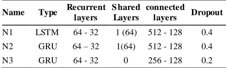
We also created various networks as the prediction and anomaly detection model that vary in the type of elements (LSTM or GRU), the number of blocks, the number of layers, the specifications of the fully connected (Dense) layers and Dropout. Table 2 summarizes the characteristics of these networks.
Irrespective of these differences, other learning, and experimental parameters are identical in the experiences. Input data are divided into two sections of 70 and 30%. The first part constitutes the training set and the second part, after the injection of manually generated anomalies, has been used as the test set. The data were delivered to the models in 100-fold batches (batch size = 100), and each network was trained 50 times (epochs = 50). Finally , in all cases, the learning rate was 0. 0025, and the cross-entropy function was used as the network loss function. In addition to the above structures, we also used the One-Class Support Vector Machine (OC-SVM). This method has been used in several studies for detecting anomalies in smart homes.
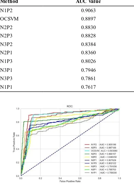
For the comparison of these methods, we used the Receiver Operating Characteristic (ROC) curve and Area Under the Curve (AUC) [39]. Common measurement criteria, such as precision, accuracy, recall and even the F1 measure, which are frequently used to analyze classification methods, lack the required efficacy and flexibility in detecting anomalies. For this reason, in most of the researches undertaken in this area, ROC and AUC criteria have been adopted [40, 41]. Table 3 shows the AUC values for different experiences. Figure 6 also shows the ROC graph for the same experiences.
These experiments showed that LSTM networks work better. Of course, the training time of LSTM networks is much longer. The superiority of the P2
TABLE 1. Features of experiments
Name Length of the input window
Overlapping
% output vectors Number of Beam
size
P1 4 0 5 6
P2 8 25 8 6
P3 12 50 10 8
TABLE 2. Features of the applied networks
Name Type Recurrent layers
S hared Layers
connected
layers Dropout
N1 LSTM 64 - 32 1 (64) 512 - 128 0.4
N2 GRU 64 – 32 1(64) 512 - 128 0.4
experiment shows that the length of the input window has a significant effect on the improvement of the prediction and the ability to detect abnormalities. In fact, when splitting the input entries into sliding windows, the length of each window should be close to the average length of the user's activity. Also, the overlapping of these windows should be selected so that abnormalities are not considered as normal strings by replication and distribution among adjacent windows. To adjust these parameters, we need to consider the statistics of the data used.
These experiments showed that LSTM networks work better. Of course, the training time of LSTM networks is much longer. The superiority of the P2 experiment shows that the length of the input window has a significant effect on the improvement of the prediction and the ability to detect abnormalities. In fact, when splitting the input entries into sliding windows, the length of each window should be close to the average length of the user's activity. Also, the overlapping of these windows should be selected so that abnormalities are not considered as normal strings by replication and distribution among adjacent windows. To adjust these parameters, we need to consider the statistics of the data used. Increasing the number of output vectors and the
TABLE 3. Features of the applied networks
Method AUC value
N1P2 0.9063
OCSVM 0.8897
N2P2 0.8830
N2P3 0.8828
N3P2 0.8384
N2P1 0.8360
N1P3 0.8026
N3P1 0.7946
N3P3 0.7861
N1P1 0.7617
Figure 6. ROC graph for different experiences
beam size raise the runtime, but in contrast, it improves the variety and quantity of guesses. As a result, the distance of the proposed set will be reduced to the actual episode. This is probably why the P3 experience has produced good results. We also found that the use of multi-task learning and using shared layers to jointly predicting the next event label and its timestamp increases the accuracy of prediction and the likelihood of anomaly detection. The weakness of the N3 model results is due to the lack of these layers.
All the required programs are written in Python, using Tensorflow and Keras libraries. These programs were run on Linux Mint, relying on the features of the CUDA 8 library to utilize the graphics card capability. The computer was also equipped with an NVidia GeForce 920 MX graphics card with 256 CUDA cores, a quad -core Intel Core i7 7500U 2.7 GHz processor and an 8GB physical memory.
CONCLUSIONS
In this article, we proposed the use of recurrent networks for anomaly detection in smart homes. Our proposed method does not require any activity recognition mechanism, and the raw output of sensors is received as the inputs. Since the common anomalies in smart homes are of contextual and collective types, we selected some of the most probable upcoming sequences of events using beam search so that their comparison with real episode alerted us about the possible occurrence of the anomalies.
The results of our experiments showed that this method was successful in detecting various anomalies and identifying the range of them with desirable precision. Based on our experience, LSTM networks outperform GRU networks. The truth of the last proposition, and the values of other parameters, such as the size of the input window, their overlapping percentage, the beam size of beam search, among other things, should be examined separately for each dataset.
REFERENCES
1. Withanage, C., R. Ashok, C. Yuen, and K. Otto, 2014. A comparison of the popular home automation technologies, In 2014 IEEE Innov. Smart Grid Technol. - Asia (ISGT ASIA), pp: 600–605.
2. Zhou, B., W. Li, K.W. Chan, Y. Cao, Y. Kuang, X. Liu and X. Wang, 2016. Smart home energy management systems: Concept, configurations, and scheduling strategies. Renewable and Sustainable Energy Reviews, 61: 30–40.
3. Majumder, S., E. Aghayi, M. Noferesti, H.
Memarzadeh-Tehran, T. Mondal, Z. Pang and M.J. Deen, 2017. Smart Homes for Elderly
Healthcare-Recent Advances and Research
Challenges.Sensors Vol. 17, no. 11 (2017): 2496.
4. Dahmen, J., B.L. Thomas, D.J. Cook and X. Wang, 2017. Activity learning as a foundation for security monitoring in smart homes. Sensors (Switzerlan d ), 17(4): 1–17.
5. Eisa, S. and A. Moreira, 2017. A behaviour monitoring system (BMS) for ambient assisted living. Sensors (Switzerland), Vol. 17(9): (2017): 1946.
6. Chandola, V., A. Banerjee, and V. Kumar, 2009. Anomaly detection. ACM Computing Surveys, 41(3): 1–58.
7. Hayes, M.A. and M.A.M. Capretz, 2014. Contextual anomaly detection in big sensor data. Proceedings - 2014 IEEE International Congress on Big Data, BigData Congress 2014, 64–71.
8. Han, J., M. Kamber, and J. Pei, 2011. Data Mining: Concepts and Techniques. 3rd ed. Morgan Kaufmann Publishers Inc.
9. Grubbs, F.E., 1969. Procedures for Detecting Outlying Observations in Samples. Technometrics, 11(1): 1–21.
10. Enderlein, G., 1987. Hawkins, D. M.: Identification of Outliers. Chapman and Hall, London – New York 1980, 188 S., £ 14, 50. Biometrical Journal, 29(2): 198.
11. Ma, J. and S. Perkins, 2003. Time-series novelty detection using one-class support vector machines, In Proc. Int. Jt. Conf. Neural Networks, 2003., IEEE, pp: 1741–1745.
12. Tavares Ferreira, E.W., G. Arantes Carrijo, R. de Oliveira and N. Virgilio de Souza Araujo, 2011. Intrusion Detection System with Wavelet and Neural
Artifical Network Approach for Networks
Computers. IEEE Latin America Transactions, 9(5): 832–837.
13. Depren, O., M. Topallar, E. Anarim, and M.K. Ciliz, 2005. An intelligent intrusion detection system (IDS) for anomaly and misuse detection in computer
networks.Expert systems with Applications Vol. 29, no. 4 (2005): 713-722.
14. Pimentel, M.A.F., D.A. Clifton, L. Clifton, and L. Tarassenko, 2014. A review of novelty detection. Signal Processing, 99: 215–249.
15. Ordonez, F.J., P. de Toledo and A. Sanchis, 2015. Sensor-based Bayesian detection of anomalous living patterns in a home setting. Personal and Ubiquitous Computing, 19(2): 259–270.
16. Hela, S., B. Amel, and R. Badran, 2018. Early anomaly detection in smart home: A causal
association rule-based approach. Artificia l
Intelligence in Medicine, Vol. 91 (2018) 57-71.
17. Monekosso, D.N. and P. Remagnino, 2010.
Behavior analysis for assisted living. IEEE
Transactions on Automation Science and
Engineering, 7(4): 879–886.
18. Forkan, A.R.M., I. Khalil, Z. Tari, S. Foufou and A. Bouras, 2015. A context-aware approach for long-term behavioural change detection and abnormality prediction in ambient assisted living. Pattern Recognition, 48(3): 628–641.
19. Yuan, B. and J. Herbert, 2014. Context-aware
Hybrid Reasoning Framework for Pervasive
Healthcare. Personal Ubiquitous Comput., 18(4): 865–881.
20. Novak, M., M. Binas and F. Jakab, 2012.
Unobtrusive anomaly detection in presence of elderly in a smart-home environment. Proceedings of 9th International Conference, ELEKTRO 2012, (June 2016): 341–344.
21. Moshtaghi, M., I. Zukerman, and R. Andrew Russell, 2015. Statistical models for unobtrusively detecting abnormal periods of inactivity in older
adults. User Modeling and User-Adapted
Interaction Vol. 25, no. 3 (2015): 231-265.
22. Paudel, R., W. Eberle, and L.B. Holder, 2018. Anomaly Detection of Elderly Patient Activities in Smart Homes using a Graph-Based Anomaly Detection of Elderly Patient Activities in Smart Homes using a Graph-Based Approach. (July): https://scholar.google.com/citations?user=v_Lx8lY AAAAJ&hl=en&oi=sra
23. Jakkula, V. and D.J. Cook, 2011. Detecting Anomalous Sensor Events in Smart Home Data for Enhancing the Living Experience. AAAI Workshop on Artificial Intelligence and Smarter Living The Conquest of Complexity, (June 2015): 33–37.
24. Lipton, Z.C., J. Berkowitz and C. Elkan, 2015. A Critical Review of Recurrent Neural Networks for Sequence Learning. 1–38. arXiv:1506.00019v4
26. Gers, F.A. and J. Schmidhuber, 2000. Recurrent nets that time and count, In Proc. IEEE-INNS-ENNS Int. Jt. Conf. Neural Networks. IJCNN 2000. Neural Comput. New Challenges Perspect. New Millenn., IEEE, pp: 189–194 vol.3.
27. Cho, K., B. van Merriënboer, C. Gulcehre, F. Bougares, H. Schwenk and Y. Bengio, 2014. Learning Phrase Representations using RNN
Encoder-Decoder for Statistical Machine
Translation. arXiv preprint
arXiv:1406.1078 (2014).
28. Chung, J., C. Gulcehre, K. Cho and Y. Bengio, 2014. Empirical evaluation of gated recurrent neural networks on sequence modeling, In NIPS 2014 Work. Deep Learn. December 2014,
29. Caruana, R., 1997. Multitask Learning. Machine Learning, 28(1): 41–75.
30. Collobert, R., R. Collobert and J. Weston, 2008. A unified architecture for natural language processing: Deep neural networks with multitask learning. 160-167.
31. Kline, D., 2004. Methods for Multi-Step Time Series Forecasting with Neural Networks. In Neural
network s in business forecasting, pp. 226-250. IGI
Global, 2004.
32. Reddy, D.R.( D. of C.S., 1977. Speech
Understanding Systems: A Summary of Results of the Five-Year Research Effort at carnegie-mello n university." Internal Document. August (1977).
33. Freitag, M., and Y. Al-Onaizan, 2017. Beam Search Strategies for Neural Machine Translation. arXiv
preprint arXiv:1702.01806 (2017).
34. Park, K., Y. Lin, V. Metsis, Z. Le and F. Makedon,
2010. Abnormal human behavioral pattern
detection in assisted living environments.
Proceedings of the 3rd International Conference on PErvasive Technologies Related to Assistive Environments - PETRA ’10.
35. Malhotra, P., L. Vig, G. Shroff, and P. Agarwal, Long Short Term Memory Networks for Anomaly Detection in Time Series. In Proceedings, p. 89. Presses universitaires de Louvain, 2015
36. Cook, D., 2010. Learning Setting-Generalize d Activity Models for Smart Spaces. IEEE intelligent
systems no. 99 (2010): 1.
37. Ye, J., G. Stevenson and S. Dobson, 2016. Detecting abnormal events on binary sensors in smart home environments. Pervasive and Mobile Computing, 33: 32–49.
38. Shin, J.H., B. Lee and K.S. Park, 2011. Detection of abnormal living patterns for elderly living alone using support vector data description. IEEE
Transactions on Information Technology in
Biomedicine : A Publication of the IEEE
Engineering in Medicine and Biology Society, 15(3): 438–448.
39. Fawcett, T., 2006. An introduction to ROC analysis. Pattern Recognition Letters, 27(8): 861–874.
40. Goldstein, M., M. Goldstein, and S. Uchida, 2016. A Comparative Evaluation of Unsupervised Anomaly Detection Algorithms for Multivariate Data. PLoS ONE, (April): 1–31.
41. Emmott, A., S. Das, T. Dietterich, A. Fern and W.-K. Wong, 2015. A Meta-Analysis of the Anomaly
Detection Problem. arXiv preprint
arXiv:1503.01158 (2015).