ISSN 1392–124X INFORMATION TECHNOLOGY AND CONTROL, 2007 Vol. 36, No. 1A, 1
A SysML requirements model for the 1992 ACC robust control benchmark
Fernando Valles-Barajas
Department of Information Technology, Faculty of Engineering, Universidad Regiomontana 15 de Mayo 567 Pte., C.P. 64000 Colonia Centro,
Monterrey, Nuevo Le´on, M´exico phone: +52 81 8220-4733
E-mail: [email protected], [email protected]
Abstract. In this paper a conceptual design for the software of control systems is presented. The design was made using requirements tables and requirements diagrams of SysML, which is a modeling language for modeling systems. The resulting design can be used to estimate the required effort to build software for control systems as well as to document and complement the textual requirements of control systems. The usefulness of this proposal is shown by making a conceptual design for the 1992 ACC robust control benchmark.
Key words:PSP, Software Design, Control Systems, SysML, Requirements Diagrams.
1. Introduction
The Personal Software Process1 (PSP) is a process that helps software engineers in produc-ing high quality software [4]. In this software pro-cess a software engineer needs to estimate the necessary effort to make a software product based on a requirements document. For this estimation, PSP recommends making a model which captures the essential characteristics of the system to be developed; this model is called in PSP concep-tual design. Once the estimation of the necessary effort is made, the conceptual design is detailed later using the four PSP templates (operational, functional, sate and logic templates) which model four different views of a system.
SysML is a modeling language that has several diagrams and is used to model systems [6]. One of the SysML diagrams is the requirements dia-gram, which is used to model, document, specify, and analyze the requirements of a system. Control systems are composed of hardware (sen-sors, computers, actuators) and software [5]. The latter is where control laws (for example PID, RST or GPC) are specified.
Motivation of the paper: the author of this paper proposes to make a conceptual design for the soft-ware of control systems based on a requirements document using requirements tables and SysML
requirements diagrams. The benefits of the pro-posal are:
• This design can be used to estimate the necessary effort to build software for control systems.
• This design will later serve to build a detailed design for the software of control systems using the four PSP templates. • A graphical model where requirements are
specified is added to the textual documentation of control systems. • A bridge between typical requirements
tools and tools that model the system elements is established. Using this bridge, when a requirement changes the model elements that suffer a change will easily be detected.
Related works: In [10] a requirements process for the software of control system is presented. This process is based mainly in the Rational Unified Process (RUP).
In [2] the specification and analysis of the require-ments for an avionic control system are given. This specification is based on formal methods. In particular the PVS language is used in the spec-ification and analysis phase.
The importance of the specification of control sys-tems requirements is shown by taking a look at the special issue on the modeling and analysis of the requirements for a light control system [8].
Structure of the paper: In Section 2 SysML re-ISSN 1392 – 124X INFORMATION TECHNOLOGY AND CONTROL, 2009, Vol. 38, No. 3
A SYSML REQUIREMENTS MODEL FOR THE 1992 ACC ROBUST
CONTROL BENCHMARK
Fernando Valles-Barajas
Department of Information Technology, Faculty of Engineering, Universidad Regiomontana 15 de Mayo 567 Pte., C.P. 64000 Colonia Centro, Monterrey, Nuevo León, México
e-mail: [email protected], [email protected] t
Abstract. In this paper a conceptual design for the software of control systems is presented. The design was made using requirements tables and requirements diagrams of SysML, which is a modeling language for modeling systems. The resulting design can be used to estimate the required effort to build software for control systems as well as to document and complement the textual requirements of control systems. The usefulness of this proposal is shown by making a conceptual design for the 1992 ACC robust control benchmark.
2 Fernando Valles-Barajas
contains the requirements in textual form for the 1992 ACC robust control benchmark. In section 4 a conceptual design of the control system ex-plained in sec. 3 is given using the SysML nota-tion. The last section presents some concluding remarks.
2. SysML
SysML is a modeling language that is based on UML and serves to model systems. It takes some of the UML diagrams (sequence, state ma-chine, use case and package diagrams), modifies some of them (activity, block definition and inter-nal block diagrams) and introduces new diagrams (requirements and parametric diagrams).
2.1. The requirements diagram
A requirement is a capability or condition that a system must satisfy. In SysML the require-ments are represented as model elerequire-ments; being more specific, the requirements in a requirements diagram are represented as abstract classes with-out operations. A requirement has properties to specify its unique id and its description; the lat-ter property is called “text”.
A requirement is represented as a stereotyped class using the stereotype requirement with a
unique id and a textual description.
The relationships between requirements in a re-quirements diagram are: containment, which is represented using a cross hair, and the stereo-typed dependencies deriveReq, copy and refine. There are other relations between
re-quirements and model elements. For example, the
satisfyrelationship is used to specify a model
element that satisfies some particular require-ment. The verifyrelationship is used to assign
a test case to a model element.
The containment relationship is used to decom-pose a requirement into sub requirements; so a complex requirementreq1 can be decomposed in, for instance, requirements req2 and req3. The containment relationship is useful to deal bet-ter with the implementation of complex require-ments. Requirements related to the containment relationship form a hierarchy. This relationship is represented by a small circle with a cross collo-cated near the complex requirement.
Thecopyrelationship is used to reuse
require-ments in different models. It is important to men-tion that the copy relationship is necessary,
because in SysML a model element can not be drawn in two different diagrams.
The deriveReq relationship can be used to
specify when one requirement is a derivation from another requirement. This relationship expresses the relation between a particular requirement and the requirements that support this requirement. The refinerelationship can be used to specify
an element that refines a requirement; for exam-ple a use case or a sequence diagram can be used to refine a requirement.
It is possible to define the design or implemen-tation model which satisfies one or more require-ments by using thesatisfy relationship.
Test cases can be associated with a requirement by using the verifyrelationship. The notation
for a test case is similar to the notation of a re-quirement; a stereotyped class with the stereo-typetestCaseis used to represent a test case.
The rationale construct can be attached to a
requirement or to a relation to support, for ex-ample, the decision that was taken to satisfy a requirement using a component.
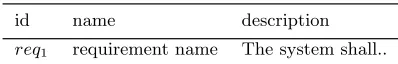
A requirements diagram is a graphical form to represent the requirements of a system. The re-quirements of a system, the relationships between them and other elements can also be represented in tabular form. Table 1 shows an example of a table that specifies the requirements of a system. This table contains anid, aname and a descrip-tion of the requirements, but this table may also contain the relationships between them.
Table 1. Tabular form for the requirements
id name description
req1 requirement name The system shall..
3. A study case
Fig. 1 presents a typical configuration for a control system. In this figure y(k) is the output
Gc(z−
1
) Gp(z−
1
) j
Σ
-j Σ
? 6
-d2(k)
n(k)
e(k)
yref(k)
Σ -Σj? y-(k)
u(k)
-? -d1(k)
h
Fig. 1. Typical configuration for a control system
variable, u(k) is the input variable, e(k) is the
F. Valles-Barajas
A SysML requirements model for the 1992 ACC robust control benchmark. 3
feedback error, yref(k) is the reference, d1(k),
d2(k) andn(k) respectively are a disturbance on the input, a disturbance on the output and noise affecting the measured variable. The process be-ing controlled is represented by the transfer func-tionGp(z−1) which is defined by:
Gp(z−1) =
z−dB(z−1)
A(z−1) (1)
where:
A(q−1) = 1 +q−1A∗(q−1) = 1 + nA X
1 aiq−i
B(q−1) = q−1B∗(q−1) = nB X
1 biq−i
and the delayd, is a multiple integer of the sam-pling periodTs.Gc(z−1) is the controller.
Suppose that it is required to construct a con-trol system, based on the configuration of fig. 1, that fulfills the following requirements:
Textual form of the requirements:
1. It is required that the control law consid-ers the energy used by the final element; this ele-ment is not shown in fig 1 but this energy will be represented by the variableu(k).
2. The system shall be able to specify the response of Gc(z−1) to a specific input applied
to yref(k) (for instance a step input) and to the
disturbance affectingy(k).
3. There is no restriction on the order of the transfer function of Gp(z−1) and on the size of
the time delay.
4. The system shall deal with processes which
B∗
(z−1) has unstable zeros.
5. From previous experiments, it is known that the behavior ofGp(z−1) may change
depend-ing on the zone of operation. Because of this, the system shall deal with parametric variations of
Gp(z−1).
6. The system shall be insensitive to uncer-tainty, noise and disturbances affectingy(k) and
u(k).
7. The system shall manage any fault that could affect the control system.
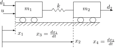
To be more specific, let us analyze the require-ments for the ACC 1992 robust control bench-mark [9]. This system is composed of two masses connected to a single spring (see fig. 2). The out-put variable for this system, y, is the position of
m2, represented byx2,uis the control input act-ing onm1,kis the spring constant; also there are two disturbances, d1 and d2 acting respectively
m1 m2
- k -d2
u
-x1
x2
x3=dxdt1
x4= dxdt2
-d1
Fig. 2. The two-mass-spring system
on m1 andm2. x3 andx4 represent respectively the velocity ofx1andx2.
Assuming that d1 = 0 the transfer function be-tween y(k) andu(k) is
Guy(s) =
k m1m2
s2hs2+k(m1+m2)
m1m2
i (2)
The transfer function betweeny(k) andd2(k) is
Gd2y(s) =
1 m2 s
2+ k m1
s2hs2+k(m1+m2)
m1m2
i (3)
The main requirement for this system is to design a feedback compensator for the 4th-order spring-mass system whose parameters are bounded but unknown. When the 1992 ACC robust control benchmark was presented, four scenarios were proposed. The following constraints correspond to scenario 4:
1. The effort of the controller is limited to |u(k)| less than or equal to 1 (requirement 1 of the previous list).
2. Settling time ts and overshoot Mp are
both minimized. ts is achieved when y(k) is
bounded by±0.1 units (requirement 2 of the pre-vious list).
3. The system is robust with respect to the perturbationsd1 andd2 inm1,m2 and paramet-ric variations ofk. The nominal parameters of the process are:m1=m2=k= 1 (requirement 3 of the previous list).
Requirement 4 of the previous list is needed in the scenario one of the 1992 ACC robust control benchmark. In the rest of the paper it will be assumed that this system has been discretized.
4. The model
This section presents a conceptual design for the requirements document of the 1992 ACC ro-bust control benchmark based on SysML require-ments diagrams and requirerequire-ments tables.
Figure 2. The two-mass-spring system
4 Fernando Valles-Barajas
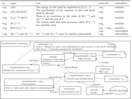
Table 2. Requirements forGc(z−1)
id name text relatesTo relatesHow
req1 u(k) The energy ofu(k) shall be regulated byGc(z−1) req8 satisfy
req2 y(k) andd2(k) shall be allowedThe specification of the response of y(k) and d2(k) req8 satisfy
req3 Gp(z−1) andd There is no restriction in the order of B(z
−1) and
A(z−1) and the size ofd req8 satisfy
req4 B∗(z−1) The system shall deal with processes whichB ∗(z−1)
has unstable zeros req8 satisfy
req8 RSTGc(z−1) req1−req4 satisfy
req9 deriveReq
req9 B(z−1) andA(z−1) B(z−1) andA(z−1) must be coprime polynomials req8 deriveReq
CLOE algorithm req Parametric variations
I Y
y >
verify rationaler3
requirementreq12
Uncorrelated
Text = “y(k) andu(k) must be uncorrelated”
requirementreq5
Parametric variations ofGp(z−
1
)
)
requirementreq11
Closed loop identification
body = “Based on some tests performed on the system, it has been concluded thatGp(z−1) presents parametric variations”
Y
block
Adaptive Controller
tune()
requirementreq10
PEC ofu(k)
CLOE
block
rationaler2 rationaler1
testCase
PEC test
Uncorrelation test
testCase verify
satisfy satisfy
deriveReqt
deriveReqt deriveReqt
refine
Fig. 3. Requirements diagram for parametric variations
Table 2 contains the requirements related to
Gc(z−1). As can be seen in this table, an RST
controller satisfies the requirements 1-4 of the re-quirements specification of the previous section. It can be possible by using an RST controller, to specify the response of the system when a step input is applied in the reference yref(k) or
when the output disturbance d2(k) occurs. An RST controller has the ability to control a pro-cess with a transfer function of any order. Con-trollers like PID lack of this feature [1]. Another disadvantage of a PID controller is that it has some constraints in the relationship between the dead time and the constant time of the process; an RST controller does not have this restriction. The controller design method “tracking and reg-ulation with weighted input”, which is used in the tuning of RST controllers, can deal with pro-cesses that the polynomialB∗(z−1) has unstable zeros. In table 2 a derived requirement from the requirement RST Gc(z−1) was defined, this is a
relationship between A(z−1) and B(z−1) which states that these polynomials must be coprime2. In other words, if ones uses an RST controller
A(z−1) and B(z−1) must be coprime polynomi-als.
Fig. 3 shows a requirements diagram that fo-cuses on requirement 5 which was specified in the previous section. An adaptive controller can deal with time-varying process [1]; this is the rea-son the block Adaptive Controller was chosen to satisfy the requirement parametric variations of
Gp(z−1). This kind of controller was considered
to satisfy one of the requirements for the first scenario of the ACC robust control benchmark: the parameterkis bounded but variable. The ra-tionaler3 justifies the importance of requirement 5. Two requirements are derived from the block 2polynomials A(z−1) and B(z−1) are coprime if
there is not a common factor between them.
F. Valles-Barajas
A SysML requirements model for the 1992 ACC robust control benchmark. 5
Adaptive Controller: PEC of u(k) and Closed loop identification. An adaptive controller iden-tifies the model of the process based on measure-ments of the input u(k) and output y(k) of the process. To get a good model, the content of infor-mation of the signalu(k) must be good enough to find the parameters of Gp(z−1). Formally
speak-ing the signal u(k) must fulfill the Persistent of Excitation Condition (PEC). In what follows the rationale for the PEC is explained; this construct is labeled asr1in the fig. 3.
4.1. Rationale for PEC,r1
Let us represent equation 1 in the difference equation:
y(k+ 1) =−
nA
X
i=1
aiy(k−i) + nB
X
i=1
biu(k−d−i+ 1)
(4) It is desirable to identify the (nA+nB)
param-eters of the model. According to [5], a condi-tion that must be fulfilled in order to achieve this task is that the input variable u(k) has
p-sinusoids components of different frequency (u(k) =Pp
i=1sin(ωiTsk)). If (nA+nB) is even,
then p must be greater than or equal to nA+nB 2 and if (nA+nB) is odd, then pmust be greater
than or equal to nA+nB+1
2 . This condition is known as the Persistent Excitation Condition and is related to the information content of the in-put variableu(k). If the PEC is not fulfilled, the parameters calculated will be either outside the valid zone3or inadmissible.
4.2. Rationale for closed loop identification, r2
As can be seen in fig. 3 the requirement para-metric variations ofGp(z−1) was satisfied by the
blockadaptive controller. This kind of controller performs identification4in closed loop in order to detect any change in the dynamics of the pro-cess and then to update the modelGp(z−1); this
is the reason the requirement closed loop iden-tification was defined as a derived requirement of the block Adaptive Controller. Unfortunately, the performance of an identification in closed loop is decreased when the input of the process u(k), the disturbance d2(k) and noise n(k) (see fig. 1) are correlated and because of this the parameters identified are biased.
3the set of parameters that corresponds to the
pro-cess is called valid zone
4identification is the procedure by which a model of
the process is obtained.
In what follows, a formal explanation of the fun-damental problem of closed-loop identification is given. This explanation is based on [3].
Suppose that the process represented by equation 4 only depends on values ofu(k):
y(k) = B(z−1)u(k) +e(k)
= b1u(k−1) +· · ·+bnu(k−n) +e(k)(5)
wheree(k) represents disturbanced2(k) and noise
n(k) acting on the output y(k). This model can be represented in the following way:
y(k) =φT(k)θ+e(k) (6) where θ = [b1. . . bn]T is the parameter vector of
Gp(z−1) and
φT(k) = [u(k−1). . . u(k−n)]T (7)
is the vector of measurements (y(k) and u(k)), which in this case is composed only by values of
u(k).
Using the least square algorithm to find an esti-mation for the vector θgivenN data points, the next equation is obtained:
ˆ
θ(N) =
"
1
N
N X
k=1
φ(k)φT(k) #−1
1
N
N X
k=1
φ(k)y(k) (8)
= θ+
"
1
N
N X
k=1
φ(k)φT(k) #−1
1
N
N X
k=1 φ(k)e(k)
Under mild conditions on the data set we then have that ˆθ(N) approaches toθ∗with probability 1 where
θ∗ = lim
N→∞E ˆ
θ(N) (9)
= θ+¯
Eφ(k)φT(k)−1 ¯
Eφ(k)e(k) whereExis the mathematical expectation of the random vector xand the “total expectation” op-erator ¯E is defined as
¯
Ex(k) = lim
N→∞ 1
N
N
X
k=1
Ex(k) (10)
The least square algorithm is consistent if ¯
Eφ(k)e(k)≡0 (11) but this is not achieved becauseu(k) ande(k) are correlated due to the fact that the identification
6 Fernando Valles-Barajas
req Uncertainty
i
satisfy
e
y verify
rationale
body = “By observing the forms of the sensitive functions the robustness ofGc(z−
1
) Uncertainty
Text = the system shall be insensitive to uncertainties
requirementreq6
Sensitive functions
testCase
S
testCase
T
testCase
e
Syd1
testCase testCase
U
can be established.”
requirementreq16
Robust controller
˜
Gp(z−
1
)
requirement
req13
n(k)
requirement
req14
d1(k), d2(k)
requirement
req15
Fig. 4. Requirements diagram for the uncertainty in the control system
procedure is carried out in closed loop. This is the reason the derived requirementUncorrelated was defined in fig. 3.
It is important to mention that the algorithm used for identification in an adaptive controller is a recursive version of the Least Square Algo-rithm and it can be shown that the same problem will be presented using this algorithm. The non recursive version of the Least Square Algorithm was used to explain the problem because it is eas-ier to give an explanation of this algorithm. In fig. 3, the closed loop identification require-ment is satisfied by the CLOE block which is an algorithm that performs identification in closed loop [5]. This algorithm is then refined by the use caseCLOE algorithm. TwotestCase blocks were defined in fig. 3:PEC testandUncorrelation test. These blocks will ensure the proper work of the adaptive controller.
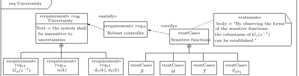
Fig. 4 shows a requirements diagram that fo-cuses in the uncertainty in the control system (requirement 6). To efficiently manage the un-certainty in the system, this requirement was di-vided into three parts by using the composition relation: parametric variations ofGp(z−1),noise
n(k) and external disturbances d1(k) and d2(k). In figure 4, the uncertainty requirement is sat-isfied by a robust controller. To verify the work of this controller atestCase calledsensitive func-tions is defined. The sensitive functions reflect how the system is affected by disturbancesd1(k),
d2(k) and noisen(k). By drawing these functions, a control engineer can determine how robust the system is with respect to these external signals. The output sensitive functionS models the rela-tionship betweeny(k) andd2(k). A measurement of how the output disturbance d2(k) affects the
input u(k) is given by the input sensitive func-tionU. The relationship between noisen(k) and the outputy(k) is known as the complementary sensitive functionT. The last sensitive function,
Syd1(z
−1), establishes a relationship between the disturbanced1(k) and the outputy(k).
In fig. 4 the composition relationship was used to model the relation between the test casesensitive functions and the test cases for each of the sen-sitive functions. It is important to mention that this relationship between test cases is not defined in SysML but the author of this paper believes that a complex test case can be managed more efficiently by using this relationship.
Requirement 7, which reflexes the capacity of the control system to deal with faults, can be satis-fied by using a FDI system which is composed of an isolation and detection block [7].
5. Conclusions
In this paper a novel approach to make a con-ceptual design for the software of control systems has been presented. This approach is based on the notation used in SysML. An example (the 1992 robust control benchmark) to demonstrate the applicability of the approach was given. By using this approach, control engineers can esti-mate the necessary effort to build the software for a control system.
References
[1] K. Astr¨om and K. J. Witternmark.Adaptive Con-trol. Addison-Wesley, USA, 2nd edition, 1995. [2] B. Dutrerte and V. Stavridou. Formal
require-ments analysis of an avionic control system.IEEE Transaction on software engineering, 23(5), 1997.
F. Valles-Barajas
A SysML requirements model for the 1992 ACC robust control benchmark. 7
[3] U. Forssell and L. Ljung.Closed-loop identification revisited.Automatica, 35(7), 1215-1241. 1999. [4] W. S. Humphrey. PSP : A Self-Improvement
Process for Software Engineers. Addison-Wesley, USA, 2005.
[5] I. D. Landau and G. Zito. Digital Control Sys-tems: Design, Identification and Implementation. Springer-Verlag London Ltd, London, 2006. [6] OMG. Systems Modeling Language (SysML)
Specification. Object Management Group, 2006. [7] R. J. Patton, P. M. Frank, and R. N. Clark.
Is-sues of Fault Diagnosis for Dynamic Systems. Springer-Verlag, 2007.
[8] S. Queins, G. Zimmermann, M. Becker, M. Kro-nenburg, C. Peper, R. Merz, and J. Sch¨afer. The light control case study: Problem description.
Journal of Universal Computer Science, 6(7):586– 596, 2000.
[9] W. Reinelt.Robust control of a two-mass-spring system subject to its input constraints.In: Amer-ican Control Conference, 2000.
[10] F. Valles-Barajas A requirements engineering process for control engineering software Innova-tions in Systems and Software Engineering: A NASA Journal, 3(4), 217-227. 2007.
Lietuviˇskas pavadinimas
N1.Surname1, N2.Surname2 Straipsnio santrauka Received February 2009.
A SysML Requirements Model for the 1992 ACC Robust Control Benchmark
A SysML Requirements Model for the 1992 ACC Robust Control Benchmark