The Thirty-Third AAAI Conference on Artificial Intelligence (AAAI-19)
A PAC Framework for Aggregating Agents’ Judgments
Hanrui Zhang
Computer Science DepartmentDuke University Durham, NC 27705 [email protected]
Vincent Conitzer
Computer Science DepartmentDuke University Durham, NC 27705 [email protected]
Abstract
Specifying the objective function that an AI system should pursue can be challenging. Especially when the decisions to be made by the system have a moral component, input from multiple stakeholders is often required. We consider ap-proaches that query them about their judgments in individual examples, and then aggregate these judgments into a general policy. We propose a formal learning-theoretic framework for this setting. We then give general results on how to translate classical results from PAC learning into results in our frame-work. Subsequently, we show that in some settings, better re-sults can be obtained by working directly in our framework. Finally, we discuss how our model can be extended in a vari-ety of ways for future research.
Introduction
As AI systems are being broadly deployed in the world, the problem of specifying theobjective functionsthat they pur-sue is becoming ever more complex. Simple objective func-tions that are sensible for the purpose of evaluating tech-niques in the lab often cause unwanted outcomes in practice. For example, one might try to simply minimize error rate in a speech recognition system, only to realize that the result-ing system performs extremely well on the majority dialect but poorly on the minority dialect. This may socially not be acceptable.
More generally, AI systems increasingly need to make difficult tradeoffs. Should a self-driving car take an action that increases the risk for a nearby pedestrian, but reduces it for the occupant of the car? Should an algorithm that matches patients and donors in a kidney exchange priori-tize younger patients even if this reduces the total number of matches? Given that today’s AI systems do not have a broad understanding of the world, they cannot appropriately make these tradeoffs themselves; human input is required. But these problems are difficult for humans too, and they will not always agree.
One approach to doing so is the following (Conitzer et al. 2017; Noothigattu et al. 2018). Ask multiple human subjects what option they would choose in certain situations in the domain at hand; from this, learn a model for each of them, predicting what they would choose in other situations; and
Copyright c2019, Association for the Advancement of Artificial Intelligence (www.aaai.org). All rights reserved.
then, use techniques fromsocial choicetheory (Brandt et al. 2015) to aggregate this into a single decision policy for the AI system. For example, the “Moral Machine” website de-veloped at MIT invites visitors to consider various scenarios in which the car will necessarily end up killing one group of people (and/or animals) or another, and ask them which they would choose.1 Indeed, these responses have been
ag-gregated into policies via a voting-based approach (Nooth-igattu et al. 2018). In a similar project, MTurkers were asked such comparison queries in the context of kidney exchanges and their responses were aggregated into a policy (Freedman et al. 2018).
Human subject responses are not freely available. They either require compensation (e.g., MTurkers) or a gamified design that makes it enjoyable to participate but may come at other costs.2This raises several related questions for the purpose of designing similar systems. How many responses should we aim to get? Do we need to recruit many distinct subjects, or does it suffice to have many responses from a few subjects? Do random queries suffice or should we actively design them? In this paper, we propose a formal learning-theoretic framework for this problem, building on the framework of Probably Approximately Correct (PAC) learning (Valiant 1984). In our model, there is a single cor-rectconceptc∗ that we attempt to learn.3Each human
sub-jectj has her own conceptcj, which is a noisy estimate of the correct concept. When we ask subjectj queryxj,k, the subject will respond withyj,kaccording to her own concept
cj. From these responses, we aim to learn the correct con-ceptc∗.
1
This project has been much maligned for focusing on an unre-alistic problem. But there is no doubt that self-driving cars will face
someproblems where they will have to make such tradeoffs, for ex-ample in deciding how aggressive to be in merging lanes (Sadigh et al. 2016).
2
The Moral Machine team has been open about prioritizing the site going viral over other objectives.
In the remainder of the paper, we first formally introduce the framework. We then give general results on how to trans-late classical results from PAC learning into results in our framework. Subsequently, we show that in some settings, better results can be obtained by working directly in our framework. Finally, we discuss how our model can be ex-tended in a variety of ways for future research.
Related Work
There is a rich body of research on learning from mul-tiple entities, among which most closely related to ours are collaborative learning(Blum et al. 2017; Qiao 2018),
domain adaptation (Mansour, Mohri, and Rostamizadeh 2009a; 2009b), and learning from nearby sources (Cram-mer, Kearns, and Wortman 2006; 2008). Collaborative learn-ing concerns a settlearn-ing in which multiple agents try to learn the same concept with respect to their own distinct distri-butions of data points; in contrast, in our setting, agents draw data points from the same global distribution, but la-bel based on their own noisy concepts. Domain adaptation concerns a problem in which, given concepts with small er-rors w.r.t. different distributions, the goal is to aggregate the given concepts into a new one, with small error w.r.t. any mixture of the distributions. The setting is intrinsically dif-ferent from ours, in the sense that (1) in our setting, all data points are from the same distribution (but are labeled accord-ing to different noisy concepts), and (2) our goal is to recover the ground truth instead of combining existing slightly er-roneous ones into another slightly erer-roneous one. Learning from nearby sources considers a problem in which, given la-beled data sets w.r.t. different sources and the “similarity” between these sources, the goal is to select a subset of data that will result in the best model for each of the sources. This problem, while being similar to ours in terms of the ex-istence of multiple sources, studies estimation of many po-tentially unrelated concepts, instead of one ground truth.
Another line of work isnoise-tolerant learning(Kearns 1998; Blum, Kalai, and Wasserman 2003; Natarajan et al. 2013). This problem is similar to ours in the sense that the goal is also to learn a target concept with noisy data points. However, in noise-tolerant learning, noise models are usu-ally less structured: normusu-ally, all data points are corrupted in a more or less homogeneous way, at random (e.g., flipping each label independently with a fixed probability) or adver-sarially. Relatedly, Michael (2010) considers PAC learning when part of each data point is hidden, and Blum and Cha-lasani (1992) consider a setting where whenever a data point is labeled, it is labeled according to some concept drawn randomly or adversarially from a fixed set. In our model, in contrast, it is known which data points are from which agent, and each agent labels according to a single concept; the aggregation algorithm can, and should, make use of this information.
Judgment aggregation is a central topic in social choice theory, to which a significant body of research has been devoted (e.g., (Endriss, Grandi, and Porello 2012; Endriss 2016)). There, the problem is how to aggregate diverse judg-ments into a single outcome. In contrast, in this paper, we focus less on pure social-choice-theoretic aspects and more
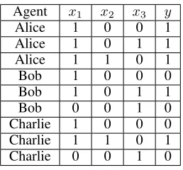
Agent x1 x2 x3 y
Alice 1 0 0 1
Alice 1 0 1 1
Alice 1 1 0 1
Bob 1 0 0 0
Bob 1 0 1 1
Bob 0 0 1 0
Charlie 1 0 0 0
Charlie 1 1 0 1
Charlie 0 0 1 0
Table 1: Reports by the agents.
on statistical learning aspects.
The PAC Judgment Aggregation Model
Before formally introducing our model, first we discuss a concrete example.Example 1. Suppose we want to learn a Boolean conjunc-tion formula from the agents. Each of the3 agents, Alice, Bob, and Charlie, has responded to3queries (see Table 1). Observe that every agent is consistent, in the sense that there is indeed a Boolean conjunction that conforms with her/his reports. In particular, Alice’s formula isx1, Bob’s isx1∧x3, and Charlie’s is eitherx2orx1∧x2. But our goal is to find anaggregateconjunction.
One way to aggregate the responses of the 3 agents is to find the Boolean conjunction that conflicts with as few reports as possible. The resulting aggregate conjunction is
x1, which conflicts only with Bob’s first report and Char-lie’s first report. One may check that any other conjunction conflicts with more data points.
An alternative way of aggregating is to first compute the
majority labelon every feature vector, and then find the for-mula that conflicts with as few of the majority labels as pos-sible. Among the9data points, there are only4distinct fea-ture vectors:(1,0,0),(1,0,1),(1,1,0)and(0,0,1), and the majority judgments on these feature combinations are0,1,
1, and0, respectively. Given these majority labels, there are
4formulas that conflict with only1label:x1,x2,x1∧x2, andx1∧x3. Depending on the tie-breaking rule, any one of these4might be the aggregate formula.
From the above example, we see that the aggregate re-sult depends heavily on the method used. To decide which method is best, we consider the following statistical model of the problem. As described in the introduction, this model assumes that every agent responds to data points (feature vectors) according to her own noisy estimate of the correct concept. Formally:
Definition 1 (PAC Judgment Aggregation). Given a dis-tribution of data points D, a concept class C where each
c ∈ C maps each data point in the support ofDto a label in{−1,1}, and a noisy mappingν : C → ∆(C)4 which
maps each concept to a distribution over concepts, the PAC
4
judgment aggregation problem (with parametersεandδ) is defined as follows:
1. A ground truth conceptc∗∈ Cis chosen.
2. m agents’ concepts, denoted by A = (c1, . . . , cm) are generated by drawing independent and identically dis-tributed (i.i.d.) samples fromν(c∗).
3. ` data points are generated for each agent j, by draw-ing i.i.d. samples(xj,k)
k∈[`]5 and attaching to each sam-ple xj,k the label yj,k = cj(xj,k), together forming
((xj,k, yj,k)) k∈[`].
4. Based on the data points (((xj,k, yj,k))
k∈[`])j∈[m], a learning algorithm computes a hypothesis h ∈ C. We are interested in algorithms that, with probability at least
1−δ, compute a hypothesishthat satisfies:
Pr
x∼D[c
∗(x)6=h(x)]≤ε.
Definition 1 can be viewed as a natural generalization of the PAC learning model in the presence of noise in agents’ judgments. In fact, if the noise vanishes, i.e., if the noisy mapping satisfies that for anyc∈ C,Prcν∼ν(c)[c=cν] = 1,
then with probability1, every agent has the same concept— the ground truth. In this special case, it does not help to query more than1agent, so that PAC aggregation coincides with PAC learning.
In the rest of this paper, we considerfiniteconcept classes, and focus onexact recoveryof the ground truth. That is, we consider algorithms that with probability 1−δoutput the correct concept, h = c∗. This is natural when C is finite:
fixing a distributionD, for anyεsmaller than the minimum probability that two concepts differ, the algorithm must out-put exactly the ground truth with high probability.6
General Algorithms for PAC Aggregation
In this section, we present two paradigms to extend general sample complexity upper bounds from the traditional PAC learning setting to our PAC aggregation setting.Before proceeding to the paradigms, we define the dis-tancebetween two concepts, which helps simplify the nota-tion. The intuition is straightforward: fixing the distribution
Dover data points, the probability that two concepts differ at a random data point induces a metric over the concept class. Formally, for two conceptsc1andc2, we define the distance betweenc1andc2to be
d(c1, c2) = Pr
x∼D[c1(x)6=c2(x)].
One can show thatd(·,·)is indeed a metric overC; in par-ticular, it satisfies the triangle inequality.
With the above definition of distance between concepts, in Definition 1, one may equivalently require the output hypothesis h to satisfy: with probability at least 1 − δ,
d(c∗, h)≤ε. In the rest of the paper, we will use this simpler notation whenever possible.
5[`]
denotes the set{1,2, . . . , `}. 6
We assume that any two distinct concepts differ with positive probability, i.e., the probability of drawing a data point on which they disagree is positive.
Occam’s Razor
Recall the following basic result in PAC learning for when the concept class is finite:
Proposition 1(Occam’s Razor for PAC learning (Folklore)).
WithOlog(|C|ε /δ)data points, a conceptcthat minimizes
empirical error, which by definition is consistent withc∗on all data points, satisfiesd(c, c∗)≤εwith probability at least 1−δ.
For exact recovery, when the minimum gap between any two concepts is α (i.e., minc16=c2d(c1, c2) = α), setting
ε = α/2, Occam’s Razor guarantees that Olog(|C|α/δ)
data points are sufficient to recoverc∗. Note that the num-ber of required data points increases as the size of the con-cept classC increases and the gap αdecreases. In the rest of this subsection, we prove an extension of Occam’s Razor to the PAC aggregation model, with an additional parameter characterizing the dependence on the strength of the noise (which is always0in PAC learning).
Theorem 1 (Occam’s Razor for PAC Aggregation). Sup-pose the noisy mappingνsatisfies the following two condi-tions:
1. For anycandc06=c,
Ecν∼ν(c)[d(c, cν)]≤Ecν∼ν(c)[d(c 0, c
ν)]−αOR.
2. For anyc and c0 (where possibly c = c0), lettingcν ∼ ν(c),d(c0, cν)is sub-Gaussian with parameterβ, i.e., for
anyλ∈R,
E[exp(λ(d(c0, cν)−E[d(c0, cν)]))]≤exp(β2λ2/2).
Then, using m = Olog(|C|α2/δ)β2 OR
agents and `m =
Olog(α|C|2 /δ) OR
data points in total, with probability at least
1−δ, a conceptcthat minimizes the empirical error, defined as
errA,S(c) =
1
`m
X
j∈[m],k∈[`]
I[c(xj,k)6=yj,k],
is the ground truth.
Before proving the theorem, we briefly discuss the impli-cations of its components:
Dependence on αOR. Condition 1 of the theorem states that in expectation, the noisy versioncν of a conceptc is closer to c than to any other concept. The gap αOR by which cν is closer to c than to any other concept deter-mines the number of agents and samples required to re-coverc. The larger the gap is, the fewer agents and sam-ples are required. In particular, when the noise vanishes, for
c,c0 6= c, andcν ∼ ν(c), we havec = cν, and therefore d(c, cν) = d(c, c) = 0, and d(c0, cν) = d(c, c0). In such cases, αOR is the minimum distance between two distinct concepts.
Dependence onβ. Condition 2 of the theorem states that the distribution of noisy judgments is well concentrated, in the sense that the distance between cν and any concept is a sub-Gaussian random variable with parameter β. The smallerβ is, the fewer agents are required. This condition may appear rather strong at first sight. Nevertheless, since
d(c0, cν) ∈ [0,1], it is always true that d(c0, cν) is sub-Gaussian with parameter 1/2 (i.e., β ≤ 1/2). In natural noise models, the sub-Gaussian parameter β goes to 0 as the noise vanishes, in which case the number of agents re-quired is significantly reduced. For example, if the noisy ver-sioncν of c is never too far away fromc—i.e., for any c, cν ∼ν(c), we haved(c, cν) ≤γwith probability1—then we haveβ≤min{γ,1/2}. This is because for anyc0, by the triangle inequalityd(c0, cν)∈[d(c, c0)−d(c, cν), d(c, c0) + d(c, cν)]⊆[d(c, c0)−γ, d(c, c0) +γ], and any random vari-able with a support of length bounded by2γis sub-Gaussian with parameterγ. In particular, when there is no noise (i.e.,
cν = c with probability1), we haveβ = 0, andm = 1 agent suffices7—corresponding to the traditional PAC
learn-ing settlearn-ing.
Tradeoff betweenmand`. Whenβ =o(1), the required number of agentsmis asymptotically smaller than the total number of data points`m. As a result, a tradeoff betweenm
and`emerges: while keeping the probability of failureδthe same, one may use more data points per agent in order to de-crease the number of agents needed (and vice versa), as long as the number of agents meets the minimum requirement.
Learnability with` = 1data point per agent. Setting
β= 1/2in the second condition of Theorem 1, we immedi-ately obtain the following simpler version:
Corollary 1 (Occam’s Razor, Simplified). Suppose the noisy mappingνsatisfies: for anycandc06=c,
Ecν∼ν(c)[d(c, cν)]≤Ecν∼ν(c)[d(c 0, c
ν)]−αOR,
Then, usingm=Olog(α|C|2 /δ) OR
agents and`= 1data point
per agent, with probability1−δ, a concept that minimizes the empirical error is the ground truth.
In other words, with sufficiently many agents, one data point per agent suffices to recover the ground truth.
7
Here, we abuse notation to allow1 =O(0).
Computational efficiency. Like the classical Occam’s Razor result for PAC learning, Theorem 1 does not guaran-tee computational efficiency. This is because it is sometimes hard to compute a minimizer of the empirical error. Indeed, it is impossible to design general algorithms for PAC learn-ing/aggregation that are “computationally efficient” without specifying the representation of the particular problem. In a later section, we present computationally efficient algo-rithms in several specific settings. We now turn back to prove Theorem 1.
Proof of Theorem 1. First we define some notation. Recall that A = (c1, . . . , cm) is the (ordered) set of agents. Let
S= ((xj,k)
k)jbe the (ordered) set of data points. Let
errA(c) =ES∼D`m[errA,S(c)]
err(c) =EA∼(ν(c∗))m[errA(c)].
denote the expected empirical error of a conceptc, with the latter expression also taking the expectation over the agents’ concepts. For eachc ∈ C, we show that with high probabil-ity, the empirical error ofcis close to its expectation. Fixing
c, consider two events:
• E1:|errA,S(c)−errA(c)| ≤ 16αOR.
• E2:|errA(c)−err(c)| ≤ 16αOR.
We show that both events happen with high probability, so with high probability they happen simultaneously, in which case we have:
|errA,S(c)−err(c)| ≤
1 3αOR.
First we bound the probability that E1 does not hap-pen. Note that conditioned on A, errA,S(c) is the aver-age of`mindependent r.v.’s in[0,1], namely{I[c(xj,k) =
yj,k]}j,k, with meanerrA(c). Applying the Hoeffding bound toerrA,S(c)conditioned onA, we have
Pr
|errA,S(c)−errA(c)|>
1 6αOR
≤2e−`mα2OR/18≤ δ
2|C|.
Now considerE2. Observe thaterrA(c) = m1 Pjd(c, c j)
anderr(c) =Ecν∼ν(c∗)[d(c, cν)]. It follows thaterrA(c)is
sub-Gaussian with parameter √β
m. Applying the Hoeffding bound for sub-Gaussian variables toerrA(c)gives
Pr
|errA(c)−err(c)|>
1 6αOR
≤2e−mα2OR/72β2≤ δ
2|C|.
Now taking the union bound over the two events and all concepts, with probability1−δ, for anyc∈ C,
|errA,S(c)−err(c)| ≤
1 3αOR.
In that case, for anyc6=c∗, we have
errA,S(c∗)≤err(c∗) +
1
3αOR≤err(c)− 2 3αOR
≤errA,S(c)−
1
3αOR<errA,S(c).
Majority Voting
When the support ofD, denoted by |D|, is finite, another way to aggregate agents’ judgments is to first estimate their individual concepts, and then let these estimated concepts take a majority vote for eachxin the support ofD(denoted byx∈ D). Formally, we have:
Theorem 2. When|D|is finite, if
1. the minimum distance between concepts isαMV>0, and
2. the noisy mapping satisfies, for someθ >0, that for any
x∈ D,Prcν∼ν(c)[c(x) =cν(x)]≥ 1 2+θ,
then with m = Olog(|D|θ2/δ)
agents and ` =
Olog(|C|αlog|D|/θδ)
MV
data points per agent, the pointwise
majority concepthof the empirical error minimizershj of
each agent’s data points, i.e., the concepthsuch that for any
x ∈ D,h(x) = sgnP
jh
j(x), is the ground truth with
probability1−δ.
Again, before proceeding to the proof, we discuss the im-plications of the various components of the theorem.
Dependence on|C|. As in the Occam’s Razor result, the number of data points required by the majority-voting ap-proach depends logarithmically on|C|. However, unlike in Occam’s Razor, the number of agents required for majority voting does not explicitly depend on |C|. This can be par-tially explained by the fact that since|D|<∞, there are at most2|D|possible concepts in total.
Dependence on|D|. Although, in contrast to Occam’s Ra-zor, majority voting requiresDto be finite, one may observe that the dependence on|D|is rather mild, i.e., logarithmic for m and doubly logarithmic for `. This means majority voting remains relatively efficient even when|D|grows ex-ponentially fast.
Dependence onαMV. The parameterαMVhere is similar toαORin Occam’s Razor, in the sense that when the noise vanishes, i.e.,Prcν∼ν(c)[cν = c] = 1, the two parameters
are exactly the same. The key difference is that, for majority voting,αMVdoes not depend on the strength or form of the noise.
Dependence onθ. Majority voting requires that the noisy concepts are more likely to agree with the ground truth. The parameter θ can be viewed as the distance between the expected judgment and a random guess, which in some sense characterizes the strength of the noise. The largerθis, the easier to distinguish the noisy judgments from random guesses and extract the ground truth, and therefore fewer agents and data points are required.
Now we prove Theorem 2.
Proof of Theorem 2. We first show that with probability
1− δ
2, the empirical error minimizers for the agents’ data
points coincide exactly with the agents’ concepts.
Ac-cording to Proposition 1, with ` = Olog(α|C|m/δ)
MV
=
Olog(|C|αlog|D|/θδ)
MV
data points,hj =cjwith probability
at least1− δ
2m. Taking the union bound over themagents, we conclude that with probability at least1−δ
2, it is the case that for everyj,hj=cj.
Now, conditioning on the event thathj = cj for anyj, we show that majority voting recoversc∗exactly with prob-ability at least1−δ
2. Consider somex∈ Dwhere w.l.o.g.
c∗(x) = 1. SincePrcj∼ν(c∗)[cj(x) = 1]≥1
2+θ, the Cher-noff bound gives
Pr
1
m
X
j∈[m]
hj(x)≤0
≤exp(−θ2m/2).
With m = Olog(|D|θ2 /δ)
, the right hand side is at most δ
2|D|. Taking the union bound over the support of D, we
have: with probability1−δ
2, for allx∈ D,h(x) =c
∗(x).
Recall that the immediately preceding argument condi-tioned onhj =cjfor allj, which happens with probability at least1−δ
2. Taking the union bound over the two parts, it follows that with probability at least1−δ, the pointwise majority concepthis exactly the ground truthc∗.
Finally, we note that the definition of the pointwise ma-jority concept does not guarantee its membership inC. This is not a problem, because when the algorithm succeeds, we do haveh∈ Csincec∗∈ C. When it fails andh /∈ C, we can let the algorithm output an arbitrary hypothesis inC.
Occam’s Razor vs. Majority Voting
Occam’s Razor (Theorem 1) and majority voting (Theo-rem 2) rely on different parameters. As these parameters vary across settings, either approach may be preferred over the other. Two key differences are:
1. Theorem 2 requires both|D| and|C|to be finite, while Theorem 1 depends only on|C|. This means majority vot-ing may fail when the support ofDis infinite.
2. The parameterαMVin Theorem 2 is always positive, but Theorem 1 puts a strong requirement on the gapαORthat in principle does not always hold. As an extreme (if un-realistic) example, suppose that the noisy mapping ν is actually a deterministic permutation of the concept space
C. In this case, the noisy version of a concept is clearly closer in expectation to another concept, namely the con-cept to which it is deterministically mapped.
Tighter Bounds in Restricted Settings
In this section, we consider a linear model, where each con-ceptcis ann-dimensional vector inRn. For a data pointx(also in Rn), the label thatcassigns toxis determined by the sign ofc·x, denoted bysgn(c·x).8
8
For simplicity, we consider only D such that for any c,
ALGORITHM 1:Aggregation algorithm for binary judgments.
Input :`labeled samples each frommagents{(xj,k, yj,k)}j,k.
Output:hwhich with high probability is equal toc∗.
fori∈[n]do
Lethi←sgnP j,ksgn
xj,ki yj,k
end
Outputh= (hi)i
One example of the linear model is pass/fail exams in which there arentrue-or-false questions. If conceptc∗is the ground truth solution, then the correct answer to questioniis
sgn(c∗i)and that question is worth|c∗i|points, i.e., the right answer to thei-th question increases the score by|c∗i|, and the wrong one decreases the score by|c∗i|. The support of
Dis{−1,1}n, wherex ∈ D corresponds to a completed exam with a true or false (1 or −1) answer to every ques-tion. Hence, indeed, thecorrectscore for completed examx
isc∗·x. A completed exam should get a grade of “Pass” if
c∗·x >0and “Fail” otherwise. Unfortunately, there are only imperfect evaluators—themjudges—available to grade the exams, where judgej’s estimate of the ground truth iscj. Thus, when judgejevaluates an exam,jwill output “Pass” if and only ifcj·x >0. Each judgejmakes P/F decisions about`sampled completed exams{xj,k}
k∈[`]. Given these samples and labels, our aim is to recover the ground truthc∗.
(In real applications, an “exam” can be any test with a vector of binary outcomes, and a “judge” any individual that makes judgments about what the overall result should be.)
We show that in certain settings, while the general Oc-cam’s Razor (Theorem 1 and Corollary 1) and majority vot-ing (Theorem 2) results yield nontrivial sample complexity bounds, both the required number of agentsmand the total number of data points`m can be significantly reduced us-ing settus-ing-specific methods. We further prove nearly tight lower bounds onmand`m.
Efficient Learning Algorithms
We give efficient algorithms for two restricted settings in the linear model. First, we consider the following setting: the at-tributes of instances are i.i.d., agents only make binary (pos-itive/negative) judgments about (i.e., place binary weights on) each attribute, and each agent’s judgment about an at-tributecji is obtained independently by flipping the corre-sponding judgment in the ground truth,c∗i, with some fixed probability. We show that as long as the distribution of the at-tributes is not extremely heavy-tailed and the noisy mapping preserves some information about the ground truth, then we can efficiently recover the ground truth. Formally, we prove the following theorem:
Theorem 3(Binary Judgments, I.I.D. Symmetric Distribu-tions). Suppose that C = {−1,1}n; for each i ∈ [n],
Di =D0is a non-degenerate9symmetric distribution with
bounded absolute third moment; and the noisy mapping with
9D
is non-degenerate if forX∼ D,Pr[X= 0]6= 1.
noise rateηsatisfies
ν(c)i =
( c
i, w.p.1−η
−1, w.p.η/2 1, w.p.η/2
,
Then, Algorithm 1 withm=Oln((1−n/δη)2)
agents and`m=
On(1ln(−n/δη)2)
data points in total outputs the correct
con-cepth=c∗with probability at least1−δ, inO(`mn)time.
The proof of Theorem 3, as well as those of Propositions 2 and 3 and Theorems 4, 5 and 6, are available in the appendix of the full version of the paper. To demonstrate the power of setting-specific algorithms, we compare Theorem 3 with the guarantees provided by Theorems 1 and 2.
Performance of Occam’s Razor. Recall that the bounds of Theorem 1 rely on 3 parameters:|C|,αORandβ. When
C={−1,1}n,|C|= 2n, and one may show:
Proposition 2. WhenCandνsatisfy the conditions in The-orem 3, andDis the uniform distribution over{−1,1}n, we
haveαOR= Θ 1
−η
√
n
.
So, applying Theorem 1 to the above setting, we obtain
that with`m = On2(1log(1−η)/δ2 )
data points (andm ≤ `m
agents10), the empirical error minimizer is the ground truth with probability1−δ. That is, even with the further restric-tion that the distriburestric-tionDis uniform, this number is larger roughly by a factor ofnthan the corresponding requirement of Theorem 3.
Performance of majority voting. Now we consider The-orem 2. The parameters involved are|C| = 2n,|D| = 2n,
αMVandθ. One may show:
Proposition 3. WhenCandνsatisfy the conditions in The-orem 3, andDis the uniform distribution over{−1,1}n, we
haveαMV= Θ(n−1/2)andθ= Θ 1
−η
√
n
.
So, applying Theorem 2, majority voting requiresm =
On2(1log(1−η)/δ2 )
agents and `m = On7/2log((1−n/η)(12−η)δ)
data points in total. The number of agents required is at least the same as that of Occam’s Razor, and the number of data points is even larger than that of Occam’s Razor by a factor of n3/2. To summarize, for the setting above, the setting-specific algorithm outperforms the general ones, and Occam’s Razor outperforms majority voting.
We now proceed to an efficient algorithm for another set-ting, where the distributions of the attributes are independent (but not necessarily identical) Gaussian distributions, agents have discrete (instead of binary) judgments about each at-tribute, and the noisy mapping flips the sign of the judgment of the attribute independently with some fixed probability. In
10
ALGORITHM 2:Aggregation algorithm for discrete judgments.
Input :`labeled samples each frommagents{(xj,k, yj,k)}j,k.
Output:hwhich with high probability is equal toc∗.
fori∈[n]do
Lets2i ←`m1 P
j,k(x j,k
)2
Letai← 1
si
1
`m P
j,ksgn
xj,ki
yj,k
end
Leta0←miniai
fori∈[n]do
Lethi=pi/qibe the closest fraction toai/a0, where
pi, qi∈Z∩[−d, d]andpi>0.
end
Outputh= (hi)i
words, at the cost of further restricting the shape of the distri-butionD, this setting allows more heterogeneity across the attributes, in the sense that the sizes of both the attributes’ values and the judgments can vary. Formally, we prove:
Theorem 4 (Discrete Judgments, Independent Gaussian Distributions). For constant d, suppose that C = (Z ∩ [−d, d])n; for eachi ∈ [n],D
i = N(0, σ2i)is a Gaussian
distribution with mean0and standard deviationσi∈[1, d];
and the noisy mapping with noise rateηsatisfies
ν(c)i=
( c
i, w.p.1−η
−|ci|, w.p.η/2
|ci|, w.p.η/2 ,
Then, Algorithm 2 withm=Oln((1−n/δη)2)
agents and`m=
On(1ln(−n/δη)2)
data points in total outputs a correct concept
h, in the sense that there is someα∈R+such thath=αc∗, with probability at least1−δ, inO(`mn)time.
Lower Bounds
Now that we have provided some efficient algorithms, we discuss the information-theoretic hardness of the linear model. We show that, even in highly restricted settings, the numbers of agents and data points required to recover the ground truth are roughly the same as the upper bounds ob-tained in Theorems 3 and 4.
In our first lower bound, we restrict attention to binary judgments. We show that even if the algorithm is given each agentj’s exact conceptcj—which is the most it could hope to learn for any number`of samples per agent—it still needs
Ωlog((1−n/δη)2)
agents to recover the ground truth. Formally:
Theorem 5 (Lower Bound: Number of Agents). If C =
{−1,1}n and D
i is the uniform distribution over{−1,1},
then any algorithm that outputs the correct concept with
probability1−δrequiresm= Ωlog((1−n/δη)2)
agents.
We note that this lower bound extends immediately to the discrete-judgments setting in Theorem 4. It follows that the requirement on the number of agents in Theorems 3 and 4
(i.e.,m=Olog((1−n/δη)2)
) is tight up to a constant factor.
Next, we prove a lower bound on the total number of data points (or agents) when each agent reports only1data point.
Theorem 6(Lower Bound: Total Number of Data Points).
IfC={−1,1}n,D
iis the uniform distribution over{−1,1}
or the standard Gaussian distributionN(0,1), the number of data points per agent is` = 1, and1−η = Ω(n−1/2),
then any algorithm that outputs the correct concept with
constant probability requires`m= Ω(1−nη)2
data points in total.
Given Theorem 6, the requirement in Theorems 3 and 4 (i.e., `m = On(1log(−ηn/δ)2)
) is tight up to a factor of
log(n/δ), when ` = 1. We suspect that the loss of the
log(n/δ)factor is due to an intrinsic limitation of the mu-tual information argument used to prove the theorem.
Discussion
Our objective in this paper has been to introduce a general framework for learning from multiple agents’ judgments, and to illustrate the types of results that can be obtained in this framework. Much work remains to be done.
While we have provided some results that are quite gen-eral, we have also shown that sometimes stronger results can be obtained for more specific settings, with specific assump-tions on the distribution of instances, concept class, and noise in the agents’ perceived concepts. This raises the ques-tion of whether similar results can be obtained under differ-ent assumptions that may fit particular applications better. It should be noted that in many cases, an efficient PAC aggre-gation algorithm also implies an efficient algorithm in the simpler traditional PAC learning model for the same con-cept class. However, PAC learning of some natural concon-cept classes is known to be computationally hard. For example, efficient PAC learning algorithms for 3-term DNFs do not exist unlessRP =NP(see (Kearns, Vazirani, and Vazirani 1994)); hence, the same is true for efficient PAC aggregation algorithms in this setting.
A natural variant would allowactive learning, where in-stead of receiving the labels for random instances, the al-gorithm can choose which instances it would like to have labeled (and by which agents).11Indeed, if we consider
set-tings such as that of the MIT Moral Machine, this is po-tentially a sensible model, because those who designed the website control which instances are shown. It would thus be desirable to extend the theory of active learning to this set-ting. For example, the majority voting paradigm, which we use to translate passive learning algorithms to our setting, works for active learning too. One may show:
Theorem 7 (informal). Given a PAC active learning al-gorithm for concept classC, under distribution Dof data points, where |C| and |D| are finite and the conditions in Theorem 2 are satisfied, with sufficiently many agents and data points, the algorithm that (1) runs the PAC active learn-ing algorithm on each individual agent’s data points, and
11
then (2) outputs the concept that is the the pointwise ma-jority of the concepts learned in the first step, recovers the ground truth with high probability.
One downside of the active learning approach in this con-text is that the precise instances shown would depend on (for example) the concept class, so that one could not simply re-use the same data for a different concept class. If gathering data from human subjects is costly (in terms of both finances and effort), then using random instances would allow for better re-use (also by other researchers) of the data. Also, of course any upper bound in the passive model still applies in the active model.
One could imagine other modes of interaction yet. For ex-ample, we may show an instance to three agents and ask them to come to a consensus judgment (cf. (Goel and Lee 2016; Fain et al. 2017)). The space of possible designs is extremely broad, and there is much potential for both theo-retical and empirical work.
Acknowledgements
We are thankful for support from NSF under awards IIS-1814056 and IIS-1527434. We also thank anonymous re-viewers for helpful comments.
References
Blum, A., and Chalasani, P. 1992. Learning switching con-cepts. InProceedings of the fifth annual workshop on Com-putational learning theory, 231–242. ACM.
Blum, A.; Haghtalab, N.; Procaccia, A. D.; and Qiao, M. 2017. Collaborative pac learning. InAdvances in Neural Information Processing Systems, 2392–2401.
Blum, A.; Kalai, A.; and Wasserman, H. 2003. Noise-tolerant learning, the parity problem, and the statistical query model.Journal of the ACM (JACM)50(4):506–519.
Brandt, F.; Conitzer, V.; Endriss, U.; Lang, J.; and Procaccia, A. D. 2015. Handbook of Computational Social Choice. Cambridge University Press.
Conitzer, V.; Sinnott-Armstrong, W.; Borg, J. S.; Deng, Y.; and Kramer, M. 2017. Moral decision making frameworks for artificial intelligence. InProceedings of the Thirty-First AAAI Conference on Artificial Intelligence, 4831–4835.
Crammer, K.; Kearns, M.; and Wortman, J. 2006. Learning from data of variable quality. InAdvances in Neural Infor-mation Processing Systems, 219–226.
Crammer, K.; Kearns, M.; and Wortman, J. 2008. Learn-ing from multiple sources. Journal of Machine Learning Research9(Aug):1757–1774.
Elkind, E., and Slinko, A. 2015. Rationalizations of voting rules. In Brandt, F.; Conitzer, V.; Endriss, U.; Lang, J.; and Procaccia, A. D., eds.,Handbook of Computational Social Choice. Cambridge University Press. chapter 8.
Endriss, U.; Grandi, U.; and Porello, D. 2012. Complexity of judgment aggregation. Journal of Artificial Intelligence Research45:481–514.
Endriss, U. 2016. Judgment aggregation. In F. Brandt, V. Conitzer, U. E. J. L., and Procaccia, A., eds.,Handbook of Computational Social Choice. Cambridge University Press. Fain, B.; Goel, A.; Munagala, K.; and Sakshuwong, S. 2017. Sequential deliberation for social choice. InProceedings of the Thirteenth Conference on Web and Internet Economics (WINE-17), 177–190.
Freedman, R.; Borg, J. S.; Sinnott-Armstrong, W.; Dicker-son, J. P.; and Conitzer, V. 2018. Adapting a kidney ex-change algorithm to align with human values. In Proceed-ings of the Thirty-Second AAAI Conference on Artificial In-telligence.
Goel, A., and Lee, D. T. 2016. Towards large-scale deliber-ative decision-making: Small groups and the importance of triads. InProceedings of the Seventeenth ACM Conference on Economics and Computation (EC), 287–303.
Kearns, M. J.; Vazirani, U. V.; and Vazirani, U. 1994. An introduction to computational learning theory. MIT press. Kearns, M. 1998. Efficient noise-tolerant learning from statistical queries. Journal of the ACM (JACM)45(6):983– 1006.
Mansour, Y.; Mohri, M.; and Rostamizadeh, A. 2009a. Do-main adaptation: Learning bounds and algorithms. In22nd Conference on Learning Theory, COLT 2009.
Mansour, Y.; Mohri, M.; and Rostamizadeh, A. 2009b. Do-main adaptation with multiple sources. InAdvances in neu-ral information processing systems, 1041–1048.
Michael, L. 2010. Partial observability and learnability. Ar-tificial Intelligence174(11):639–669.
Natarajan, N.; Dhillon, I. S.; Ravikumar, P. K.; and Tewari, A. 2013. Learning with noisy labels. InAdvances in neural information processing systems, 1196–1204.
Noothigattu, R.; Gaikwad, S. N. S.; Awad, E.; D’Souza, S.; Rahwan, I.; Ravikumar, P.; and Procaccia, A. D. 2018. A voting-based system for ethical decision making. In Pro-ceedings of the Thirty-Second AAAI Conference on Artificial Intelligence.
Qiao, M. 2018. Do outliers ruin collaboration? arXiv preprint arXiv:1805.04720.