S U R V E Y
Open Access
Adversarial attack and defense in
reinforcement learning-from AI security view
Tong Chen
, Jiqiang Liu, Yingxiao Xiang, Wenjia Niu
*, Endong Tong and Zhen Han
Abstract
Reinforcement learning is a core technology for modern artificial intelligence, and it has become a workhorse for AI applications ranging fromAtrai GametoConnected and Automated Vehicle System(CAV). Therefore, a reliable RL system is the foundation for the security critical applications in AI, which has attracted a concern that is more critical than ever. However, recent studies discover that the interesting attack modeadversarial attackalso be effective when targeting neural network policies in the context of reinforcement learning, which has inspired innovative researches in this direction. Hence, in this paper, we give the very first attempt to conduct a comprehensive survey on adversarial attacks in reinforcement learning under AI security. Moreover, we give briefly introduction on the most representative defense technologies against existing adversarial attacks.
Keywords: Reinforcement learning, Artificial intelligence, Security, Adversarial attack, Adversarial example, Defense
Introduction
Artificial intelligence (AI) is providing major break-throughs in solving the problems that have withstood many attempts of natural language understanding, speech recognition, image understanding and so on. The latest studies (He et al. 2016) show that the correct rate of image understanding can reach 95% under certain condi-tions, meanwhile the success rate of speech recognition can reach 97% (Xiong et al.2016).
Reinforcement learning (RL) is one of the main tech-niques that can realize artificial intelligence (AI), which is currently being used to decipher hard scientific problems at an unprecedented scale.
To summarized, the researches of reinforcement learn-ing under artificial intelligence are mainly focused on the following fields.In terms of autonomous driving
(Shalev-Shwartz et al. 2016; Ohn-Bar and Trivedi 2016), Shai
et al. applied deep reinforcement learning to the problem of forming long term driving strategies (Shalev-Shwartz et al.2016), and solved two major challenges in self driv-ing.In the aspect of game play(Liang et al.2016), Silver
et al. (2016) introduced a new approach to computer
Go which can evaluate board positions, and select the
*Correspondence:[email protected]
Beijing Key Laboratory of Security and Privacy in Intelligent Transportation, Beijing Jiaotong University, Beijing, China
best moves with reinforcement learning from games of self-play. Meanwhile, for Atari game, Mnih et al. (2013) presented the first deep learning model to learn con-trol policies directly from high-dimensional sensory input using reinforcement learning. Moreover, Liang et al. (Guo et al.2014) also built a better real-time Atrai game play-ing agent with DQN.In the field of control system, Zhang
et al. (2018) proposed a novel load shedding scheme
against voltage instability with deep reinforcement learn-ing(DRL). Bougiouklis et al. (2018) presented a system for calculating the optimum velocities and the trajectories of an electric vehicle for a specific route. In addition,in the domain of robot application(Goodall and El-Sheimy2017; Martínez-Tenor et al.2018), Zhu et al. (2017) applied their model to the task of target-driven visual navigation. Yang et al. (Yang et al.2018) presented a soft artificial muscle driven robot mimicking cuttlefish with a fully integrated on-board system.
In addition, reinforcement learning is also an
impor-tant technique for Connected and Automated Vehicle
System(CAV), which is a hotspot issue in recent years. Meanwhile, the security research for this direction has attracted numerous concerns(Chen et al.2018a; Jia et al. 2017). Chen et al. performed the first security analysis on the next-generation Connected Vehicle (CV) based transportation systems, and pointed out the current sig-nal control algorithm design and implementation choices
are highly vulnerable to data spoofing attacks from even a single attack vehicle. Therefore, how to build a reliable and security reinforcement learning system to support the security critical applications in AI, has become a concern which is more critical than ever.
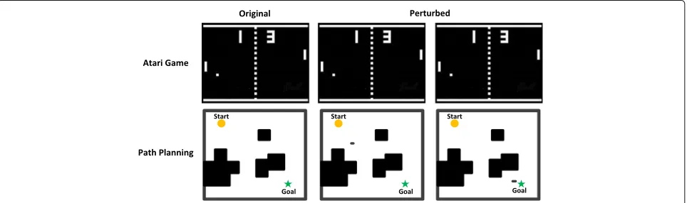
However, the weaknesses of reinforcement learning are gradually exposed which can be exploited by attackers. Huang et al. (2017) firstly discovered that neural network policies in the context of reinforcement learning are vul-nerable to “Adversarial Attacks” in the form of adding tiny perturbations to inputs which can lead a model to give wrong results. Regardless of the learned task or training algorithm, they observed a significant drop in perfor-mance, even with very small adversarial perturbations which are invisible to human. Even worse, they found that the cross-dataset transferability property (Szegedy et al. 2013 proposed in 2013) also holds in reinforce-ment learning applications, so long as both policies have been trained to solve the same task. Such discoveries have attracted public interests in the research of adversarial attacks and their corresponding defense technologies in the context of reinforcement learning.
After Huang et al. (2017), a lot of works have focused on the issue of adversarial attack in the field of reinforce-ment learning (e.g., Fig. 1). For instance, in the field of Atari game, Lin et al. (2017) proposed a “strategically-timed attack” whose adversarial example at each time step is computed independently of the adversarial exam-ples at other time steps, instead of attacking a deep RL agent at every time step (see “Black-box attack” section). Moreover,in the terms of automatic path planning, Liu et al. (2017), Xiang et al. (2018), Bai et al. (2018) and Chen et al. (2018b) all proposed methods which can take adversarial attack on reinforcement learning algorithms
(VIN (Tamar et al.2016), Q-Learning (Watkins and Dayan 1992), DQN (Mnih et al.2013), A3C (Mnih et al.2016)) under automatic path planning tasks (see “Defense tech-nology against adversarial attack” section).
In view of the extensive and valuable applications of the reinforcement learning in modern artificial intelligence (AI), and the critical role for reinforcement learning in AI security, inspiring innovative researches in the field of adversarial research.
The main contributions of this paper can be concluded as follows:
1 We give the very first attempt to conduct a comprehensive and in-depth survey on the literatures of adversarial research in the context of reinforcement learning from AI security view. 2 We make a comparative analysis for the
characteristics of adversarial attack mechanisms and defense technologies respectively, to compare the specific scenarios and advantages/disadvantages of the existing methods, in addition, give a prospect for the future work direction.
The structure of this paper is organized as follow. In “Preliminaries” section, we first give a description for the common term related to adversarial attack under reinforcement learning, and briefly introduce the most representative RL algorithms. “Adversarial attack in rein-forcement learning” section reviews the related research of adversarial attack in the context of reinforcement learn-ing. For the defense technologies against adversarial attack in the context of reinforcement learning are discussed in “Defense technology against adversarial attack” section. Finally, we draw conclusion and discussion in “Conclusion and discussion” section.
Preliminaries
In this section, we give explanation for the common terms related to adversarial attack in the field of reinforce-ment learning. In addition, we also briefly introduce the most representative reinforcement learning algorithms,
and take comparison of these algorithms fromapproach
type, learning type, and application scenarios. So as to facilitate readers’ understanding of the content for the following sections.
Common terms definitions
• Reinforcement Learning: is an important branch of machine learning, which contains two basic elements state and action. Performing a certain action under the certain state, what the agent need to do is to continuously explore and learn, so as to obtain a good strategy.
• Adversarial Example: Deceiving AI system which can lead them make mistakes. The general form of adversarial examples is the information carrier (such as image, voice or txt) with small perturbations added, which can remain imperceptible to human vision system.
1 Implicit Adversarial Example: is a modified version of clean information carrier, which generated by adding human invisible
perturbations to the global information on pixel level to confuse/fool a machine learning technique. 2 Dominant Adversarial Example: is a modified
version of clean map, which generated by adding physical-level obstacles to change the local information to confuse/fool A3C path finding.
• Adversarial Attack: Attacking on artificial intelligence (AI) system by utilizing adversarial examples. Adversarial attacks are generally can be classified into two categories:
1 Misclassification attacks: aiming for generating adversarial examples which can be misclassified by target network.
2 Targeted attacks: aiming for generating adversarial examples which can target
misclassifies into an arbitrary label designated by adversary specially.
• Perturbation: The noise added on the original clean information carriers (such as image, voice or txt), which can make them to be adversarial examples.
• Adversary: The agent who attack AI system with adversarial examples. However, in some cases, it also refer to adversarial example itself (Akhtar and Mian
2018).
• Black-Box Attack: The attacker has no idea of the details related to training algorithm and
corresponding parameters of the model. However, the attacker can still interact with the model system, for instance, by passing in arbitrary input to observe changes in output, so as to achieve the purpose of attack. In some work (Huang et al.2017), for black-box attack, authors assume that the adversary has access to the training environment (e.g., the simulator) but not the random initialization of the target policy, and additionally may not know what the learning algorithm is.
• White-Box Attack: The attacker has access to the details related to training algorithm and
corresponding parameters of the model. Attacker can interact with the target model in the process of generating adversarial attack data.
• Threat Model: Finding system potential threat to establish an adversarial policy, so as to achieve the establishment of a secure system (Swiderski and Snyder2004). In the context of adversarial research, threat model considers adversaries capable of introducing small perturbations to the raw input of the policy.
• Transferability: an adversarial example designed to be misclassified by one model is often misclassified by other models trained to solve the same task (Szegedy et al.2013).
• Target Agent: The target subject attacked by adversarial examples, usually can be a network model trained by reinforcement learning policy, which can detect whether adversarial examples can attack successfully.
Representative reinforcement learning algorithms
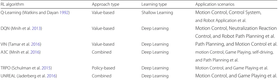
In this section, we list the most representative reinforce-ment learning algorithms, and make comparison among them which can be shown in Table1, where “value-based” denotes that the reinforcement learning algorithm cal-culates the expected reward of actions under potential rewards, and takes it as the basis for selecting actions. Meanwhile, the learning strategy for “value-based” rein-forcement learning is constant, in other words, under the certain state the action will be fixed.
While the “policy-based” represented that the reinforce-ment learning algorithm trains a probability distribution by strategy sampling, and enhances the probability of selecting actions with high reward value. This kind of rein-forcement learning algorithm will learn different strate-gies, in other words, the probability of taking one action under the certain state is constantly adjusted.
• Q-Learning
Table 1The comparison of the most representation reinforcement learning algorithms
RL algorithm Approach type Learning type Application scenarios
Q-Learning (Watkins and Dayan1992) Value-based Shallow Learning Motion Control, Control System,
and Robot Application et al.
DQN (Mnih et al.2013) Value-based Deep Learning Motion Control, Neutralization Reaction Control, and Robot Path Planning et al.
VIN (Tamar et al.2016) Value-based Deep Learning Path Planning, and Motion Control et al.
A3C (Mnih et al.2016) Combined Deep Learning motion Control, Game Playing, self-driving,
and Path Planning et al.
TRPO (Schulman et al.2015) Policy-based Deep Learning Motion Control, and Game Playing et al.
UNREAL (Jaderberg et al.2016) Combined Deep Learning Motion Control, and Game Playing et al.
Approach Typecontains two categories, namelyPolicy-based, andValue-based. Meanwhile,learning Typealso contains two categories, namelyShallow Learning, andDeep Learning
Q-Learning was firstly proposed by C.Watkins (Watkins and Dayan 1992) in his Doctoral Dissertation Learning from delayed rewards in 1989. It is actually a variant of Markov Decision Process (MDP)(Markov1907). The idea of Q-Learning is based on the value iteration, which can be concluded as, the agent perceives surrounding infor-mation from the environment and selects appropriate methods to change the sate of environment according to its own method, and obtains corresponding incen-tives and penalties to correct the strategy. Q-Learning proposes a method to update the Q-value, which can be concluded as Q(St,At) ← Q(St,At) + α(Rt+1 + λmaxaQ(St+1,a) − Q(St,At)). Throughout the contin-uous iteration and learning process, the agent tries to maximize the rewards it receives and finds the best path to the goal, and the Q matrix can be obtained. Q is an action utility function that evaluates the strengths and weakness of actions in a particular state and can be interpreted as the brain of an intelligent agent.
• Deep Q-Network (DQN)
DQN is the first deep enhancement learning algorithm proposed by Google DeepMing in 2013 (Mnih et al.2013) and further improved in 2015 (Mnih et al. 2015). Deep-Mind applies DQN to Atari games, which is different from the previous practice, utilizing the video informa-tion as input and playing games against humans. In this paper, authors gave the very first attempt to introduce
the concept of Deep Reinforcement Learning, and has
attracted public attentions in this direction. For DQN, as the output for the value network is the Q-value, then if the target Q-value can be constructed, the loss function
can be obtained byMean-Square Error (MSE). However,
the input for value network are state S, action A, and feedback rewardR. Therefore, how to calculate the tar-get Q-value correctly is the key problem in the context of DQN.
• Value Iterative Network (VIN)
Tamar et al. (2016) proposed the value iteration net-work, a fully differentiable CNN planning module for approximate value iterative algorithms that can be used for learning to plan, such as the strategies in reinforce-ment learning. This paper mainly solved the problem of weak generalization ability of deep reinforcement learn-ing. There is a special value iterative network structure in VIN (Touretzky et al. 1996). For this novel method proposed in this work, it not only needs to use neural net-work to learn a direct mapping from state to decision, but also can embeds the traditional planning algorithm into the neural network so that the neural network can learn how to act under current environment, and use long-term planning-assisted neural networks to give a better decision.
• Asynchronous Advantage Actor-Critic Algorithm (A3C)
The A3C algorithm is a deep enhancement learning algorithm proposed by DeepMind in 2016 (Mnih et al. 2016). A3C completely utilizes the Actor-Critic frame-work and introduces the idea of asynchronous training, which can improves the performance and speeds up the whole training process. If the action is considered to be bad, the possibility for this action will be reduced. Through iterative training, A3C constantly adjusts the neural network to find the best action selected policy.
• Trust Region Policy Optimization (TRPO)
controlling the change in policy as measured by the KL divergence between the old and the new policies.
• UNREAL
The UNREAL algorithm is the latest depth-enhancement learning algorithm proposed by DeepMind in 2016 (Jaderberg et al.2016). Based on the A3C algorithm, the performance and training process for this algorithm are further improved. The experimental results show that the performance for UNREAL at Atari is 8.8 times against human performance and 3D at the first perspective, more-over, UNREAL has reached 87% of human level in the first-view 3D maze environment Labyrinth. For UNREAL, there are two types of auxiliary tasks, the first one is the control task, including pixel control and hidden layer acti-vation control. The other one is back prediction tasks, as in many scenarios feedback ris not always available, allowing the neural network to predict the feedback value will give it a better ability to express. UNREAL algo-rithm uses historical continuous multi-frame image input to predict the next-step feedback value as a training target and uses history information to additionally increase the value iteration task.
Adversarial attack in reinforcement learning In this section, we discuss the related research of adver-sarial attack in the field of reinforcement learning. The reviewed literatures mainly conduct the adversarial research on specific application scenarios, and generate adversarial examples by adding perturbations to the infor-mation carrier, so as to realize the adversarial attack on reinforcement learning system.
We organize the review mainly according to chronological order. Meanwhile, in order to make readers can understand
the core technical concepts of the surveyed works, we go into technical details of important methods and represen-tative technologies by referring to the original papers. In part 3.1, we discuss the related works of adversarial attack against the reinforcement learning system in the domain of White-box attacking. In terms of Black-box attacking, the design of adversarial attack against the target model is shown in part 3.2. Meanwhile, we analyze the avail-ability and contribution of adversarial attack researches in the above two fields. Additionally, we also give sum-mary on the attributions of adversarial attacking methods discussed in this section in part 3.3.
White-box attack
Fast gradient sign method (FGSM)
Huang et al. (2017) first showed that adversarial attacks are also effective when targeting neural network poli-cies in reinforcement learning system. Meanwhile, for this work, the adversary attacks a deep RL agent at every time step, by perturbing each image the agent observes.
The main contributions for Huang et al. (2017) can be concluded as the following two aspects:
(I) They gave the very first attempt to prove that reinforcement learning systems are vulnerable to adversarial attack, and the traditional generation algorithms designed for adversarial examples still can be utilized to attack under such scenario.
(II) Authors creatively verified how effectiveness of adversarial examples are impacted by the deep RL algorithm used to learn the policy.
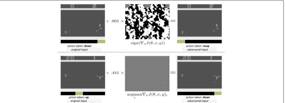
Figure 2 shows the adversarial attack on Pong game
trained with DQN, we can see that after adding small
perturbation to the original clean game background, the trained agent cannot make a correct judgment according to the motion direction of ball. Noting that the adversar-ial examples are calculated by fast gradient sign method (FGSM) (Goodfellow et al.2014a).
FGSM expects the classifier can assign the same class to the real example x and the adversarial examplex˜ with a small enough perturbationηwhich can be concluded as
η=sign(ω) , η∞< (1)
where ω denotes a weight vector, since this
perturba-tion maximizes the change in output for the adversarial examplex˜,ωTx˜=ωTx+ωTη.
Moreover, under image classification network with parameters θ, model input x, targets related to input y, and cost functionJ(θ,x,y). Linearizing the cost function to obtain an optimal max-norm constrained perturbation which can be concluded as
η=sign(∇xJ(θ,x,y)) (2)
In addition, authors also proved that policies trained with reinforcement learning are vulnerable to the adver-sarial attack. However, among the RL algorithms tested in this paper (DQN, TRPO (Schulman et al.2015), and A3C), TRPO and A3C seem to be more resistant to adversarial attack.
Under the domain of Atari game, authors showed that by adding human invisible noises to the original clean game background can make the game unable to work properly, and realize adversarial attack successfully. Huang et al. (2017) gave a new attempt to take adversar-ial research under the scenario of reinforcement learn-ing, and this work proved that the adversarial attack still exists in the domain of reinforcement learning. Moreover, FGSM motivates a series of related research work, Miy-ato et al. (2018) proposed a closely related mechanism to compute the perturbation for a given image, and Kurakin et al. (2016) named this algorithm as “Fast GradientL2” and also proposed a alternative of using ∞for normaliza-tion which named as “Fast GradientL∞”.
Start point-based adversarial attack on Q-learning (SPA) Xiang et al. (2018) focused on the adversarial example-based attack on a representative reinforcement learning named Q-learning in automatic path finding. They pro-posed a probabilistic output model based on the influ-ence factors and the corresponding weights to predict the adversarial examples under such scenario.
Calculating on four factors including the energy point gravitation, the key point gravitation, the path gravitation, and the included angle, a natural linear model is con-structed to fit these factors with the weight parameters computation based on the principal component analy-sis(PCA) (Wold et al.1987).
The main contribution for Xiang et al. is that they built a model, which can generate the corresponding probabilis-tic outputs for certain input points, and the probabilisprobabilis-tic output of our model refers to the possibility of interfer-ence caused by interferinterfer-ence point on the path of agent pathfinding.
Xiang et al. proposed 4 factors to determine wether the perturbation can impact the final result for the agent path planning, which can be concluded as:
Factor Formula expression
Factor 1:
⎧ ⎪ ⎨ ⎪ ⎩
eic=kc+i∗d∗ k
c−kc
√
(kc−kc)2+(kr−kr)2
eir=kr+i∗d∗
1−
kc−kc
√
(kc−kc)2+(kr−kr)2 2
The energy point gravitation
Factor 2: d1i= |aic−kc| + |air−kr|, (kc,kr)=k, (aic,air)=ai∈A The key point
gravitation
Factor 3:
d2i=min{d2|d2= |aic−zjc| + |air
−zjr|,zj∈Z1},(zjc,zjr)=zj,(aic,air)
=ai∈A
The path gravitation
Factor 4: vka=(aic−kc,air−kr),vkt=(tc−kc,tr−kr) cosθi=vka·vkt/|vka||vkt|, θi=arccosθi The included
angle
For Factor 1 can be named as the energy point
grav-itation, which denotes that it is more successful if the adversarial pointkis the point on the key vectorv. Fac-tor 2 is the key point gravitation, which represents that the closer adversarial point is to the key pointk, the more likely it is to cause interference. Factor 3 can be called as the path gravitation, which denotes that the closer adver-sarial point is to the initial pathZ1, the more possible it is to bring about obstruct. Meanwhile, factor 4 can be con-cluded as the included angle, which represents that the angleθ between the vector from the pointkto the adver-sarial point ai and the vector from the key point to the goalt.
Therefore, the probability for each adversarial pointai can be concluded as
pai= 4
j=1
pjai =ω1·aie+ω2·d1i+ω3·d2i+ω4·θi (3)
For this work, the adversarial examples can be found successfully for the first time on Q-learning in path find-ing and their model can make a satisfactory prediction (e.g., Fig.3). Under a guaranteed recall, the precision of the proposed model can reach to 70% with the proper parameter setting. By adding small obstacle points to the original clean map, can interfere the agent’s path finding. However, the experimental map size for this
work is 28 × 28, and there is no additional
verifica-tion for a larger maze map, which can be considered to research in future works. However, Xiang et al. paid attention to the adversarial attack problem in automatic path finding under the scenario of reinforcement learn-ing. Meanwhile this work own practical significance, as the objective for this study is Q-learning which is the most widely used and representative reinforcement learning algorithm.
White-box based adversarial attack on DQN (WBA)
Based on the SPA algorithm introduced above, Bai et al. (2018) proposed that they first use DQN to find the opti-mal path, and analyzed the rules of DQN pathfinding. They proposed a method that can effectively find vulner-able points towards White-Box Q-tvulner-able variation in DQN pathfinding training. Meanwhile, they built a simulation environment as a basic experiment platform to test their method.
Moreover, they classified two types of vulnerable points.
(I) The vulnerable point is most likely on the boundary line. Moreover, the smallerQ(the Q-value difference between the right and downward direction) is the more likely be a vulnerable point is.
For this characteristic of vulnerable pints, they proposed a method to detect adversarial examples. Let P denotes the set of points on the mapP = {P1,P2, ...,Pn}, and each pointPi obtains four Q-values Dij = (Qi1,Qi2,Qi3,Qi4) respectively, which indicate up, down, right, and left. Meanwhile, selecting the direction with the max Q-vale f(Pi) = {j|maxjQij}, and determining wether pointPiis on the boundary line
ϕ(Pi)=OR(f(Pi)!=f(Pi1),f(Pi)!=f(Pi2),
f(Pi)!=f(Pi3),f(Pi)!=f(Pi4)) (4)
wherePij = {Pi1,Pi2,Pi3,Pi4} is the set of the adjoining points for four directions ofPi,A = {a1,a2, ...,an} repre-sents the points on boundary line. Calculating the Q-value differenceQ= |Qi2−Qi3|, and sortingQascending to constructB= {b1,b2, ...,bn}. They took the first 3% of the list as the smallestQ-value points. Finally got the set of suspected adversarial examples, which can be concluded asX= {x1,x−2, ...,xn},X=AB.
For the other type of vulnerable points can be concluded as:
(II) Adversarial examples are related to the gradient of maximum Q-value for each point on the path.
Bai et al. found that when the Q-values of consecutive two points fluctuate greatly, their gradient is greater and they are more vulnerable to be attacked.
Meanwhile, they found that the larger angle between two adjacent lines is, the greater slope of the straight line is. Set angle between the direction vectors of two straight lines to beθ0< θ <π2, the function can be concluded as
cosθ = |s1·s2|
|s1||s2| =
|m1m2+n1n2+p1p2|
m21+n21+p21
m22+n22+p22 (5)
where s1 = (m1,n1,p1),s2 = (m2.n2,p2)are the direc-tion vectors for LineL1,L2. Finally, can find the first large 1% of the angle between the two lines on the path as the suspected interference point.
For WBA, authors successfully found the adversarial examples and the supervised method they proposed is effective, which can be shown in Table2for details. How-ever, in this work, with the increase of training times, the accuracy rate decreases. In other words, when train-ing times are large enough, the interference point can make the path converge, although the training efficiency is reduced.
Similar to the work of Xiang et al., the maps used
for experiment are 16 × 16 and 17 × 17 is size, and
there is no way to verify the proposed adversarial attack method more accurately with such map size. It is rec-ommended that the attack method can be verified on different categories of map-size, which can better illustrate the effectiveness of the proposed method in this paper.
Common dominant adversarial examples generation method (CDG)
Chen at al. (2018b) showed that dominant adversarial examples are effective when targeting A3C path finding,
and designed a Common Dominant Adversarial Examples
Generation Method (CDG)to generate dominant adversarial examples against any given map.
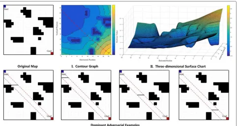
As shown in Fig.4, are the dominant adversarial exam-ples for the original map which can attack successfully.
Chen et al. found that on the dominant adversarial exam-ple perturbation band, the value gradient rises the fastest. Therefore, they call this perturbation band as “gradient band”. By adding obstacles on the cross section of gradi-ent band can perturb the aggradi-ent’s path finding successfully. The generation rule for dominant adversarial example can be defined as:
• Generation Rule:Adding “baffle-like” obstacles to the cross section of gradient band in which the value gradient rises the fastest, can impact A3C path finding.
Moreover, in order to calculate the Gradient Band more accurately, authors considered two kinds of situations according to the difference for original map and gradient function, one situation is that obstacles exist on both sides of the gradient function, and the other is that obstacles exist on one side if the gradient function.
A. Case 1: Obstacles exist on both sides of the gradient function.
As in this case, obstacles exist on the both sides of the gradient curve, then need to
tra-verse all the coordinate points in Obstacle =
{(Ox1,Oy1),(Ox2,Oy2),· · ·,(Oxn,Oyn)}, and to find the
nearest two points from this gradient curve in the upper and lower part respectively. Therefore, the Gradient Band functionFGB(x,y)under such case can be concluded as:
⎧ ⎪ ⎨ ⎪ ⎩
f(x,y)upper=y−(U+a0+a1x+...+akxk)
f(x,y)lower=y−(L+a0+a1x+...+akxk) XL<x<Xmax,YL<y<Ymax
(6)
Table 2Features for adversarial perturbations against single same original clean map, which can show how the different characteristics affect the interference of adversarial example
Number Point coordinates Max Q-value TopQ On the boundary
Point1 (4,5) 90.2229 0.0198 True
Point2 (4,10) 140.7650 0.1616 True
Point3 (2,3) 60.9148 0.2214 True
Point4 (3,4) 71.4446 0.3199 True
Point5 (5,6) 109.0013 0.3595 True
Point6 (0,2) 48.4608 0.4645 True
Point7 (6,7) 126.3412 0.6992 True
Number On the path Top angle size Angle size Perturbation point
Point1 True Ø 74◦ True
Point2 False Ø Ø True
Point3 True Ø 75◦ True
Point4 True 3 69◦ True
Point5 True 1 84◦ True
Point6 True Ø 71◦ True
Fig. 4The first line shows dominant adversarial examples for the original map. The fist picture denotes the original map for attack, and the three columns on the right are the dominant adversarial examples of successful attacks. Meanwhile, the red dotted lines represent the perturbation band. The second line denotes the direction in which the value gradient rises the fastest. By comparison between dominant adversarial examples and the contour graph, can found that on the perturbation band, the value gradient rises fastest
wheref(x,y)upper andf(x,y)lowerdenote the upper/lower bound function respectively,Xmax andYmax denote the boundary value of the map, (XL, 0) and (0,YL) are the intersection points off(x,y)lowerand the coordinate axis.
A. Case 2: Obstacles exist on one side of the gradient function.
In this case, the calculating for distance between obsta-cle edge points and gradient function is same with case 1. However, under such scenario, obstacles exist on one side of the gradient function curve, hence, under this case can only obtain the upper/lower bound function for the Gradi-ent Band. Therefore, the GradiGradi-ent Band functionFGB(x,y) can be concluded as:
⎧ ⎪ ⎪ ⎨ ⎪ ⎪ ⎩
f(x,y)upper=min{f(Xmax, 0),f(0,Ymax)}
f(x,y)lower=y−
L+ a0+a1x+...+akxk
XL<x<Xmax,YL<y<Ymax
(7)
Finally settingY =[ 1, 2, ...,Ymax] andX=[ 1, 2, ...,Xmax] respectively, and generating the obstacle function set Obaffle= {FY1, ...,FX1, ...}
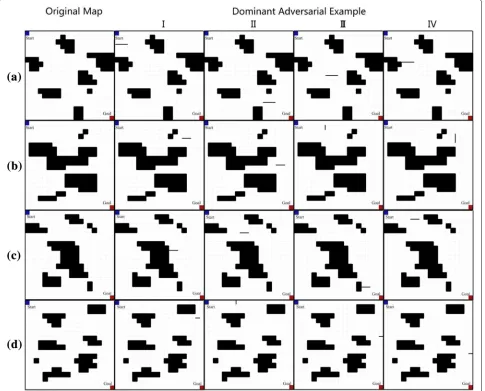
For this paper, the lowest generation precision for CDG algorithm is 91.91% (e.g., Fig.5), which can prove that the method proposed in this work can realize the common
dominant adversarial examples generated under A3C path finding with a high confidence.
This paper showed that, the generation accuracy for adversarial examples of CDG algorithm is relatively high. By adding small obstacles at physical level on the original clean map, it will interfere with the path finding process of A3C agent. Comparing to other works in this field, the experimental map size for Chen’s work contains 10 cate-gories, 10×10, 20×20, 30×30, 40×40, 50×50, 60×60, 70×70, 80×80, 90×90, 100×100, which makes it possi-ble to better verify the effectiveness of the proposed CDG algorithm proposed in this paper.
Black-box attack
Policy induction attack (PIA)
Behzadan and Munir (2017) also discover that Deep Q-network(DQN) based policy is vulnerability under adver-sarial perturbations, and verified that the transferability (Szegedy et al. (2013) proposed in 2013) of adversarial examples across different DQN model does exist.
Fig. 5Samples for Dominant Adversarial Examples. For the first column is the original clean map for path finding. For columns on the right are the samples for Dominant Adversarial Examples generated by CDG algorithm proposed in this paper, and (a), (b), (c), (d) represent four different samples for dominant adversarial examples
network architecture and its parameters at every time step, adversarial examples must be generated by black-box techniques (Papernot et al.2016c).
For every time step, adversary computes the pertur-bation vectors δˆt+1 for the next state st+1 such that maxaQˆ(st+1+ ˆδt+1,a;θt−)causesQˆ to generate its max-imum whena=πadv∗ (st+1). The whole process for policy induction attack can be divided into two parts, namely initialization and exploitation.
The initialization phase must be done before target starts interacting with the environment. Specifically, this phase can be divided as follow:
1) Training DQN policy based on the adversary’s reward functionrto obtain a adversarial strategyπadv∗ . 2) Creating a replica of the target’s DQN and initializing
it with random parameters.
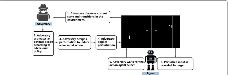
The exploitation phase takes adversarial attack operations (e.g., designing adversarial input), and constitutes the life cycle which can be shown in Fig.6. The cycle is initialized by the first observation value of the environment, and to cooperate with the operation of the target agent.
In the context of policy induction attacks, this paper conjectured that the temporal features of the training pro-cess may be utilize to provide protection mechanisms. However, an analytical treatment of the problem to estab-lish the relationship of model parameters will suggest a deeper insight and guidelines into design a more security deep reinforcement learning architecture.
Specific time-step attack
Fig. 6The exploitation cycle ofpolicy induction attack(Behzadan and Munir2017). For the first phase, adversary will observes the current state, and transitions in the environment. Then adversary will estimate the optimal action to select based on the adversrial policy. For the next phase, adversary take perturbation into application, and perturb the target’s input. Finally, adversary will waits for the action that agent selected
adversarial example at each time step is computed inde-pendently of the adversarial examples at other time step. However, such tactic has not consider the uniqueness of the RL problem.
Lin et al. (2017) proposed two tactics of adversarial attack in the specific scenario of reinforcement learning problem, which namelystrategically-time attack and the enchanting attack.
• Strategically-Timed Attack (STA)
As the reward signal in many RL problems is sparse, an adversary need not attack the RL agent at every time step. Therefore, this adversarial attack tactic utilizes this unique characteristic to attack selected subset of time steps of RL agents. The core of strategically-timed attack is that the adversary can minimize the expected accumulated reward of target agent by strategically attacking less than <<L time steps, to achieve the purpose of adversarial attack, which can be formulated intuitively as an optimization problem
min b1,b2,...,bL,δ1,δ2,...,δL
R1(¯s1, ...,¯sL)
¯
st=st+btδt for all t=1, ...,L bt∈0, 1, for all t=1, ...,L
t
bt≤
(8)
where s1, ...,sL denotes the sequence of observations or states,δ1, ...,δL is the sequence of perturbations,R1 rep-resents the expected return at the first time step,b1, ...,bL denotes when an adversarial example is applied, and the is a constant to limit the total number of attacks.
However, the optimization problem in 8 is a mixed
integer programming problem, which is difficult to solve.
Hence, authors proposed a heuristic algorithm to solve this task, with a relative action preference function c, which computes the preference of the agent in taking the most preferred action over the least preferred action at the current state (similar to Farahmand (2011)).
For policy gradient-based methods such as A3C algo-rithm, Lin et al. defined the functioncas
c(st)=max at π(
st,at)=min at π(
st,at) (9)
wherest denotes the state at time stept, andatdenotes the action at time stept, andπis the policy network which maps the state-action pair(st,at)to a probability.
Meanwhile, for value-based methods such as DQN, the functionccan be defined as
c(st)=max at
eQ(sTt,at)
ake Q(st,ak)
T
−min
at
eQ(sTt,at)
ake Q(st,ak)
T
(10)
whereQdenotes the Q-values of actions, andT denotes the temperature constant.
• Enchanting Attack (EA)
The purpose for enchanting attack is to push the RL agent to achieve the expected statesgafter H steps under the current statest at time step t. Under such attacking approach, the adversary needs to specially design a series of adversarial examplesst+1+δt+1, ...,st+H+δt+H, hence, this tactic of attack is more difficult than strategically-timed attack.
which can make agent to the target satesg from statest. For the second hypothesis, Lin et al. specially designed an adversarial examplest+δtto lure target agent to imple-ment the first action in planned action sequence with
method proposed by Carlini and Wagner (2017). After
agent observes the adversarial examples and takes the first action designed by adversary, the environment will return a new sate st+1 and iterative build adversarial examples in this way. The attack flow forenchanting attack can is shown in Fig.7.
For this work, strategically-time attack can achieve the same effect as the traditional method (Huang et al.2017), while reduce the total time step for attacking. Moreover, enchanting attack can lures target agent to take planned action sequence, which suggests a new research idea for the follow-up studies. Videos are available athttp://yclin. me/adversarial_attack_RL/.
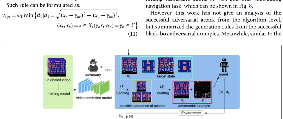
Adversarial attack on VIN (AVI)
The main contribution for Liu et al. (2017) is that they proposed a method for detecting potential attack which can obstruct VIN effectiveness. They built a 2D navigation task demonstrate VIN and studied how to add obstacles to effectively affect VIN’s performance and propose a general method suitable for different kinds of environment.
Their threat model assumed that the entire environ-ment (including obstacles, starting point and destination) is available, and they also know that the robot is trained by VIN, meanwhile, it is easy to get the VIN planning path and the theoretical path. Based on this threat model, they summarized three rules which can effectively obstructing VIN.
• Rule 1: The father away from the VIN planning path, the less disturbance to the path.
Such rule can be formulated as:
v1yk=ω1min
d1|d1=
(xr−ykr)2+(xc−ykc)2, (xr,xc)=x∈X,(ykr,ykc)=yk ∈Y
(11)
wherexr,xcis the coordinate of x,(ykr,ykc)is the coordi-nate ofyk,ω1is the weight ofv1.
• Rule 2: It is most likely to be success when adding obstacles around the turning points on the path.
Such rule can be formulated as:
v2yk=ω2min
d2|d2= max(|tr,−ykr|,|tc−ykc|), (tr,tc)=t∈T,(ykr,ykc)=yk ∈Y
(12)
where(tr,tc)denotes the coordinate of t,(ykr,ykc) repre-sents the coordinate of yk, ω2 is the weight forv2. The formula considers the Chebyshev distance fromyk to the nearest turning point, and utilize the weightω2to control the attenuation ofv2.
• Rule 3: The closer the adding obstacle position is to the destination, the less likely it is to change the path.
The representative for(xnr,xnc)is the coordinate ofxn, (ykr,ykc)denotes the coordinate ofyk,ω3is the weight for v3. Hence, the formula can be concluded as:
v3yk =ω3max(|xnr−ykr|,|xnc−ykc|),(xnr,xnc)
=xn,(ykr,ykc)=yk∈Y (13)
this formula considers the Chebyshev distance fromyk to the destination, and utilize the weightω3 to control the attenuation ofv3.
Calculating the valuevconsidering three rules for each available point, meanwhile, sorting the values to pick up most valuable points S = y|vyk∈maxiV,y∈Y,V = vy1,vy2, ...,vyk.
Liu’s method has great performance on automatically finding vulnerable points of VIN and thus obstructing navigation task, which can be shown in Fig.8.
However, this work has not give an analysis of the successful adversarial attack from the algorithm level, but summarized the generation rules from the successful black-box adversarial examples. Meanwhile, similar to the
Fig. 7Attacking flow forenchanting attack(Lin et al.2017). Enchanting attack from the original statest, the whole processing flow can be concluded
Fig. 8Examples for adversarial examples successfully attack. The examples show that the method proposed in this paper do have ability to find vulnerabilities under VIN pathfinding, and thus interfere the performance of agent automatic pathfinding.aSample of testing set.bAvailable Obstacle 1.cAvailable Obstacle 2.dAvailable Obstacle 3.eAvailable Obstacle 4.fAvailable Obstacle 5
work of Xiang et al. and Bai et al., the map size has too many limitations. Only the size under 28×28 have been experimentally verified, and such size is not enough to prove the accuracy of the method proposed in this paper.
Summary for adversarial attack in reinforcement learning We give summary on the attributions of adversarial attacking methods described above, which can be shown in Table3.
FGSM (Goodfellow et al. 2014a), SPA (Xiang et al.
2018), WBA (Bai et al. 2018), and CDG (Chen et al.
2018b) belong to White-box attack, which have access to the details related to training algorithm and corre-sponding parameters of the target model. Meanwhile,
the PIA (Behzadan and Munir 2017), STA (Lin et al.
2017), EA (Lin et al. 2017), and AVI (Liu et al. 2017) are Black-box attacks, in which adversary has no idea of the details related to training algorithm and corre-sponding parameters of the model, for the threat model discussed in these literatures, authors assumed that the adversary has access to the training environment bat has no idea of the random initializations of the target pol-icy, and additionally does not know what the learning algorithm is.
For White-box attack policies, we summarize the parameters utilized for such methods. SPA, WBA, CDG, PIA, and AVI all have the specific target algorithm,
however, the target for FGSM, STA, anf EA is not single reinforcement learning algorithm, in this sense, such adversarial attack methods are more universal adaptability.
Moreover, the learning way for these adversarial attack methods are different, as FGSM, SPA, WBA, CDG, and AVI are all “One-shot” learning, and PIA, STA, and EA are “Iterative” learning. Additionally, for all attack methods introduced here can generate adversarial exam-ples to achieve the purpose of attacking successfully under a relatively high confidence. The application sce-nario for FGSM, PIA, STA, and EA are Atari game, meanwhile, the scenario for SPA, WBA, CDG, and AVI are all path planning. We also take a statistical anal-ysis of the attack results for the algorithms discussed above.
Modifying input
Adversarial training and its variants • Adversarial training
Adversarial training is the one of the most com-mon strategies in the related literature to improve the robustness of neural networks. By continuously inputting new types of adversarial examples and conducting adver-sarial training, the network’s robustness is continuously improved. In 2015, Goodfellow et al. (2014b) developed a method of generating adversarial examples (FGSM, see (Goodfellow et al. 2014a)), and they also proposed to conduct adversarial training to resist adversarial pertur-bation exploiting the adversarial examples generated by the attack method, the adversarial examples are constantly updated during the training process so that the classifi-cation model can resist the adversarial examples. How-ever, Moosavi-Dezfooli et al. (2017) pointed out that no matter how many adversarial examples are added, there are new adversarial examples that can cheat the trained networks in 2017. After that, by combining adversarial examples with other methods, researchers have produced better approaches defending adversarial examples in some recent works.
• Ensemble adversarial training
It trains networks by utilizing the several pre-trained vanilla networks to generate one-step adversarial exam-ples. The model by adversarial training can defend weak perturbations attack but can’t defend against strong ones. Based on this, Florian Tramer et al. (2017) introduced the ensemble adversarial training, which enhances training data with perturbations transferred from other static pre-trained models, this approach separates the generation of adversarial examples from the model being trained, simul-taneously drawing an explicit connection with robustness to black-box adversaries. This model trained by ensem-ble adversarial training has strong robustness to black-box attacks on ImageNet.
• Cascade adversarial training
For unknown iterative attacks, Na et al. (2018) proposed cascade adversarial training, they trained the network by inputting adversarial images generated from the iterative defended network and one-step adversarial images from the network being trained. At the same time, the authors regularized the training with a unified embedding so that the convolution filters can gradually learn how to ignore pixel-level perturbations. The cascade adversarial training is shown in Fig.9.
• Principled adversarial training
From the perspective of distributed robust optimiza-tion, Aman Sinha et al. (2018) provided a principled
adversarial training, which guaranteed the performance of neural networks under adversarial data perturbation. By utilizing the Lagrange penalty form of perturbation under the potential data distribution in the Wasserstein ball, the authors provide a training process that uses worst-case perturbations of training data to reinforce model parameter updates.
• Gradient Band-based Adversarial Training
Chen et al. (2018b) proposed a generalized attack
immune model based on gradient band, which can be shown in Fig.10, mainly consists ofGeneration Module, Validation Module, andAdversarial Training Module.
For the original clean map, Generation Module can
generate dominant adversarial examples based on the Common Dominant Adversarial Examples Generation Method (CDG) (see Section 3.2.4). Validation Module can utilize the well trained A3C agent against the origi-nal clean map, to calculate the Fattack for each example based on the success criteria for attack proposed in this paper.Adversarial Training Moduleutilize a single exam-ple which can attack successfully for adversarial training, and obtain a newly well trained A3Cagentnew which can finally realize “1:N” attack immunity.
Data randomization
In 2017, Xie et al. (2017) found that introducing random resizing to the training images can reduce the strength of the attack. After that, they further proposed (Xie et al. 2018) to use randomization at inference time to mitigate the effects of adversarial attack. They add a random resize layer and a random padding layer before the network of classification, their experiments demonstrate that the pro-posed randomization method is very effective at resisting one-step and iterative attacks.
Input transformations
Guo et al. (2018) proposed strategies to defend against adversarial examples through transforming the inputs before feeding them to the image-classification sys-tem. The input transformations include bit-depth reduc-tion, JPEG compression, total variance minimizareduc-tion, and image quilting before feeding the image. And the authors showed that total variance minimization and image quilt-ing are very effective defenses on ImageNet.
Input gradient regularization
Fig. 9The structure of cascade adversarial training
regularization with adversarial training, but the computa-tional complexity is too high.
Modifying the objective function Adding stability term
Zheng et al. (2016) conducted stability training through adding stability term to the objective function to encourage DNN to generate similar output for images of various per-turbed versions. The perper-turbed copyIof the input image I is generated by a Gaussian noise , the final loss Lis consisted of the task objective Lo and the stability loss Lstability.
Adding regularization term
Yan et al. (2018) append the regularization term based on adversarial perturbations to the objective function, they proposed a training recipe called “deep defense”.
Specifically, the authors optimize the objective function jointed the original objective function term and a scaled
xp as a regularization term. Given a training set
{(xk,yk)}and the parameterized functionf, andWcollects learnable parameters off, the new objective function can be optimized as bellow:
min W
k
L(yk,f(xk;W))+λ k
R
−xkp
xkp
(14)
By combining an adversarial perturbation-based regular-ization with the classification objective function, the train-ing model can learn to defend against adversarial attacks directly and accurately.
Dynamic quantized activation function
Rakin et al. (2018) first explored to use quantization of activation functions and proposed to exploit adaptive
quantization techniques for the activation functions so that training the network to defend against adversarial examples. They show the proposed Dynamic Quantized Activation(DQA) method greatly heightened the robust-ness of DNN under white-box attack, such as FGSM (Goodfellow et al.2014a), PGD (Madry et al.2017), and C&W (Carlini and Wagner2017) attacks on MNIST and CIFAR-10 datasets. In this approach, the authors integrate the quantized activation functions into on adversarial training method, in which training model to learn param-etersγ to minimize the riskR(x,y)∼L[J(γ,x,y)],γ consists of parameters in DNN. Based on this, given the input image xand the adversary examplex+, this work aim to min-imize the objective function to enhance the robustness
minR(x,y)∼L[maxJ([γ,T],x+,y)] (15)
where adding a new set of learnable parameters T :=
[t1,t2, ...,tm−1]. For n-bit quantized activation function, the quantization will have 2n−1 threshold valuesT, let m=2n−1,sgnrepresents the sign function, thenmlevel quantization function is as follows:
f(x)=0.5× ⎡
⎣sgn(x−tm−1)+ m/2+1
i=m−1
ti(sgn(ti−x)
+sgn(x−ti−1))+
2
i=m/2
ti−1(sgn(ti−x)
+sgn(x−ti−1))−sgn(t1−x)
⎤ ⎦
(16)
Stochastic activation pruning
Inspired by game theory, S. Dhillon et al. (2018) proposed a mixed strategy Stochastic Activation Pruning (SAP) for adversarial defense. The method prunes a random acti-vation subset (preferentially pruning those with smaller magnitude) and expands survivors to compensate, using SAP to pretrained networks without any additional train-ing provides robustness against adversarial examples. And the authors showed that combining SAP with adversar-ial examples has a greater benefits. In particularly, their experiments demonstrate that SAP can effectively defend against adversarial examples in reinforcementlearning.
Modifying the network structure Defensive distillation
Papernot et al. (2016a) proposed the defensive distilla-tion mechanism for training network to resist adversarial attacks. Defensive distillation, a strategy that trains mod-els to output the probability of different classes rather than the difficult decision of which class to output, the prob-ability is provided by an early model that uses the labels of hard classification to train on the same task. Papernot
et al. showed that defensive distillation can be used to resist small-disturbed adversarial attacks through training network to defend L-BFGS (Szegedy et al.2013) attack and FGSM (Goodfellow et al. 2014a) attack. Unfortunately, defensive distillation is only applicable to DNN models based on energy probability distributions. Nicholas Car-lini and David Wagner proved that defensive distillation is ineffective in (Carlini and Wagner 2016), and they introduced a method of constructing adversarial examples (Carlini and Wagner2017), this method is not affected by various anti-attack methods, including defensive distillation.
High-level representation guided denoiser
Liao et al. (2018) proposed high-level representation guided denoiser (HGD) to defend adversarial exam-ples for image classification. The main idea is to train a denoiser based on neural network for remov-ing the adversarial perturbation before sendremov-ing them to the target model. FLiao et al. use denoising U-net
(Ronneberger et al. 2015) (DUNET) as a
denois-ing model. Compared to denoisdenois-ing autoencoder (DAE)
(Vincent et al. 2008), DUNET is directly connected
between encoder layers and decoder layers of the same resolution, so the network only needs to learn how to remove noise, instead of learning how to reconstruct the whole image. And without using a pixel-level reconstruc-tion loss funcreconstruc-tion, the authors use the difference between top-level outputs of the target model induced by orig-inal and adversarial examples as the loss function to guide the training of an image denoiser. The proposed HGD has a good generalization and the target model is more robust against both white-box and black-box attacks.
Add detector subnetwork
Metzen et al. (2017) proposed to add a detector network for augmenting deep neural networks, the sub-network is trained on a binary classification task that distinguishes real data from data containing adversarial perturbations. Considering that detector is also adver-sarial, they proposed dynamic adversary training, which introduces a novel adversary that aims at fooling both the classifier and the detector, and trains the detector to coun-teracting this novel adversary. The experiment results show that dynamic detector has the robustness and its detectability is more than 70% on the CIFAR10 dataset (Krizhevsky and Hinton2009).
Multi-model-based defense
Srisakaokul et al. (2018) explored a novel defense
each other to obtain robustness diversity, specifically, the adversarial examples of a model usually doesn’t be the adversarial examples of other models in model family. Then the method randomly selects one model in these models to be applied on a given input example. The ran-domness of selection reduces can reduce the success rate of the attack. The evaluation results demonstrate that MULDEF augmented the adversarial accuracy of the tar-get model by about 35-50% and 2-10% in the white-box and black-box attack scenarios, respectively.
Generative models • PixelDefend
Song et al. (2017) proposed a method named
Pix-elDefendwhich can utilized generative models to defend against adversarial examples. In this paper, authors showed that the adversarial examples mainly lie on low probability regions of training distribution, regardless of the attack type and target model. Moreover, they found that neural density model outperform on detecting the human invisible adversarial perturbations, and based on this discovery, Song et al. proposed a new approach namedPixelDefendwhich can purifies a perturbed image return to the distribution of training data. Meanwhile,
they announced that PixelDefend can be utilized as
a novel family of methods which can combined with other model-specific defenses. Experimental results (e.g., Fig. 11) showed that PixelDefend can greatly improves the recovery capability of varieties state-of-art defense methods.
• Defense-GAN
Samangouei et al. (2018) gave the first attempt to con-struct a defense model against adversarial attack based on GAN (Radford et al.2015). They proposed a new defense policy namedDefense-GANwhich takes use of generation
model to improve the robustness against
Black/White-Box Attack. Moreover, any classification model can
uti-lize the Defense-GAN proposed in this paper, and will
not change the structure of classifier or the process for
training. Defense-GAN can be used as a defense
tech-nology that can against any adversarial attack as such method does not assume knowledge of the process for generating the adversarial examples. The experimental results showed thatDefense-GAN proposed in this paper is effective when against different adversarial attacks, and can improve the performance on existing defense tech-nologies.
Discriminative model
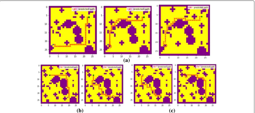
Since it is not guaranteed that the generated adversarial examples will obstruct the VIN path planning success-fully generated in Liu et al. (2017), Wang et al. explored a fast approach to automatically identify VIN adversar-ial examples. In order to estimate whether an attack is successful, they compared the difference between the two paths on a pair of maps, the normal map and the adver-sarial map. By visualizing the pair of paths on a path image, they transformed the different attack results into different categories of path images. In this way, they ana-lyzed the possible scenarios of the adversarial maps and define the categories of the predicted path pairs. They divided the results into four limited categories, which are the unreached path (UrP) class, the fork path (FP) class, the detour path (DP) class and the unchanged path (UcP) class. Based on the categories definition, they implemented a training-based identification method by combining the path feature comparison and path images classification.
In this method, the UrP and UcP can be identified through path feature comparison and the DP and FP can be identified through path image classification. The experimental results showed that this method can achieve
(a)
(b)
(c)
(d)
Fig. 12Four categories of VIN adversarial maps. The first line denotes the original maps, the second line represents the adversarial eaxmples generated, and the third line is the extracted path image.aThe UrP.bThe FP.cThe DP.dThe UcP
Table 4Different attacks targeted by different defense technologies
Modifying input FGSM IFGSM PGM CDG DeepFool C&W JSMA ITGSM
Adversarial training
Ensemble adversarial training
Cascade adversarial training
Principled adversarial training
Gradient band-based adversarial training
Data randomization
Input transformations
Input gradient regularization
Modifying the objective function FGSM DeepFool C&W Small perturbations PGD
Adding stability term
Adding regularization term
Dynamic quantized activation function
Stochastic activation pruning
Modifying the network structure FGSM IFGSM DeepFool C&W JSMA ITGSM BIM Opt
Defensive distillation
High-level representation Guided Denoiser
Add detector subnetwork
Multi-model-based defense
Generative models
a high-accuracy and faster identification than manual observation method (e.g., Fig.12).
Characterizing adversarial subspaces
Ma et al. (2018) gived the first attempt to explain the extent adversarial perturbation can effect theLocal Intrin-sic Dimensionality (LID) (Houle 2017) characteristic of adversarial regions. Moreover, they showed empirically that LID characteristics can facilitate the distinction of adversarial examples generated by several state-of-art attacks. Meanwhile, they proved that LID can be utilized to differentiate adversarial examples, and the experimen-tal results show that among the five attack strategies
(FGSM (Goodfellow et al. 2014a), BIM-a (Saad 2003),
BIM-b (Saad 2003), JSMA (Papernot et al.2016b), Opt) based on three benchmark data sets (MNIST (LeCun et al. 2010), CIFAR-10 (Krizhevsky et al.2014), SVHN (Netzer et al.2011)) considered for this paper, the method based on LID can outperform against most state-of-art methods. Ma et al. announced that their analysis of LID charac-teristic for adversarial region, not only can motivates new direction for effective adversarial defense, but also pro-vides more challenges for the development of new adver-sarial attacks, meanwhile, enable us to better understand the vulnerabilities of DNNs (LeCun et al.1989).
Conclusion and discussion
In this paper, we give the very first attempt to con-duct a comprehensive survey on adversarial attacks in the context of reinforcement learning under AI security. Reinforcement learning is a workhorse for AI applications
ranging fromAtari Game to Connected and Automated
Vehicle System(CAV), hence, how to build a reliable rein-forcement learning system to support the security critical applications in AI, has become a concern which is more critical than ever. However, Huang et al. (2017) discovered that the interesting attack modeadversarial attackalso be effective when targeting neural networks under reinforce-ment learning, which has inspired innovative researches in this direction. Therefore, our work reviews such con-tributions, and mainly focus on the most influential and interesting works in this field. We give a comprehensive introduction to the literatures on adversarial attack under various fields of reinforcement learning applications, and briefly analyze the most valuable defense technologies against existing adversarial attacks (Table4).
Although, the RL system does exist the security vulner-ability of “Adversarial attack”, by the survey on existing adversarial attack technologies, it is found that the exist of complete Black-box attacks are rare (complete Black-box attack means that the adversary has no idea of the tar-get model, and can not interact with the tartar-get agent at all), which makes it very difficult for adversaries to attack the reinforcement learning system in practice. Moreover,
owing to the very high activity in this research direction, it can be expected that, in the future an largely reliable reinforcement learning system will be available to support critical security applications in AI.
Acknowledgements
The authors would like to thank the guidance of Professor Wenjia Niu and Professor Jiqiang Liu. Meanwhile this research is supported by the National Natural Science Foundation of China (No. 61672092), Science and Technology on Information Assurance Laboratory (No. 614200103011711), the Project (No. BMK2017B02-2), Beijing Excellent Talent Training Project, the Fundamental Research Funds for the Central Universities (No. 2017RC016), the Foundation of China Scholarship Council, the Fundamental Research Funds for the Central Universities of China under Grants 2018JBZ103.
Funding
This research is supported by the National Natural Science Foundation of China (No. 61672092), Science and Technology on Information Assurance Laboratory (No. 614200103011711), the Project (No. BMK2017B02-2), Beijing Excellent Talent Training Project, the Fundamental Research Funds for the Central Universities (No. 2017RC016), the Foundation of China Scholarship Council, the Fundamental Research Funds for the Central Universities of China under Grants 2018JBZ103.
Availability of data and materials Not applicable.
Authors’ contributions
TC conceived and designed the study. TC and YX wrote the paper. JL, WN, ET, and ZH reviewed and edited the manuscript. All authors read and approved the manuscript.
Authors’ information
Wenjia Niu obtained his Bachelor degree from Beijing Jiaotong University in 2005, PhD degree from Chinese Academy of Science in 2010, all in Computer Science. Now he is currently a professor in Beijing Jiaotong University. His research interests are AI Security, Agent and Data Mining. He has published more than 50 research papers, including a number of regular papers in the famous international journals and Conferences, such as KAIS (Elsevier), ICDM, CIKM and ICSOC. He has published 2 edited books. He serves on the Steering Committee of ATIS (2013-2016) and the PC Chair of ASONAM C3’2015. He has been PhD Thesis Examiner of Deakin University, Title Page Click here to access/download;Title Page;cover letter.pdf the guest editor for the Chinese Journal of Computer, Enterprise Information System, Concurrency and Computing: Practise and Experience, and Future Generation Computer Systems, etc.. He is also members both of the IEEE and ACM.
Competing interests
The authors declare that they have no competing interests.
Publisher’s Note
Springer Nature remains neutral with regard to jurisdictional claims in published maps and institutional affiliations.
Received: 31 October 2018 Accepted: 12 February 2019
References
Akhtar N, Mian A (2018) Threat of adversarial attacks on deep learning in computer vision: A survey. arXiv preprint arXiv:1801.00553 Bai X, Niu W, Liu J, Gao X, Xiang Y, Liu J (2018) Adversarial Examples
Construction Towards White-Box Q Table Variation in DQN Pathfinding Training. In: 2018 IEEE Third International Conference on Data Science in Cyberspace (DSC). IEEE. pp 781–787
Behzadan V, Munir A (2017) Vulnerability of deep reinforcement learning to policy induction attacks. In: International Conference on Machine Learning and Data Mining in Pattern Recognition. Springer, Cham. pp 262–275 Bougiouklis A, Korkofigkas A, Stamou G (2018) Improving Fuel Economy with