Hydrologic Calculator: An Educational Interface for Hydrological Processes Analysis

Hydrologic Calculator: an educational interface for hydrological

processes analysis

Narendra Singh Raghuwanshi

_{, Rajendra Singh}

_{, Sirisha Adamala}

_,

Akhilesh Prasad

_{, Ashish Chamoli}

(1. Professor, Agricultural and Food Engineering Department, IIT Kharagpur, Kharagpur-721302, West Bengal, India; 2. Scientist, Natural Resources Management Division, Central Island Agricultural Research Institute (CIARI), Port Blair-744101,

Andaman and Nicobar Islands, India;

3. Sr R&D Engineer, Synopsys Inc, Mountain View, California-94043, USA; 4. Technical Team Leader, IBM India Pvt. Ltd., Pune-411006, Maharashtra, India)

Abstract: Hydrology, which deals with the study of water, is one of the fundamental courses to the undergraduate program of

many disciplines: civil engineering, agricultural engineering, earth sciences, environmental sciences, geography, etc. This course covers various events of the hydrological cycle, namely, rainfall, runoff, hydrograph, infiltration, evapotranspiration, and flood routing. These events involve a large number of techniques and methods for the analysis, which are time-consuming. To enhance the learning, this study presents a tool called ‘Hydrologic Calculator’, an educational interface with eight modules for analyzing the various hydrological related events. In addition, ‘Help’ module in ‘Hydrologic Calculator’ provides a thorough understanding of the theory and methodology adopted for solving the different hydrological problems. Hydrologic Calculator includes a graphical user interface, which helps in input data preparation and output display in both graphical and tabular forms. Besides, it also provides detailed results in log (.txt) format. All the eight modules of the software were tested using the available published data. The validation results obtained using Hydrologic Calculator were in good agreement with the respective results given in the source. Thus, Hydrologic Calculator can be used as a professional computer tool for teaching and analyzing different hydrological processes.

Keywords: Hydrologic Calculator, Visual Basic 6, hydrograph, runoff, rainfall, infiltration, evapotranspiration

Citation: Raghuwanshi, N. S., R. Singh, S. Adamala, A. Prasad, and A. Chamoli. 2019. Hydrologic Calculator: an educational

interface for hydrological processes analysis. Agricultural Engineering International: CIGR Journal, 21(1): 1– 17.

1 Introduction

The hydrologic cycle deals with many processes, e.g., rainfall, condensation, evaporation, transpiration, and runoff. All these processes play a vital role in the protection and management of not only water resources but also several environmental resources. As a result, hydrology these day forms a part of educational curricula of diverse engineering and science disciplines: agricultural, civil, environmental, geography, geology,

Received date: 2017-11-24 Accepted date: 2018-01-19

* Corresponding author: Sirisha Adamala, Scientist, Natural

Resources Management Division, Central Island Agricultural Research Institute (CIARI), Port Blair-744101, Andaman and Nicobar Islands, India. Email: [email protected], Tel: 09948484983.

al., 2007, 2012). Therefore, a specific type of education with the introduction of computer simulation modules is needed during under graduation level such that they cover not only the basic hydrological concepts but also to deal with the real world problems. These computerized techniques afford instructors the opportunity to have their students engage in realistic and authentic problem based on activities without the need to manage other logistical constraints often encountered with field research (i.e., transportation, materials, etc.).

As such, the hydrologic research community has expressed the need for fundamental improvements in current practices of hydrologic education, especially at the undergraduate level (Bourget, 2006; Wagener et al., 2007; Howe, 2008; Loucks, 2008; Ledley et al., 2008; CUAHSI, 2010;Ngambeki et al., 2012; Pathirana et al., 2012; Uhlenbrook and de Jong 2012). In recent years, a series of publications has recognized and reviewed the challenges in emphasizing the introduction of new computer based on pedagogies in hydrology education.

Sanchez et al. (2015) demonstrated that the computerized learning in hydrology context can effectively bring the “real world” into the classroom and make it accessible, especially in the case of undergraduate students. Merwade and Rudell (2012) stated that traditional classroom with lecture-format pedagogy plays a critical role in delivering hydrology concepts to students, but there is a need to explore how these traditional approaches can be augmented with new pedagogies that include the use of digital data, simulation and visualization tools to enhance students’ learning. Ruddell and Wagener (2015) reviewed how hydrology education has evolved over the decades, where the community (especially United States and European) appears to be headed, and ‰rand challenges in the 21st

century. The challenges include development of formal pedagogies, new technologies, and a broadening and globalization of hydrology education. Habib et al. (2012) designed and evaluated a web-based educational tool called ‘HydroViz’ to support active learning in hydrology education. This tool basically simulates the real-world natural hydrologic systems by learning model either with filed data or with stored random computer data.

The findings of the above papers strengthen the fact

that it is possible to introduce or improve the undergraduate hydrological curriculum with a small effort in the way of computer modeling and programming. Further, hydrological processes analysis is time consuming and often requires the standard text to perform the analysis. Therefore, there is a need to develop a tool for performing hydrological processes analysis. In the past, a number of graphical user interface (GUI) based computer software has been developed for analyzing the different hydrological variables. Some of the early developed software in the field of hydrology include: RRL (Perraud et al., 2003) for rainfall-runoff analysis; WHAT (Lim et al., 2005), WBNM (Boyd et al., 1996), and IHACRES (Allen and Liu, 2011) for hydrograph analysis; RAINBOW (Raes et al., 2006) for hydro-meteorological frequency analysis; HEC-SSP (Harris et al., 2010) for rating curve analysis; SIDES (Adamala et al., 2014a) for surface irrigation design; and DSS_ET (Bandyopadhyay et al., 2012) for evapotranspiration estimation.

All the above software have been developed only to analyze any one of the various hydrological processes. These softwares do not have a single platform based comprehensive module for all hydrological processes/events. Further, these softwares are good for research and design but lack in the stepwise design process, which is essential for undergraduate student learning. Therefore, the present study is carried out an aim to develop a user-friendly software package for analyzing and solving different hydrologic processes and yield a step-wide design procedures for thorough understanding. Use of this software is encouraged to reduce the time required to reach a solution.

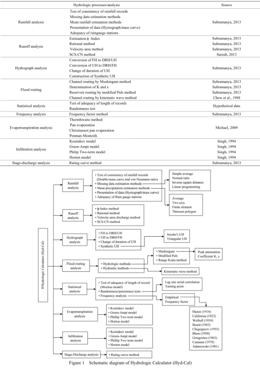
2 Theoretical background

Table 1 Analysis of various hydrological processes

Hydrologic processes/analysis Source

Test of consistency of rainfall records Missing data estimation methods Mean rainfall estimation methods

Presentation of data (Hyetograph/mass curve) Rainfall analysis

Adequacy of raingauge stations

Subramanya, 2013

Estimation φ -Index Subramanya, 2013

Rational method Subramanya, 2013

Velocity-area method Subramanya, 2013

Runoff analysis

SCS-CN method Suresh, 2013

Conversion of FH to DRH/UH Conversion of UH to DRH/FH Change of duration of UH Hydrograph analysis

Construction of Synthetic UH

Subramanya, 2013

Channel routing by Muskingum method Subramanya, 2013

Determination of K and x Subramanya, 2013

Reservoir routing by modified Puls method Subramanya, 2013 Flood routing

Channel routing by kinematic wave method Chow et al., 1988 Test of adequacy of length of records

Statistical analysis

Randomness test Hypothetical data

Frequency analysis Frequency factor method Subramanya, 2013

Thornthwaite method Pan evaporation

Christiansen pan evaporation Evapotranspiration analysis

Penman-Monteith

Michael, 2009

Kostiakov model Singh, 1994

Green-Ampt model Singh, 1994

Philip Two-term model Singh, 1994

Infiltration analysis

Horton model Singh, 1994

Stage-discharge analysis Rating curve method Subramanya, 2013

2.1 Rainfall analysis

Rainfall analysis includes test of consistency of rainfall records (double mass curve, Von Neuman Ratio method), missing data estimation (simple average, normal ratio, inverse square distance and linear programming method), mean areal rainfall estimation (simple average, two-axis, finite element, and Theissen polygon method), representation of rainfall using hyetograph and mass curve, and raingauge networks analysis (Table 1).

2.1.1 Von Neuman Ratio (VNR) test for consistency of rainfall records

Many hydrological studies require long-term rainfall data; therefore, a test must be conducted to check self-consistency of the rainfall records. The consistency of rainfall records can be checked using VNR test. The VNR test is basically based on statistics and is also called as a ‘statistical test’. Let Pi (i=12,3,…,n), denotes the

departures from some average of rainfall value, whose consistency is to be tested. The test can be expressed as:

1 2 1 1 2 1 ( ) ( ) n i i i n i i P P V P P + + = = − = −

∑

∑

where, P and P= rainfall and mean rainfall values; n = number of data points in rainfall series. For a non-homogeneous record, the value of V should be less than 2 or vice-versa.

2.1.2 Estimation of missing rainfall data

The point observation from a rainfall gauge may have a short break in the records due to instrument failure or absence of the observer. Therefore, it is often necessary to estimate the missing records using data from the neighboring stations. The inverse square distance (ISD) method is the most suitable method to estimate the missing rainfall data (Px) at station ‘x’, which connects it to nearest raingauge (of known rainfall data) stations and measures the distances x1, x2, x3,..., xn. Therefore, the

weight of each station (Wi = 1/xi2) with respect to station

‘x’ can be used to calculate the missing rainfall (Px) as

follows: 1 1 n i i i x n i i PW P W = = =

∑

∑

Unlike the other methods, the linear programming (LP) method does not determine the weighting factors beforehand (Singh, 1994). It selects the base station and several surrounding index stations and determines optimal weighting factors, by minimizing the deviations between observed and computed rainfall at a base station for a number of rainfall events.

Suppose the weight assigned to the each index stations is W1, W2, W3, …Wn and rainfall is P1j, P2j, P3j, …Pnj and rainfall at the base station is Pbj for jthevent.

The deviation is a difference between the computed

( 1 n i ij i W P =

∑

unrestricted in sign if both the quantities are positive. Hence, it is replaced by the difference of two positive quantities (uj, vj). Therefore, the objective is to minimize

the sum of these two positive quantities as follows:

Minimization: 1 ( ) k j j j

Z u v

=

=

∑

(3) Subjected to the constraints:

1

n

i ij j j bj

i

W P u v P

=

− + =

∑

0 i

W ≥ for i = 1, 2, 3, ……, k (5)

0, 0

j j

u ≥ v ≥ for j = 1, 2, 3, …., k (6)

After finding weight at each station, the value of rainfall at missing raingauge station can be found as follows:

1

n

b i i

i

P W P

=

=

∑

2.1.3 Conversion of point rainfall to areal rainfall Mean areal rainfall is required for many engineering applications, which can be estimated from the group of point rainfall events in a watershed of n number of raingauge stations. It is most commonly estimated using the simple average, Theissen polygon, and Isohyetal methods. The alternative methods are Two-Axis (Bethlahmy, 1976) and Finite Element (Akin, 1971) methods.

2.1.3.1 Two-Axis method

bisector (minor axis). Further, draw two lines from each of the gages, one line to farther end of the major axis, the other to the farther end of the minor axis. Define the coordinates of the gauging stations in terms of x and y

coordinates, i.e. for an ith gauge, the coordinates are (x, y) and the rainfall measured is donated by Pi. The acute

angle between these two lines θ is measured and subsequently the areal rainfall over a given area can be determined as follows:

1

1

n

i i i

n

i i

θP P

θ

= =

=

∑

∑

Connect the number of gauging stations in a watershed arbitrarily to form m triangular sub-areas. Assign an identification number to each gauging station, beginning with one. Assume the rainfall over the sub-area varies linearly between the three gauging points. Therefore, for an ith gauge interior to the nth sub-area, the rainfall can be expressed as:

1 2 3

( , )

ni n n i n i

p x y =a +a x +a y (9)

1 2 3

( , )

nj n n j n j

p x y =a +a x +a y (10)

1 2 3

( , )

nk n n k n k

p x y =a +a x +a y (11)

where, ani= constant related to the rainfall measurements

at the corners. The above equation is also valid for the corners of the sub-areas.

Solve the above simultaneous equations for an1, an2

and an3, and calculate volume of rainfall at any point

within the subarea (Vn) as:

1 2 3

1 1

( ) ( )

3 3

n n n n i j k n i j k

V =A a_⎢⎡ +a x +x +x +a y +y +y ⎤_⎥

⎣ ⎦(12)

where, An = area of sub triangle.

Compute the total volume (V) and area (A) of rainfall over the triangular mesh as:

1

m

i i

V V

=

=

∑

1

m

i i

A A

=

=

∑

Compute the mean areal rainfall (P) as:

V P

A

= (15)

2.2 Flood routing

Flood routing deals with determination of time and magnitude of a flood wave at a section of a river (i. e. Flood hydrograph at the section) by utilizing the data of flow at one or more upstream section. There are several methods available for flood routing and they can be further classified into two groups:

i. Hydrologic routing: methods under this category employ equation of continuity.

ii. Hydraulic routing: methods under this category employ equation of continuity and equation of motion for unsteady flow.

Hydrologic routing can be further classified into reservoir routing and channel routing. In Hydrology calculator, the Modified Puls method is used for reservoir routing and Muskingum routing method and Runge-Kutta method are used for channel routing. Under hydraulic routing category, kinematic wave method of channel routing is used and is briefly described below.

2.2.1 Kinematic wave method (channel routing)

The kinematic wave model consists of continuity equation and a simplified form of the momentum equation, based on the assumption that the energy grade line is parallel to the channel bottom slope, i.e., the acceleration and pressure terms in the momentum equation are negligible. The kinematic wave model is defined by the following equations:

Continuity equation, Q A q

x t

∂ ₊∂ ₌

∂ ∂ (16)

Momentum equation, So=Sf (or)

3/5 2/3

3/5

1.49 _o

nP

A Q

S

⎛ ⎞

= ⎜_⎜ ⎟_⎟

⎝ ⎠

(17) Equations (16) and (17) can be combined for kinematic wave approximation with only Q as dependent variable as follows:

Equation of continuity becomes, Q _αβQβ 1 Q _q

x t

−

∂ ₊ ⎛∂ ⎞₌

⎜ ⎟

∂ ⎝ ∂ ⎠

(18) where, Q = flow along the length (x) of channel; So =

channel bed slope; Sf =slope of the energy line; n =

manning’s roughness coefficient; q = lateral inflow into the channel; y = depth of flow; B = width of the channel;

perimeter (B+2y, for B>>y); α and β = parameters. Equation (18) is solved by the backward-difference (finite difference) method to determine the outflow hydrograph from inflow hydrograph for given value of channel parameters α and β, the lateral inflow q(t) and initial and boundary conditions. The finite difference form of the space derivative is found by substituting the value of Q on the (j+1)th time as:

1 1 1 Δ j j i i Q Q Q x x + + + − ∂ ₌

∂ (19)

where, Δx = length along the channel between two segments; i and j denotes the distance along the channel length and time, respectively.

The finite difference form of the time derivative is found likewise by substituting the value of Q on the (i+1)th _{distance as:}

1 1 1 Δ j j i i Q Q Q t t + + − + ∂ ₌

∂ (20)

where, Δt = time interval.

If the value of Q were used in ‘αβQβ-1_{’ term,}

1 1 2 j j i i Q Q Q + + +

= (21)

The value of lateral inflow q is found by averaging the value of the (i+1)th _{distance (these are assumed to be}

given in the problem)

1 1 1 2 j j i i q q q + + + +

= (22)

By substituting Equations (19) to (22), Equation (18) becomes:

1

1 1 1 1

1 1 1 1

1

1 1

2

2

β

j j j j j j

i i i i i i

j j

i i

Q Q Q Q Q Q

αβ

Δx Δt

q q − + + + + + + + + + + + ⎛ ⎞ ⎛ ⎞ − ₊ + − ⎜ ⎟ ⎜ ⎟ ⎝ ⎠ ⎝ ⎠ + = (23)

This equation is solved for the unknown 1 1

j i

Q +

+ as

follows:

1 1

1

1 1

1 1 1 1

1 1 1 1 Δ Δ

Δ 2 2

Δ

Δ 2

j i

β

j j j j

j j i i i i

i i

β

j j

i i

Q

Q Q q q

t

Q αβQ t

x Q Q t αβ x + + − + + + + + + + − + + = ⎡ _{⎛ + ⎞ ⎛ + ⎞}⎤ ⎢ + _{⎜ ⎟} + _{⎜ ⎟}⎥ ⎢ ⎝ ⎠ ⎝ ⎠⎥ ⎣ ⎦ ⎡ _{⎛ + ⎞} ⎤ ⎢ + _{⎜ ⎟} ⎥ ⎢ ⎝ ⎠ ⎥ ⎣ ⎦ (24)

By using above equation 1 1

j i

Q +

+ can be found out for

given value of Δt, Δx, α, β, j₁ i

q₊ , 1

1

j i

q +

+ , 1

j i

Q₊ , j 1

i

Q + _.

2.3 Frequency analysis

Frequency analysis deals with the chance of occurrence of an event over a specified period of time. Suppose, P is the probability of occurrence of an event (rainfall) whose magnitude is equal to or in excess of a specified magnitude X. The recurrence interval (return period) is related to P as follows:

1

T P

= (25)

Before performing frequency analysis data should be checked for adequacy of the length of the record and randomness.

2.3.1 Test of adequacy of length of record

To check the adequacy of the length of record, Mockus (1960) developed the following equation:

2 min (4.3 log10 2) 6

Y = t Q + (26)

where, Ymin = minimum acceptable years of record; t10 =

Student “t” value at 10% significance level, and Q2 = ratio

of 100 year maximum rainfall to two year maximum rainfall and is defined as below:

100 2 2 T T Z Q Z = =

= (27)

(1 )

T V T

Z =Z +C C (28)

where, ZT = annual rainfall for T years recurrence interval;

Z= mean annual rainfall of the sample; CV = coefficient

of variation of the sample; and CT = frequency factor, and

is determined as follows:

(

)

{

}

2.45

0.577 ln ln ln 1

3.1416 T

C = − ⎡_⎣ + T − T− ⎤_⎦ (29)

2.3.2 Test for randomness or persistence test

Hydrologic data must be checked for independence. The independence means that the outcome of the hydrologic variable (rainfall amount) at a given time does not depend on the value of the variable at a previous time. The Lag one serial correlation and Turning point tests can be used for checking the independence of the hydrologic data.

(

)(

)

(

)

X X X X

N r X X N − + = = − − − = −

∑

∑

where, N = number of data points, and X = hydrologic variable. For data to be random lag one serial correlation should be within:

3 2

1 ( 2)

1.96

1 _{( 1)}

N

N _N

−

− ±

− ₋ (31)

In Turning point test, the variable Xi is assigned a

score of 1 in case it meets either of the two conditions (Xi-1<Xi >Xi+1 or Xi-1>Xi<Xi+1), otherwise 0. The Normal

standard deviate, u is calculated as follows:

(

)

(

)

where, SN = score number; N = number of data points. If

u lies within ±1.96 - series is random.

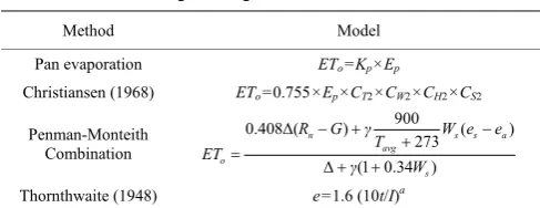
2.4 Evapotranspiration estimation

Evapotranspiration is one of the most basic components of the hydrologic cycle. It denotes the quantity of water transpired by plants plus the moisture evaporated from the surface of the soil and the vegetation (Adamala et al., 2014b,c). Table 2 shows the different evapotranspiration estimation methods that were included in the Hydrologic Calculator software.

Table 2 Evapotranspiration estimation methods

Method Model

Pan evaporation ETo=Kp×Ep

Christiansen (1968) ETo=0.755×Ep×CT2×CW2×CH2×CS2

Penman-Monteith Combination

900

0.408Δ( ) ( )

273

Δ (1 0.34 )

n s s a

avg o

s

R G γ W e e

T ET γ W − + − + = + + Thornthwaite (1948) e=1.6 (10t/I)a

Note: ETo = reference crop evapotranspiration (mm); Kp = pan coefficient; Ep = pan evaporation (mm day-1_{); e = unadjusted potential evapotranspiration, cm per}

month; t = mean air temperature (ºC); I = annual or seasonal heat index, the summation of 12 values of monthly heat indices (i) when, i = (t/5)1.514, a = an empirical exponent; CT2, CW2, CH2, CS2 = empirical constants; Rn = daily net solar radiation (MJ m-2 _day-1_{); G = soil heat flux (MJ m}-2 _day-1_{); e}

s = saturation vapor pressure (kPa); ea = actual vapor pressure (kPa); Δ = slope of saturation vapor pressure versus air temperature curve (kPa ºC-1_{); T}

avg = average daily air temperature at 2 m height (ºC); Ws = wind speed at 2 m height (m s-1); γ = psychrometric constant (kPa ºC-1).

2.5 Infiltration models

Infiltration is the process of the entry of water into a

soil through the soil surface in a vertically downward direction. Infiltration rate (f) is the rate at which water enters the soil surface. Table 3 shows the different infiltration models that were included in the Hydrologic Calculator software.

Table 3 Infiltration estimation methods

Method Model

Kostiakov _{f=( ).ab t}b−1

Green-Ampt (GA) f K aK

F

= +

Phillip Two-Term _{( / 2)}0.5 0.5

c

f₌ a t− ₊f

Horton f =fc+(f0−fc)exp( )−at

Note: K = Darcy’s hydraulic conductivity; F = cumulative infiltration capacity;

f = infiltration rate at any time t from the start of the rainfall; f0 = initial

infiltration rate at t = 0; fc = final steady state infiltration rate occurring at t = tc; a and b = local parameters with a>0 and 0<b<1.

3 Hydrologic Calculator software interface

The Visual Basic 6.0 programming language is used to develop the software, called Hydrologic Calculator. The Hydrologic Calculator interface was developed with a total of eight modules. Figure 1 and Figure 2 show the block diagram and main menu window of the developed software, respectively with different modules and sub-modules. Module-I was designed for analyzing rainfall records with sub-modules to test the consistency of rainfall records, to estimate missing data (using simple average, normal ratio, inverse square distance, and linear programming methods), to estimate mean rainfall (using average, two-axis, finite element, and Thiessen polygon), representation of rainfall data (mass curve and hyetograph), and to test the adequacy of raingauge stations. Module-II facilitates the analysis of runoff using

φ-index, rational, velocity-area, and SCS-CN methods. Module-III includes four sub-modules for estimation of unit hydrograph (UH) from direct runoff hydrograph (DRH) and flood hydrograph (FH), construction of FH from DRH and UH, deriving UH of different durations (method of superposition and S-curve), construction of Synthetic UH (Snyder's method and Triangular hydrograph).

serial correlation and turning point test), and frequency analysis (empirical and frequency factor methods). Module VI and VII facilitate evapotranspiration (Pan evaporation, Christiansen pan evaporation, Penman- Monteith, and Thornthwaite methods) and infiltration (Kostiakov, Green-Ampt, Philip Two-term, and Horton

models) analysis, respectively. Module VIII analyzes the stage-discharge relationships using the rating curve method. To facilitate classroom usage, a comprehensive ‘Help’ module is also provided in the Hydrologic Calculator with a set of basic theory and methodologies of different hydrological processes.

Figure 2 Main menu window of the developed software

4 Validation of Hydrologic Calculator

The Hydrologic Calculator software includes a graphical user interface (GUI) that allows the user to select and edit data, save and retrieve input and output data files, and to view the output both in graphical (line and bar) and tabular forms. The Hydrologic Calculator was tested against the solved numerical solutions from different published books (Table 1). Wherever, solved numerical were not available, the software was tested against the hand calculations. One of the very important aspects of Hydrologic Calculator is logging of the stepwise calculations for all designed modules. The user can save step wise calculations in to a log file (.txt).

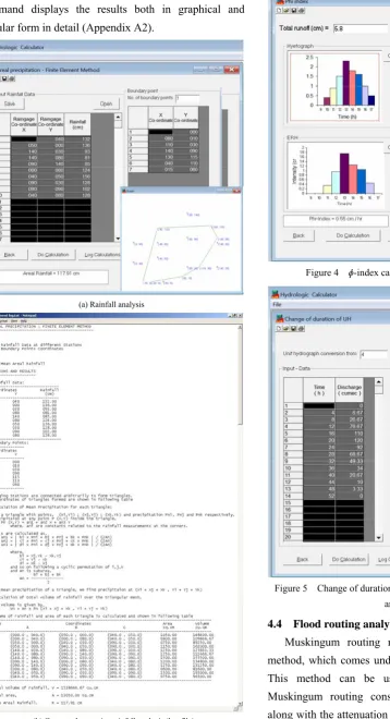
4.1 Rainfall analysis

The point rainfall can be converted to areal rainfall using methods described in the ‘rainfall analysis’ module of Figure 1. Figure 3a shows the data input window as well as results for the Finite Element method. In the case of Finite Element method, the user has to enter point rainfall values for all the stations in the spreadsheet of the active window along with the (x,y) coordinates of raingauge stations as well as coordinates for the watershed boundary. The (x,y) coordinates of raingauge stations and watershed boundary are also displayed in a graphical form (Figure 3a). The ‘Do calculation’ command performs the analysis and displays mean areal rainfall. To save the step wise calculations in a log file (.txt), the user has to click Log Calculations button (Figure 3b).

Similar type of windows were developed for checking the consistency of rainfall records (double mass curve and VNR methods), to estimate missing data (using simple average, normal ratio, inverse square distance, and linear programming methods), to estimate mean areal rainfall (using average, two-axis, and Thiessen polygon), interpretation of rainfall data (mass curve and hyetograph), and to test the adequacy of raingauge stations. The results pertaining to above analysis are not shown and discussed due to space limitations.

4.2 Runoff analysis

In order to calculate the φ -index, the analysis window (Figure 4) can be assessed by clicking on the Runoff analysis module (Figure 2). The active window contains a spreadsheet for entering information on rainfall intensity at different time scale. Further, the user also has to specify the total runoff depth (cm). After entering the required data, select the number of rows to be considered for calculation and press on the 'Do Calculation' button to obtain the φ-index (cm h-1) value and effective rainfall duration (h). The model also provides a graphical display of effective rainfall hyetograph (ERH) and rainfall hyetograph. The stepwise procedure for calculating φ-index is shown in Appendix A1 as log file (.txt).

4.3 Hydrograph analysis

(discharge and time) for a given UH as well as the duration of old and new UHs. The 'Do Calculation' command displays the results both in graphical and Tabular form in detail (Appendix A2).

(a) Rainfall analysis

(b) Generated step wise rainfall analysis (log file) Figure 3 Rainfall analysis and generated step wise rainfall

analysis using Finite Element method

Figure 4 ɸ-index calculation in runoff analysis

Figure 5 Change of duration of unit hydrograph in hydrograph analysis

4.4 Flood routing analysis

routing' module (Figure 6). In this method, the user has to enter information on inflow hydrograph (time and inflow discharge) along with the outflow discharge. Appendix A3 shows a detailed stepwise analysis window for the estimation of coefficient k and x in Muskingum equation.

Figure 6 Determination of constants in hydrological Muskingum routing method

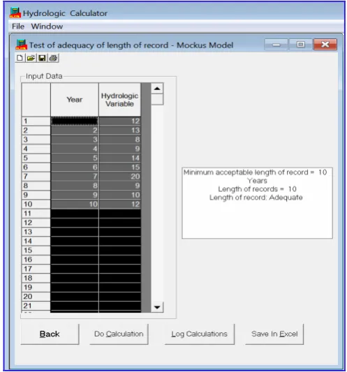
4.5 Frequency analysis

The frequency analysis can be done either using the empirical methods or frequency factor methods. However, prior to applying any of these methods, the data should be tested for adequacy of the length of record and randomness. To test the adequacy of the length of record, the analysis window can be assessed by clicking on ‘Statistical Analysis’ module (Figure 7). In this method, the user has to enter the values of the hydrologic variable in the spreadsheet. The model tests the input data series for adequacy of the length of the record using the Mockus model and displays the results in developed module. 4.6 Evapotranspiration estimation

To estimate the evapotranspiration using the Thornthwaite method, the input window can be opened by clicking on the ‘evapotranspiration analysis’ module (Figure 8). In the input window, a spreadsheet is displayed to enter the mean monthly temperature and mean sunshine hours for each month. Potential evapotranspiration (PET) values can be obtained by clicking on the 'Do Calculation' button. Stepwise calculations can be saved in a log file (.txt) by clicking on the Log Calculations button (Appendix A4).

Figure 7 Testing adequacy of length of records using Mockus model

Figure 8 Evapotranspiration estimation using Thornthwaite method

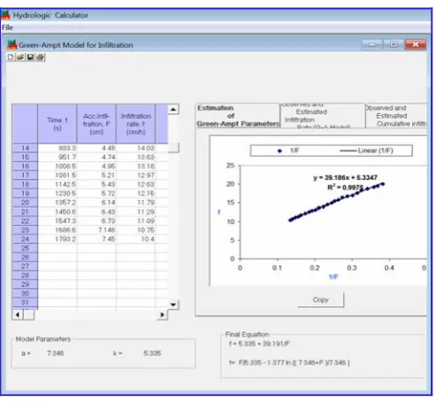
4.7 Infiltration estimation

displayed (Figure 9). Stepwise calculations can be saved in a log file (.txt) by clicking on the ‘log calculations’ button (Appendix A5).

Figure 9 Estimation of Green-Ampt parameters

4.8 Stage-discharge analysis

Rating curve is a relationship between the gauge height and discharge, and is used for estimating the discharge corresponding to known gauge height. To calculate discharge at particular gauge height, the analysis window can be assessed by clicking on the ‘stage-discharge analysis’ module. Figure 10 shows the results related to rating curve analysis. The detailed generated stepwise procedure for analyzing the rating curve is shown in Appendix A6. Inside the active window, input data frame contains a spreadsheet for entering the data related to gauge height and discharge. The user has to specify the value of gauge height at zero discharge. The output contains information on the coefficient of correlation and graphical representation of rating curve. In case the user does not know the gauge height at zero discharge, the model asks for a permission to calculate it. Once the calculation is over, the user is able to calculate discharge for different gauge heights.

Similar types of windows were developed for different sub-modules of runoff, hydrograph, flood routing, frequency analysis, evapotranspiration and infiltration estimation, and stage-discharge relationships. Due to the similarity in analyzing these hydrological processes, the developed windows are not shown here. Further, the software is equipped with a help file for

user’s reference. The help file contains the detailed information on the step by step procedure of working of software.

A pilot validation study was conducted from under graduation and research students of various institutes in India and one institute in Nepal to determine the effectiveness of the Hydrologic Calculator tool in solving and simulating hydrological processes. Several suggestions were welcomed from the participants during this validation and efforts are always made to improve this tool. Hydrologic Calculator was effective in facilitating students’ learning and understanding of hydrologic concepts. Thus, the software is validated successfully and can be used as a professional tool to teach and analyze various hydrological processes.

Figure 10 Stage-discharge analysis using Rating curve method

5 Conclusions

data. The model covers different techniques for analysis of hydrologic data dealing with rainfall, runoff, hydrograph, flood routing, frequency analysis, evapotranspiration estimation, infiltration models, and stage-discharge analysis. For each analysis, the model provides several options to the user. Furthermore, the model includes GUI and a system to store the result in a local file system. The important property of the GUI is that it allows user to select a particular method among various available methods for a given analysis, edit, and retrieve input data, and display of results both in table or graphical forms. It also allows the user to save the step wise calculations in a log file (.txt format). The “Hydrologic Calculator” also saves the step-wise calculation of the problems and thus the print of the file can be taken and used as a guideline. The graphs, etc. can be copied and can be saved in bmp/gif/jpg format.

The completed methods of “Hydrologic Calculator” model were validated or tested with the help of standard examples from different textbooks. The results obtained using the Hydrologic Calculator matched exactly with the respective results given in the source. Thus, it can be concluded that the “Hydrologic Calculator” model is validated successfully and can be used to perform rainfall, runoff, hydrograph, flood routing, statistical analysis, evapotranspiration estimation, infiltration models analysis, and rating curve analysis. The adaptability of this software will make teaching and learning of basic hydrology more interesting and stimulating. Further, it will prove a good analytical tool for field engineers. The software will have a wide application in both teaching and research in the several disciplines related to water and the environment.

Abbreviations

Abbreviation Full title

WHAT Web GIS based Hydrograph Analysis Tool WBNM Watershed Bounded Network Model

IHACRES Identification of unit Hydrographs And Component flows _{from Rainfall, Evaporation and Stream-flow data}

HEC-SSP Hydrologic Engineering Center-Statistical Software Package RRL Rainfall Runoff Library

UH Unit Hydrograph DRH Direct Runoff Hydrograph

FH Flood Hydrograph ISD Inverse Square Distance

Appendix

A1: Calculation of Phi-index and effective rainfall

hyetograph

GIVEN: ---

(1) Total Runoff, R (cm)

(2) Rainfall Intensity vs Time data,

Intensity in cm h-1 and time in (hh:mm) TO FIND:

---

(1) Phi-Index (cm h-1)

(2) Effective Rainfall Hyetograph, ERH (Intensity vs Time) CALCULATIONS AND RESULTS: ---

(1) Total Runoff = 5.8 cm

(2) Time distribution of the storm:

Time (h) Incremental Rainfall (cm)

09.00 00.00 10.00 00.40 11.00 00.90 12.00 01.50 13.00 02.30 14.00 01.80 15.00 01.60 16.00 01.00 17.00 00.50

Time Interval (h) Rainfall (cm)

01.00 00.00 01.00 00.40 01.00 00.90 01.00 01.50 01.00 02.30 01.00 01.80 01.00 01.60 01.00 01.00

(3) Total Infiltration = 9.5 – 5.8 = 3.7

(4) Assume te = time of rainfall excess = 8 hr for the first trial

Hence,

3.7

Phi 0.4625

8

= =

Time = 9 hr and Magnitude = 0 cm Time = 10 hr and Magnitude = 0.4 cm

(5) Subtracting above rainfall(s) and modifying the value of te

Now te = 6 hr Therefore,

3.3

Phi 0.55

6

= =

Hence, Phi-Index = 0.55 cm h-1

Rainfall Excess Duration = 6 hr

A2: Changing the duration of a unit hydrograph GIVEN:

---

(1) Duration of the original UH (D hr)

(2) Duration of the required UH (t hr) (3) Ordinates of the original UH CALCULATIONS AND RESULTS: ---

S Curve Method Steps:

(1) D = 4 hr (2) t = 12 hr

(3) Develop D hr (4 hr) S-Curve using standard technique (col.4)

(4) Develop another D-hr (4 hr) S-Curve lagged by t hr (12 hr) from the first one (col.5)

(5) Ordinate (Sa - Sb) represents a DRH by t hr (12 hr) effective rainfall and t/D (3)magnitude (col.6) (6) t hr (12 hr) UH = ((Sa - Sb) × D)/t (col.7)

Time (hr)

4 hr UH ordinates (cumec)

S-Curve addition (cumec)

S-Curve ordinate (cumec) (2) + (3)

S-Curve lagged by 12 hr (cumec)

Sa - Sb (4) - (5)

12 hr UH ordinates (cumec) (6)/(t/D)

(1) (2) (3) (4) (5) (6) (7)

000 000.00 000.00 000.00 000.00 000.00 000.00

004 020.00 000.00 020.00 000.00 020.00 006.67

008 060.00 020.00 080.00 000.00 080.00 026.67

012 150.00 060.00 230.00 000.00 230.00 076.67

016 120.00 150.00 350.00 020.00 330.00 110.00

020 090.00 120.00 440.00 080.00 360.00 120.00

024 066.00 090.00 506.00 230.00 276.00 092.00

028 050.00 066.00 556.00 350.00 206.00 068.67

032 032.00 050.00 588.00 440.00 148.00 049.33

036 020.00 032.00 608.00 506.00 102.00 034.00

040 010.00 020.00 618.00 556.00 062.00 020.67

044 000.00 010.00 618.00 588.00 030.00 010.00

048 000.00 000.00 618.00 608.00 010.00 003.33

052 000.00 000.00 618.00 618.00 000.00 000.00

A3: Hydrologic flood routing: determination of

Muskingum coefficients k and x GIVEN:

---

(1) Inflow Hydrograph (2) Outflow Hydrograph

TO FIND: ---

Muskinghum Equation Coefficients: (1) K

(2) x

CALCULATIONS AND RESULTS:

Time (hr)

Inflow I (cumec)

Outflow Q (cumec)

I-Q (cumec)

Average I-Q (cumec)

delta S (5) × delta t (cumec hour)

Storage S Cumulative (6) (cumec hour)

(1) (2) (3) (4) (5) (6) (7)

00 05.00 05.00 000.00 000.00 000.00 000.00

06 20.00 06.00 014.00 007.00 042.00 042.00

12 50.00 12.00 038.00 026.00 156.00 198.00

18 50.00 29.00 021.00 029.50 177.00 375.00

24 32.00 38.00 –006.00 007.50 045.00 420.00

30 22.00 35.00 –013.00 –009.50 –057.00 363.00

36 15.00 29.00 –014.00 –013.50 –081.00 282.00

42 10.00 23.00 –013.00 –013.50 –081.00 201.00

48 07.00 17.00 –010.00 –011.50 –069.00 132.00

54 05.00 13.00 –008.00 –009.00 –054.00 078.00

60 05.00 09.00 –004.00 –006.00 –036.00 042.00

[x.I + (1–x).Q] (cumec)

x=0.00 x=0.02 x=0.04 x=0.06 x=0.08 x=0.10 x=0.12 x=0.14 x=0.16 x=0.18 x=0.20 x=0.22 x=0.24 x=0.26 x=0.28 x=0.30

05.0 05.0 05.0 05.0 05.0 05.0 05.0 05.0 05.0 05.0 05.0 05.0 05.0 05.0 05.0 05.0 06.0 06.3 06.6 06.8 07.1 07.4 07.7 08.0 08.2 08.5 08.8 09.1 09.4 09.6 09.9 10.2 12.0 12.8 13.5 14.3 15.0 15.8 16.6 17.3 18.1 18.8 19.6 20.4 21.1 21.9 22.6 23.4 29.0 29.4 29.8 30.3 30.7 31.1 31.5 31.9 32.4 32.8 33.2 33.6 34.0 34.5 34.9 35.3 38.0 37.9 37.8 37.6 37.5 37.4 37.3 37.2 37.0 36.9 36.8 36.7 36.6 36.4 36.3 36.2 35.0 34.7 34.5 34.2 34.0 33.7 33.4 33.2 32.9 32.7 32.4 32.1 31.9 31.6 31.4 31.1 29.0 28.7 28.4 28.2 27.9 27.6 27.3 27.0 26.8 26.5 26.2 25.9 25.6 25.4 25.1 24.8 23.0 22.7 22.5 22.2 22.0 21.7 21.4 21.2 20.9 20.7 20.4 20.1 19.9 19.6 19.4 19.1 17.0 16.8 16.6 16.4 16.2 16.0 15.8 15.6 15.4 15.2 15.0 14.8 14.6 14.4 14.2 14.0 13.0 12.8 12.7 12.5 12.4 12.2 12.0 11.9 11.7 11.6 11.4 11.2 11.1 10.9 10.8 10.6 09.0 08.9 08.8 08.8 08.7 08.6 08.5 08.4 08.4 08.3 08.2 08.1 08.0 08.0 07.9 07.8 07.0 07.0 06.9 06.9 06.8 06.8 06.8 06.7 06.7 06.6 06.6 06.6 06.5 06.5 06.4 06.4

Plot [x.I + (1–x).Q] vs Storage, S for all values of x Choose that value of x which gives the thinnest loop i.e close to a straight line

Fit a straight line through points for above value of x Inverse slope of the straight line will give the value of K

Here,

x = 0.2

K = 13.3 hours

A4: Thornthwaite evapotranspiration calculation

Given: (1) Mean monthly Temperatures in degree Celsius. (t)

(2) Mean monthly Sunshine Hours. (h) Formulae Used:

(1) Monthly Heat Index,

i = (t/5)^1.514

(2) Annual or Seasonal heat index, I = sum of all i's

(3) An empirical exponent,

a = 0.000000675 x I^3 – 0.0000771 x I^2 + 0.01792 x I +0.49239

(4) Unadjusted Potential Evapotranspiration (in cm),

e = 1.6(10 t/I)^a (5) Correction Factor,

c = (sunshine hours x no. of days in month) / (12 × 30)

(6) Corrected Potential Evapotranspiration (in cm),

pet = e × c

(7) Total Potential Evapotranspiration (in cm), PET = sum of all pet’s

Mean Monthly Temperature (deg. C)

(t)

Mean Monthly Sunshine Hours (hours)

(h)

Monthly Heat Index (i) (t/5)^1.514

Unadjusted PET (cm) (e) 1.6(10t/I)^a

Correction (c) (h*days)/(12*30)

CorrectedValues of PET (cm)

(e*c)

12.60 10.60 4.052 1.387 0.913 1.266

15.80 11.20 5.709 2.777 0.871 2.419

20.70 12.00 8.593 6.359 1.033 6.571

27.00 12.80 12.848 14.364 1.067 15.322

31.10 13.60 15.915 22.161 1.171 25.953

33.50 13.90 17.811 27.835 1.158 32.243

30.60 13.80 15.529 21.086 1.188 25.057

29.00 13.10 14.316 17.884 1.128 20.174

28.20 12.40 13.723 16.414 1.033 16.961

24.80 11.40 11.297 11.068 0.982 10.865

18.90 10.80 7.487 4.811 0.900 4.330

13.70 10.30 4.600 1.793 0.887 1.591

I = 132 PET = 162.752

A5: Infiltration model: Green-Ampt model GIVEN:

---

(1) Infiltration Measurements (Infiltration depth and rate vs time)

TO FIND: ---

(1) Green-Ampt Model Parameters K and a (2) Green-Ampt Model Equation for Infiltration CALCULATIONS AND RESULTS

---

(1) Green-Ampt Model is expressed as

a

f K K

F

= + −

ln

F a f

t C

K a

+

⎛ ⎞

= _{⎜ ⎟}+

⎝ ⎠

where, K and a are model parameters; F is infiltration depth; f is infiltration rate; C is constant of integration. (2) Relationship between f and F is:

a

f K K

F

= + −

(3) Plotting graph of f vs F and fitting a straight line, K is given by the y intercept and K.a is given by the slope

(4) Calculations:

Time t (min)

Accumulated Infiltration

F (cm)

Infiltration Rate

f (cm h-1₎

1/F F (Model)

(cm) f (Model) (cm h-1₎

0472.2 02.62 20.02 00.38 02.52 20.29

0489.7 02.72 19.54 00.37 02.62 19.74

0507.5 02.80 19.21 00.36 02.72 19.33

0531.5 02.94 18.75 00.34 02.85 18.66

0559.8 03.08 18.32 00.32 03.00 18.06

0582.3 03.19 17.60 00.31 03.11 17.62

0609.4 03.32 17.00 00.30 03.25 17.14

0644.1 03.48 16.70 00.29 03.41 16.60

0682.9 03.66 16.42 00.27 03.59 16.04

0714.7 03.80 15.74 00.26 03.73 15.65

0751.1 03.95 15.43 00.25 03.89 15.26

0783.9 04.09 14.93 00.24 04.03 14.92

0831.2 04.28 14.46 00.23 04.22 14.49

0883.3 04.48 14.03 00.22 04.43 14.08

0951.7 04.74 13.63 00.21 04.70 13.60

1008.5 04.95 13.18 00.20 04.91 13.25

1081.5 05.21 12.97 00.19 05.17 12.86

1142.5 05.43 12.63 00.18 05.39 12.55

1230.5 05.72 12.15 00.17 05.69 12.19

1357.2 06.14 11.79 00.16 06.12 11.72

1450.6 06.43 11.29 00.16 06.42 11.43

1547.3 06.73 11.09 00.15 06.72 11.16

1686.6 07.15 10.75 00.14 07.15 10.82

1793.2 07.45 10.40 00.13 07.46 10.59

(5) From step 3, we get, K = 5.33473 K.a = 39.186 or, a = 7.346

(6) Green-Ampt Model Parameters: K = 5.335

a = 7.346

(7) Green-Ampt Model Equation: f = 5.335 + 39.191/F

t = F/5.335 – 1.377 ln [(7.346+F)/7.346]

A6: Stage-discharge relationship: Rating curve

method

GIVEN: ---

(1) Gauge Height for zero discharge, a (m) [optional]

(2) Gauge Reading (Stage) vs Discharge data Stage in m and Discharge in cumec (3) Gauge Reading at which discharge to be calculated, G (m) [optional]

TO FIND: ---

(1) Stage - Discharge Relationship (2) Coefficient of Correlation

(3) Gauge Height for zero discharge, a (m) [if required]

CALCULATIONS AND RESULTS ---

(1) Gauge Height for zero discharge, a = 7.50 m (2) Input: First two columns of the table. (3) The gauge - discharge equation is:

Q = Cr.(G – a)^beta (1) where, Q is stream discharge; G is gauge height (stage); a is gauge Height for zero discharge; Cr and beta are rating curve constants.

By taking logarithms of eqn (1) log Q = beta . log (G–a) + log Cr or Y = beta . X + b

where, Y = log Q and X = log(G–a).

Gauge G (m)

Discharge Q (cumec) (G-a)

X = log(G-a)

Y = log Q

(XY) (cumec)

07.65 0015.00 00.15 –0.824 1.176 –0.969 07.70 0030.00 00.20 –0.699 1.477 –1.032 07.77 0057.00 00.27 –0.569 1.756 –0.998 07.80 0039.00 00.30 –0.523 1.591 –0.832 07.90 0060.00 00.40 –0.398 1.778 –0.708 07.91 0100.00 00.41 –0.387 2.000 –0.774 08.08 0150.00 00.58 –0.237 2.176 –0.515 08.48 0180.00 00.98 –0.009 2.255 –0.020 08.98 0280.00 01.48 0.170 2.447 0.417 09.30 0550.00 01.80 0.255 2.740 0.700 09.50 0970.00 02.00 0.301 2.987 0.899 10.50 1900.00 03.00 0.477 3.279 1.564 11.10 1600.00 03.60 0.556 3.204 1.782 11.70 1200.00 04.20 0.623 3.079 1.919

(4) From the above table,

sum (X) = –1.2611 sum (Y) = 31.9460 sum (XY) = 1.4337

sum (X2) = 3.2382 sum (Y2) = 79.0801 (sum (X))2 = 1.5903 (sum (Y))2 = 1020.5478 (5) Now, from regression line,

2 2

. ( ) ( ). ( )

. ( ) ( ( ))

(14 1.434) ( 1.261)(31.946)

1.380

(14 3.238) 1.590

N sum XY sum X Sum Y

beta

N sum X Sum X

− =

−

× − −

= =

× −

sum(Y) – beta.sum(X)

( ) . ( )

(31.9460142757761) 1.380( 1.261)

2.406

14

sum Y beta sum X

b

N − =

− −

= =

Hence,

Cr = 254.769

(6) The required gauge-discharge relationship is therefore

Q = 254.8(G-a)^1.380 (7) Coefficient of correlation,

2 2 2 2

. ( ) ( ( ))( ( ))

[ . ( ) ( ( )) ][ . ( ) ( ( )) ]

0.981

N sum XY sum X sum Y

r

N sum X sum X N sum Y sum Y

− =

− −

=

The value of r is be close to 1.

References

Adamala, S., N. S. Raghuwanshi, and A. Mishra. 2014a. Development of surface irrigation systems design and evaluation software (SIDES). Computers and Electronics in Agriculture, 100C: 100–109.

Adamala, S., N. S. Raghuwanshi, A. Mishra, and M. K. Tiwari.

2014b. Evapotranspiration modeling using second-order neural networks. Journal of Hydrologic Engineering, 19(6): 1131–1140.

Adamala, S., N. S. Raghuwanshi, A. Mishra, and M. K. Tiwari. 2014c. Development of generalized higher-order synaptic neural-based ETo Models for different agroecological regions

in India. Journal of Irrigation and Drainage Engineering, 140(12): 04014038.

Akin, J. E. 1971. Calculation of the mean areal depth of precipitation. Journal of Hydrology, 12(4): 363–376.

Allen, G. R., and G. Liu. 2011. IHACRES Classic: Software for the identification of unit hydrographs and component flows. Ground Water, 49(3): 305–308.

ASCE. 1990. Perspective on water resources education and training. Journal of Water Resources Planning and Management, 116(1): 99–133.

Bandyopadhyaya, A., A. Bhadra, R. K. Swarnakar, N. S. Raghuwanshi, and R. Singh. 2012. Estimation of reference evapotranspiration using a user-friendly decision support system: DSS_ET. Agricultural and Forest Meteorology, 154-155: 19–29.

Bethlahmy, N. 1976. The two-axis method: A new method to calculate average precipitation over a basin. International Association of Scientific Hydrology Bulletin, 21(3): 379–385. Bourget, P. G. 2006. Integrated water resources management

curriculum in the United States: results of a recent survey. Journal of Contemporary Water Research and Education, 135: 107–114.

Boyd, M. J., E. H. Rigby, and R. Van Drie. 1996. WBNM – a computer software package for flood hydrograph studies. Environmental Software, 11(1-3): 167–172.

Christiansen, J. E. 1968. Pan evaporation and evapotranspiration form climatic data. Journal of the Irrigation and Drainage Division, 94(2): 243–265.

Chow, V. T., D. R. Maidment, and L. W. Mays. 1988. Applied Hydrology. New York: McGraw-Hill.

CUAHSI. 2010. Water in a dynamic planet: A five-year strategic plan for water science. Washington, D.C., doi:10.4211/sciplan.200711.

Harris, J., G. Brunner, M. Fleming, and B. Faber. 2010. Statistical software package. In 2nd _{Joint Federal Interagency}

Conference, pp.5. Davis CA: US Army Corps of Engineers, Hydrologic Engineering Center.

Habib, E., Y. Ma, D. Williams, H. O. Sharif, and F. Hossain. 2012. HydroViz: Design and evaluation of a Web-based tool for improving hydrology education. Hydrology and Earth System Sciences, 16: 3767–3781.

Howe, C. W. 2008. Preface to a creative critique on U.S. water education. Journal of Contemporary Water Research and Education, 139: 1–2.

Recommendations for making geoscience data accessible and usable in education. Eos, Transactions American Geophysical Union, 89(32): p 291.

Lim, K. J., B. A. Engel, Z. Tang, J. Choi, K. S. Kim, S. Muthukrishnan, and D. Tripathy. 2005. Automated web GIS based hydrograph analysis tool, WHAT. JAWRA Journal of the American Water Resources Association, 41(6): 1407–1416.

Loucks, D. P. 2008. Educating future water resources managers. Journal of Contemporary Water Research and Education, 139: 17–22.

MacDonald, L. H. 1993. Developing a field component in hydrologic education. Journal of American Water Resources Association, 29(3): 357–368.

Merwade, V. and B. L. Ruddell. 2012. Moving university hydrology education forward with community-based geoinformatics, data and modeling resource. Hydrology and Earth System Sciences, 16: 2393–2404.

Michael, A. M. 2009. Irrigation: Theory and Practice. New Delhi: Vikas Publishing House.

Mockus, V. 1960. Selecting a flood frequency method. American Society of Agricultural and Biological Engineers, 3(1): 48–51. Nash, J. E., P. S. Eagleson, J. R. Philip, W. H. van der Molen, V.

and V. Klemes. 1990. The education of hydrologists (Report of an IAHS/UNESCO Panel on hydrological education). Hydrological Sciences, 35(6): 597–607.

Ngambeki, I., S. E. Thompson, P. A. Troch, M. Sivapalan, and D. Evangelou. 2012. Engaging the students of today and preparing the catchment hydrologists of tomorrow: Student-centered approaches in hydrology education. Hydrology and Earth System Sciences, 9(1): 707–740.

Pathirana, A., J. H. Koster, E. de Jong, and S. Uhlenbrook. 2012. On teaching styles of water educators and the impact of didactic training. Hydrology and Earth System Sciences, 16(10): 3677–3688.

Perraud, J. M., G. M. Podger, J. M. Rahman, and R. A. Vertessy. 2003. A new rainfall-runoff software library. Proceedings of

Modelling and Simulation (MODSIM), 4: 1733–1738.

Raes, D., P. Willems, and F. G. Baguidi. 2006. RAINBOW–a software package for analyzing data and testing the homogeneity of historical data sets. In Proceedings of the 4th

International Workshop on ‘Sustainable Management of Marginal Drylands, 27–31. Islamabad, Pakistan: 27-31 January 2006.

Ruddell, B. L., and T. Wagener. 2013. Grand challenges for hydrology education in the 21st _{century. Journal of Hydrologic}

Engineering, 20(1): A4014001.

Sanchez, C. A., B. L. Ruddell, R. Schiesser, and V. Merwade. 2015. Enhancing the T-shaped learning profile when teaching hydrology using data, modeling, and visualization activities. Hydrology and Earth System Sciences, 12: 6327–6350. Seibert, J., S. Uhlenbrook, and T. Wagener. 2013. Hydrology

education in a changing world. Hydrology and Earth System Sciences, 17(4): 1393–1399.

Singh, V. P. 1994. Elementary Hydrology. New Delhi: Prentice Hall of India-Private Limited.

Subramanya, K. 2013. Engineering Hydrology. New Delhi: Tata McGraw-Hill Publishing Company Limited.

Suresh, R. 2013. Soil and Water Conservation Engineering. New Delhi: Standard Publishers Distributors.

Thornthwaite, C. W. 1948. An approach towards a rational classification of climate. Geographical Review, 38(1): 55–94. Uhlenbrook, S. and E. D. Jong. 2012. T-shaped competency

profile for water professionals of the future. Hydrology and Earth System Sciences, 16(10): 3475–3483.

Wagener, T., C. Kelleher, M. Weiler, B. McGlynn, M. Gooseff, L. Marshall, and S. Zappe. 2012. It takes a community to raise a hydrologist: the Modular Curriculum for Hydrologic Advancement (MOCHA). Hydrology and Earth System Sciences, 16: 3405–3418.