Int. J. IndustrialMathematics (ISSN 2008-5621) Vol. 6, No. 3, 2014 Article ID IJIM-00504, 9 pages
Research Article
The Ritz-Galerkin method for MHD Couette flow of non-Newtonian
fluid
Z. Barikbin ∗, R. Ellahi †, S. Abbasbandy‡§
————————————————————————————————–
Abstract
In this paper, the Ritz-Galerkin method in Bernstein polynomial basis is applied for solving the nonlinear problem of the magnetohydrodynamic (MHD) flow of third grade fluid between the two plates. The properties of the Bernstein polynomials together with the Ritz-Galerkin method are used to reduce the solution of the MHD Couette flow of non-Newtonian fluid in a porous medium to the solution of algebraic equations.
Keywords: Ritz-Galerkin method; Bernstein polynomials; Satisfier function; MHD.
—————————————————————————————————–
1
Literature review
N
omost important subjects in modern appliedn-Newtonian fluid dynamics is one of the mathematics. This is due to the fact that non-Newtonian fluids are of considerable inter-est in many industrial and technological applica-tions. In nature there are different kinds of non-Newtonian fluids. All such fluid in terms of their diverse characteristics cannot be described by one constitutive equation. Hence different fluid mod-els have been proposed. Amongst these a subclass of differential type fluids third grade can predict the shear thinning/shear thickening effects even in steady unidirectional flow over rigid boundary. MHD consideration of non-Newtonian fluids is important in the metallurgical process. Further,∗Department of Mathematics, Imam Khomeini
Inter-national University, Ghazvin, 34149, Iran.
†Department of Mathematics & Statistics, Faculty of
Basic and Applied Sciences, International Islamic Univer-sity, Islamabad, Pakistan.
‡Corresponding author. [email protected] §Department of Mathematics, Imam Khomeini
Inter-national University, Ghazvin, 34149, Iran.
the non-Newtonian fluids in porous media are en-countered in fields like ceramics production, cer-tain separation processes, filtration and oil recov-ery, petroleum production, food processing, poly-mer engineering etc. Having such importance of non-Newtonian fluids in mind, many researchers are engaged to examine various physical aspects of such fluids in different flow figurations (see for instance the studies [1, 2, 3, 4, 5, 6, 7, 8, 9, 10] and many references therein).
Recently, the effects of nonlinear partial slip on the walls for steady flow and heat transfer of an incompressible, thermodynamically compati-ble third grade fluid in a channel is investigated in [11]. In that paper, the space between two plates is not a porous media and the upper plate is moving with uniform velocity.
The Ritz method is a variational method. Vari-ational methods are approximate methods for the solutions of boundary value problems (BVP). These methods include the Collocation, Galerkin (with its various versions [12]), least squares methods and the moment methods; amongst oth-ers. In each variational algorithm, we obtain some Coefficients of some given assumed
imate solutions to the BVP that would satisfy Some boundary given conditions. In this paper, the Ritz-Galerkin method in Bernstein polyno-mial basis is used. The approximation of the problem is based on the modified Bernstein nomial basis. The properties of Bernstein nomials are first presented. The Bernstein poly-nomial basis vanish except the first polypoly-nomial at
x = 0, which is equal to 1 and the last polyno-mial at x= R, which is also equal to 1 over the interval [0, R]. This provides greater flexibility in which to impose boundary conditions at the end points of the interval.
In this work, Couette flow of an incompress-ible third grade fluid is considered. The fluid is electrical conducted in the presence of uniform applied magnetic field B0 in the y-direction. In-duced magnetic field is not taken into account in view of small magnetic Reynolds number. The fluid saturates the porous space between two infi-nite plates. The lower plate aty= 0 is stationary while the upper plate aty =his suddenly jerked with the velocityU0. Slip effects in terms of shear stress is considered. For unidirectional steady flow, the velocity field V = (u(y),0,0)) satisfies the incompressibility conditions and equation of motion in absence of axial pressure gradient gives
µd
2u
dy2 + 2β
d dy ( du dy )3 − (1.1) ϕ K [
µ+ 2β
(
du dy
)2]
u−σB02u= 0,
with the subjected boundary conditions
u(0)−γ
[
du dy + 2β
(
du dy
)3]
y=0
= 0, (1.2)
u(2h) +γ
[
du dy + 2β
(
du dy
)3]
y=2h
=U0. (1.3)
In above equations µ is the dynamic viscosity, β
is the material parameter,ϕandkare the poros-ity and permeabilporos-ity of porous medium, σ is the electrical conductivity and γ is the dimensional slip parameter.
At this point, we introduce the following di-mensionless variables
u= u
∗
U0
, y= y
∗
h, γ = γ∗
h,
1
K = h2ϕ
k ,
M = σB 2 0h2
µ , β
∗ = βU02
µh2.
Now dimensionless forms of Eqs. (1.1)-(1.3) are reduced as follows
d2u dy2 + 2β
d dy ( du dy )3 − (1.4) 1 K [
1 + 2β
(
du dy
)2]
u−M u= 0,
with conditions
u(0)−γ
[
du dy + 2β
(
du dy
)3]
y=0
= 0, (1.5)
u(2) +γ
[
du dy + 2β
(
du dy
)3]
y=2
= 1, (1.6)
where asterisks have been suppressed for simplic-ity.
2
Properties of Bernstein
poly-nomials
The general form of the B-polynomials of m th-degree are defined on the interval [0,1] as [13]
Bi,m(x) =
m!
i! (m−i)!x
i(1−x)m−i, 0≤i≤m.
A recursive definition also can be used to generate the B-polynomials over [0,1] so that the ith mth degree B-polynomial can be written
Bi,m(x) = (1−x)Bi,n−1(x) +xBi−1,n−1(x).
It can be readily shown that each of the B-polynomials is positive and also the sum of all the B-polynomials is unity for all real xbelonging to the interval [0,1], that is, ∑mi=0Bi,m(x) = 1. It
can be easily shown that any given polynomial of degree m can be expanded in terms of linear combination of the basis functions
P(x) =
m
∑
i=0
CiBi,m(x), m≥1.
Moreover the Bernstein basis polynomials have the following properties:
i) Bi,m(0) = δi,0and Bi,m(1) = δi,m where δ is
ii) Bi,m(x) has a root with multiplicity i at
point x = 0 (note if i is 0 there is no root at 0).
iii) Bi,m(x) has a root with multiplicity m−i
at pointx = 1 (note if m =i there is no root at 1).
Now suppose that H = L2[0,1] and{B0,m, B1,m, . . . , Bm,m} ⊂ H , be the
set of Bernstein polynomials ofmth degree and:
Y =Span{B0,m, B1,m, . . . , Bm,m}
andf be an arbitrary element inH. SinceY is a finite dimensional vector space, f has the unique best approximation out of Y such asy0 ∈Y, i.e.,
∃y0 ∈Y;∀y∈Y ∥f −y0 ∥≤∥f −y∥.
Since y0 ∈ Y, there exist the unique coefficients
c0, c1, . . . , cm such that:
f ∼=y0=
m
∑
i=0
ciBi,m=cTϕ,
where ϕT = [B0,m, B1,m, . . . , Bm,m] and cT =
[c0, c1, . . . , cm], andcT can be obtained by
cT < ϕ, ϕ >=< f, ϕ >,
in which
< f, ϕ >=
∫ 1
0
f(x)ϕ(x)Tdx= [< f, B0,m>,
, < f, B1,m>, . . . , < f, Bm,m>],
and < ϕ, ϕ > is a (m+ 1)×(m+ 1) matrix and is said dual matrix ofϕ. Let
Q= [Q(i+1),(i+1)] =< ϕ, ϕ >=
∫ 1
0
ϕ(x)ϕ(x)Tdx,
then
cT = (
∫ 1
0
f(x)ϕ(x)Tdx)Q−1.
In the following lemma we present an upper bound to estimate the error.
Lemma 2.1 Suppose that the function g :
[t0, tf] → R is m + 1 times continuously
differentiable, g ∈ Cm+1[t0, tf] and Y =
Span{B0,m, B1,m, . . . , Bm,m}. If cTϕ be the best
approximation of g out ofY then the mean error
bounded is presented as follows
∥g−cTϕ∥≤ M(tf−t0)
(2m+3)/2
(m+ 1)!√2m+ 3,
where M = maxx∈[t0,tf]|g(m+1)(x)|.
Proof. We consider the Taylor polynomial
y1(x) =
g(t0) +g′(t0)(x−t0) +...+g(m)(t0)
(x−t0)m
m! ,
which we know
|g(x)−y1(x)|≤ |g(m+1)(η)|(x−t0)
m+1
(m+ 1)! , (2.7)
where η ∈ (t0, tf). Since cTϕ is the best
approx-imation g out of Y, y1 ∈ Y and using Eq. (2.7) we have
∥g−cTϕ∥22≤∥g−y1 ∥22=
∫ tf
t0
|g(x)−y1(x)|2dx
≤ ∫ tf
t0
[g(m+1)(η)(x−t0)
m+1
(m+ 1)! ] 2dx
≤ M2
(m+ 1)!2
∫ tf
t0
(x−t0)2m+2dx=
M2(tf −t0)2m+3
[(m+ 1)!2](2m+ 3),
and by taking square roots we have the above bound.
3
The Ritz-Galerkin Method
Consider the vector space of real functions whose domain is the closed interval [a, b]. We define the inner product of two functions f(x) and g(x) as follows
< f, g >=
∫ b
a
f(x)g(x)dx.
In this method, we have the following assump-tions:
1)All the functions we use are assumed to be square-integrable.
2) If < f, w >= ∫abf(x)w(x)dx = 0 for any functionw(x), then f(x) = 0.
3) A complete basis for a vector space V of functions is a set of linear independent functions
S ={φi(x)}ii==0∞ which has the property that any
f(x)∈V can be written uniquely as a linear com-bination
f(x) =
∞ ∑
j=0
cjφj(x).
If f(x) ∈ V and < φi, f >= 0 for all φi ∈ S
a finite number of functions{φi(x)}ii==0n.Consider the differential equation
L[y(x)] +f(x) = 0, (3.8)
over the interval a ≤ x ≤ b. The term L[y(x)] denotes a linear differential operator.
Multiplying Eq. (3.8) by any arbitrary weight function w(x) and integrating over the interval [a, b] one obtains
∫ b
a
w(x)(L[y(x)] +f(x))dx= 0, (3.9)
for any arbitraryw(x). The Eqs. (3.8) and (3.9) are equivalent, because w(x) is any arbitrary function.
We introduce a trial solutionu(x) to Eq. (3.8) of the form
u(x) =φ0(x) +
n
∑
j=1
cjφj(x),
and replacey(x) with u(x) on the left side of the Eq. (3.8). The residual is defined as follows
r(x) =L[u(x)] +f(x).
The goal is to construct u(x) so that the inte-gral of the residual will be zero for some choices of weight functions. That is, u(x) will partially satisfy (3.9) in the sense that
∫ b
a
w(x)(L[y(x)] +f(x))dx= 0.
for some choices of w(x) . One of the most important weighted residual methods was intro-duced by the Russian mathematician, Boris Grig-oryevich Galerkin (February 20, 1871 - July 12, 1945). Galerkin’s method selects the weight func-tions in a special way: they are chosen from the basis functions, i.e. w(x) ∈ {φi(x)}ni=1. It is re-quired that the followingn equations hold true
∫ b
a
φi(x)(L[y(x)] +f(x))dx= 0,
fori= 1,2, . . . , n. To apply the method, we solve these n equations for the coefficients {cj}∞j=1. Suppose we wish to solve a boundary value prob-lem over the interval [a, b] with the above method, we select φi(x), i = 1,2, . . . , m so that
sat-isfy the homogeneous form of the specified essen-tial boundary conditions andφ0 must satisfy the specified essential boundary conditions.
4
Solution procedure
By the change of variable
y= 2x,
we get dydu = (1/2)dudx and dyd2u2 = (1/4)d 2u
dx2 then
the Eqs. (1.4)-(1.6) can be written as the differ-ential equation with boundary conditions on in-terval [0,1], i.e.
2d 2u
dx2 +β
d dx
(
du dx
)3 −
1
K
[
8 + 4β
(
du dx
)2]
u−8M u= 0,
with conditions
u(0)−γ
[
(1/2)du
dx+ (1/4)β
(
du dx
)3]
x=0
= 0,
(4.10)
u(1) +γ
[
(1/2)du
dx+ (1/4)β
(
du dx
)3]
x=1
= 1.
(4.11) As y goes from 0 to 2 in the original problem continuously, x goes from 0 to 1 as well in the above differential equation, continuously. Now, having boundary conditions at interval [0,1], we apply Bernstein Ritz-Galerkin method to handle the above problem as follows.
4.1 Satisfier function and
Ritz-Galerkin method
Let
y(x) =
n
∑
i=0
ciϕi(x),
where for arbitrary constantn,ϕi(x) are following
modified Bernstein polynomials:
ϕi(x) =Bi,n, i= 1,2, . . . , n−1,
ϕ0(x) =xB0,n, ϕn(x) = (1−x)Bn,n.
With these choices of polynomials the function
y(x) has the following properties:
y(0) =y(1) = 0, (4.12)
y′(1) =−ncn−1−cn. (4.14)
Let us define the satisfier function ϕ(x) which helps y(x) satisfies conditions (4.10)-(4.11).
Consider the truncated series
¯
u(n)(x) =
n
∑
i=0
ciϕi(x) +ϕ(x) =y(x) +ϕ(x).
The goal is to constructϕ(x) so that ¯u(n)(x) sat-isfies the conditions (4.10)-(4.11).
In general, ϕ(x) is not unique. The simplest choice ofϕ(x) is
ϕ(x) =a+ (3b−3a)x2+ (2a−2b)x3,
such that
a=γ((1/2)(c0+nc1) + (1/4)β(c0+nc1)3),
b=
1−γ((1/2)(−ncn−1−cn)+(1/4)β(−ncn−1−cn)3).
It is worth pointing out that forϕ(x) we have
ϕ′(0) =ϕ′(1) = 0,
ϕ(0) =γ((1/2)(c0+nc1) + (1/4)β(c0+nc1)3),
ϕ(1) =
1−γ((1/2)(−ncn−1−cn)+(1/4)β(−ncn−1−cn)3).
Therefore, by using (4.12)-(4.14), it’s easy to see that ¯u(m)(x) satisfies the conditions (4.10)-(4.11). Now let
F(u) = 2d 2u
dx2 +β
d dx
(
du dx
)3
− (4.15)
1
K
[
8 + 4β
(
du dx
)2]
u−8M u.
For solving (4.15), we approximateu(x) as
u(x)≈u¯(n)(x) =
n
∑
i=0
ciϕi(x) +ϕ(x). (4.16)
Now the expansion coefficientsci are determined
by the Galerkin equations
< F(¯u(n)), Bi,n>= 0, i= 1,2, . . . , n, (4.17)
where< . >denotes the inner product defined by
< F(¯u(n)), Bi,n>=
∫ 1
0
F(¯u(n))(x)Bi,n(x)dx.
Eq. (4.17) gives a system of nonlinear equations which can be solved for the elements of ci using
Newton’s iterative method.
It is important to not that, we made satis-fier function ϕ(x) so that sum of that and trun-cated series ∑ni=0ciϕi(x) is satisfied boundary
conditions. This is different from other Ritz method, where the satisfier function satisfies the each boundary condition.
4.2 Collocation method
By the change of variable
y=x+ 1,
we get dudy = dudx then the problem (1.4)-(1.6) can be written as the differential equation with boundary conditions on interval [−1,1], i.e.,
d2u dx2 + 2β
d dx
(
du dx
)3
− (4.18)
1
K
[
1 + 2β
(
du dx
)2]
u−M u= 0,
with conditions
u(−1)−γ
[
du dx+ 2β
(
du dx
)3]
x=−1
= 0, (4.19)
u(1) +γ
[
du dx+ 2β
(
du dx
)3]
x=1
= 1. (4.20)
Now having boundary conditions at interval [−1,1], we apply collocation method to handle the above problem as follows.
The unknown functionu(x) is approximated as a truncated series of Chebyshev polynomials
u(x) =
n
∑
i=0
uiTi(x),
whereTi(x) is theith Chebyshev polynomial and
uiare the Chebyshev coefficients. For the
numer-ical solution of (4.18) using collocation method with collocation points
c0=−1, c1, . . . , cn−1 ∈(−1,1), cn= 1,
we substitute u(x) in (4.18)-(4.20) and require that the ODE (4.18) hold at the collocation pointsc1, . . . , cn−1, and (4.19) and (4.20) hold at
4.3 Approximate solutions of the model
By using presented method withn= 5 and from (4.16), we approximate u(x) by a finite linear combination of the form
u(x) = 5
∑
j=0
cjϕj+ϕ(x)
with
ϕ0=
(1−x)5x, ϕ1 = 5(1−x)4x, ϕ2= 10(1−x)3x2,
ϕ3=
10(1−x)2x3, ϕ4= 5(1−x)x4, ϕ5 = (1−x)x4,
and
ϕ(x) =γ((1/2)(c0 + 5c1) + (1/4)β(c0 + 5c1)3)+
(1−γ((1/2)(−5c4−c5) + (1/4)β(−5c4−c5)3)−
γ((1/2)(c0+5c1)+(1/4)β(c0+5c1)3))(−2x3+3x2).
Function u(x) for different values of β, γ, K, M
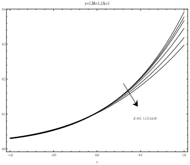
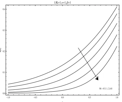
are plotted in the Figures1-4, respectively. Also Tables (1)-(4) show the obtained value ofu(0) for different values of parameters with two methods described in this manuscript. These tables show that our computations are more accurate.
Β =0.5, 1,1.5,3,6,10
-1.0 -0.5 0.0 0.5 1.0
0.0 0.1 0.2 0.3 0.4
x
u
@
x
D
Γ=1,M=1,1k=1
Figure 1: Variation ofβ onu
Γ = 0.5,1, 2,4,8
-1.0 -0.5 0.0 0.5 1.0
0.0 0.1 0.2 0.3 0.4 0.5
x
u
@
x
D
1K=1,M=1,Β=1
Figure 2: Variation ofγ onu
1/K = 0.5,1, 2,4,8
-1.0 -0.5 0.0 0.5 1.0
0.0 0.1 0.2 0.3 0.4
x
u
@
x
D
Γ=1,M=1,Β=1
Figure 3: Variation ofK onu
5
Numerical results
In this section, we have discussed the analytical and numerical results for Magnetohydrodynamic (MHD) Couette flow of third grade fluid between the two plates subject to nonlinear partial slip. The important finding in this paper is the com-bined effects of the nonlinear slip, MHD, porosity and the third grade fluid parameter on the ve-locity.Accurate numerical solutions are obtained using Ritz-Galerkin method in Bernstein polyno-mial basis.
Table 1: u(0) for γ= 1, M = 1 andβ = 1 for Ritz-Galerkin method (RGM) and Collocation method (CM)
withn= 7.
1/K RGM CM
0 0 0
0.5 0.0452078 0.0452073
1 0.029734126 0.029701378
2 0.0146237 0.0146159
4 0.00474728 0.00475515
8 0.000910552 0.000909626
Table 2: u(0) for γ= 1,M = 1 and 1
K = 1 for Ritz-Galerkin method (RGM) and Collocation method (CM)
withn= 7.
β RGM CM
0 0 0
0.5 0.0293163 0.02931436
1 0.029734126 0.029701378
1.5 0.03000307655120 0.02998722999818
3 0.0305548224868 0.0305542409344
6 0.0311526024483 0.031155063902
10 0.0315581316154 0.0315582
Table 3: u(0) forγ = 1, β = 1 and K1 = 1 for Ritz-Galerkin method (RGM) and Collocation method (CM)
withn= 7.
M RM CM
0 0 0
0.5 0.0435755 0.0435111
1 0.029734126 0.029701378
2 0.0154279 0.0153686
4 0.00528567 0.00527870
8 0.00106387 0.00106134
Table 4: u(0) for M = 1, β= 1 and K1 = 1 for Ritz-Galerkin method (RGM) and Collocation method (CM)
withn= 7.
γ RGM CM
0.5 0.0317452 0.0317472
1 0.029734126 0.029701378
2 0.0229654 0.0229626
4 0.015086 0.0151021
8 0.00883166 0.00883382
total adhesion to infinity. It is found that the ve-locity decreases by an increase inγ. The porosity analysis is carried out in Fig. 3. It is seen that with increase in porosity, velocity field decreases. Variation of MHD parameter is displayed in Fig. 2. This graph elucidate that the velocity decrease by increasing the MHD parameter.
The second set of results not only displays
solu-M = 0.5, 1, 2,4,8
-1.0 -0.5 0.0 0.5 1.0
0.0 0.1 0.2 0.3 0.4
x
u
@
x
D
1K=1,Γ=1,Β=1
Figure 4: Variation ofM onu
tions to the nonlinear problems arising in non-Newtonian fluid mechanics. As compared to other numerical techniques, such as finite differ-ences, the nonlinearity is not a major complica-tion for Ritz-Galerkin method in Bernstein poly-nomial method.
To the best of our knowledge, this is the first attempt to apply this robust and highly effective analytical technique as well as highly accurate method to study the non-Newtonian flows in this geometry. The results presented in this paper will now be available for experimental verification to give confidence for the well-posedness of this non-linear boundary value problem.
6
Conclusions
The properties of the Bernstein polynomials to-gether with the Ritz-Galerkin method are used to reduce the solution of the MHD Couette flow of non-Newtonian fluid in a porous medium to the solution of algebraic equations. The choice of ba-sis and ϕ(x) provides greater flexibility in which to impose boundary conditions. Numerical re-sults are included to demonstrate the validity and applicability of the new technique.
References
[1] C. Fetecau, C. Fetecau, Unsteady flows of Oldroyd-B fluids in a channel of rectangular
cross section, Int. J. Non-Linear Mech. 40
(2005) 1214-1219.
[2] C. Fetecau, C. Fetecau, Analytical solutions for non-Newtonian fluid flows in pipe like
domains, Int. J. Non-Linear Mech. 39 (2004)
225-231.
[3] W. C. Tan, T. Masuoka, Stokes’ first prob-lem for a second grade fluid in a porous
half space with heated boundary, Int. J.
Non-Linear Mech. 40 (2005) 512-522.
[4] W. C. Tan, T. Masuoka,Stokes’ first problem
for an Oldroyd-B fluid in a porous half space,
Phys. Fluids 17 (2005) 101-107.
[5] M. Hameed, S. Nadeem,Unsteady MHD flow
of a non-Newtonian fluid on a porous plate,
J. Math. Anal. Appl. 325 (2007) 724-733.
[6] M. Keimanesh, M. M. Rashidi, A. J. Chamkha, R. Jafari, Study of a third grade non-Newtonian fluid flow between two par-allel plates using the multi-step differential
transform method, Comput. Math. Appl. 62
(2011) 2871-2891.
[7] S. Abbasbandy, T. Hayat, F.M. Mahomed, R. Ellahi, On comparison of exact and se-ries solutions for thin film flow of a third
grade fluid, Int. J. Numer. Method Fluids
61 (2009) 987-994.
[8] R. Ellahi, P. D. Ariel, T. Hayat, S. Asghar,
Effect of heat transfer on a third grade fluid
in a flat Channel, Int. J. Numer. Methods
Fluids 63 (2010) 847-859.
[9] R. Ellahi, E. Shivanian, S. Abbasbandy, S.U. Rahman, T. Hayat, Analysis of steady flows in viscous fluid with heat transfer and slip
effects, Int. J. Heat Mass Transfer 55 (2012)
6384-6390.
[10] T. Hayat, R. Ellahi, F. M. Mahomed,
The Analytical solutions for Magnetohydro-dynamic flow of a of third order fluid in
a porous medium, Zeitschrift Fur
Natur-forschung A 64 (2009) 531-539.
[11] R. Ellahi, M. Hameed,Numerical analysis of steady non-Newtonian flows with heat
trans-fer analysis, MHD and nonlinear slip effects,
Int. J. Numer. Methods Heat and Fluid Flow 22 (2012) 24-38.
[12] K. R. Adeboye,H1-Galerkin-collocation and quasi-iterative method for boundary value
[13] M. Idrees Bhatti, P. Bracken, Solutions of differential equations in a Bernstein
poly-nomial basis, J. Comput. Appl. Math. 205
(2007) 272-280.
Zahra Barikbin is an Assistant pro-fessor in the department of math-ematics, Imam Khomeini Interna-tional University, Ghazvin. She was graduated in Shahid Beheshti University of Tehran and her main research interests include numeri-cal solution of Partial Differential Equations, In-tegral Equations and computational mathemat-ics.
Ramat Ellahi is founder Chairper-son of the Department of Mathe-matics and Statistics at IIUI, Pak-istan. He has several awards and honors on his credit: Fulbright Fel-low University of California USA, Productive Scientist of Pakistan, Best University Teacher Award by higher edu-cation commission (HEC) Pakistan, Best Book Award, and Valued Reviewer Award by Elsevier. He is also an author of six books and editor of five international journals.