Biogeosciences, 6, 807–817, 2009 www.biogeosciences.net/6/807/2009/
© Author(s) 2009. This work is distributed under the Creative Commons Attribution 3.0 License.
Biogeosciences
Comparing high resolution WRF-VPRM simulations and two global
CO
2
transport models with coastal tower measurements of CO
2
R. Ahmadov1, C. Gerbig1, R. Kretschmer1, S. K¨orner1, C. R¨odenbeck1, P. Bousquet2, and M. Ramonet2 1Max-Planck-Institute for Biogeochemistry, Hans-Kn¨oll-Str. 10, 07745, Jena, Germany
2Laboratoire des Sciences du Climat et de l-Environnement, UMR CEA-CNRS 1572, 91191 Gif-sur-Yvette, France
Received: 29 September 2008 – Published in Biogeosciences Discuss.: 5 December 2008 Revised: 20 April 2009 – Accepted: 4 May 2009 – Published: 15 May 2009
Abstract. In order to better understand the effects that mesoscale transport has on atmospheric CO2 distributions,
we have used the atmospheric WRF model coupled to the diagnostic biospheric model VPRM, which provides high resolution biospheric CO2 fluxes based on MODIS
satel-lite indices. We have run WRF-VPRM for the period from 16 May to 15 June in 2005 covering the intensive period of the CERES experiment, using the CO2 fields from the
global model LMDZ for initialization and lateral boundary conditions. The comparison of modeled CO2concentration
time series against observations at the Biscarosse tower and against output from two global models – LMDZ and TM3 – clearly reveals that WRF-VPRM can capture the measured CO2 signal much better than the global models with lower
resolution. Also the diurnal variability of the atmospheric CO2field caused by recirculation of nighttime respired CO2
is simulated by WRF-VRPM reasonably well. Analysis of the nighttime data indicates that with high resolution mod-eling tools such as WRF-VPRM a large fraction of the time periods that are impossible to utilize in global models, can be used quantitatively and may help to constrain respiratory fluxes. The paper concludes that we need to utilize a high-resolution model such as WRF-VPRM to use continental ob-servations of CO2concentration data with more spatial and
temporal coverage and to link them to the global inversion models.
Correspondence to: R. Ahmadov
1 Introduction
There is clear evidence in climate science that the contin-ued increase of the atmospheric CO2 content is caused by
the anthropogenic emissions. However one of the scien-tific challenges is understanding the mechanisms responsible for removing anthropogenic CO2from the atmosphere.
Ob-servations demonstrate that about half of the emitted CO2
is absorbed by biospheric sinks – the terrestrial biosphere and the ocean (Hansen et al., 2007). There are a number of essential questions related to the biogeochemical cycle of CO2 to be solved by the scientific community. Modern
coupled atmosphere-biosphere models suggest that, terres-trial ecosystems will provide a positive feedback in a warm-ing world on a global scale (Heimann and Reichstein, 2008), which makes it essential to study the role and evolution of the giant natural carbon reservoirs. The leading questions are first of all the determination and also estimation of pro-cesses by which anthropogenic CO2is sequestered in the
na-ture. It is also crucial to know the feedback mechanisms be-tween the natural carbon cycle and the global climate system. The attempt to mitigate and also control the greenhouse gas emissions from different regions and countries requires esti-mating their carbon budget, which is a big challenge in the atmospheric sciences.
In order to answer the above mentioned questions, the at-mospheric measurements of CO2from global networks are
used in combination with inverse analysis to retrieve infor-mation on biosphere-atmosphere fluxes (Tans et al., 1990; Gurney et al., 2002). These approaches were operated based on annual and monthly atmospheric observations. Conse-quently the flux estimations of such inversion studies were very coarse in both time and space.
continental sites were surface stations located on mountains and near coasts. In order to increase the representativeness of measurements sites, tall towers equipped with meteorolog-ical and greenhouse gas measurement devices were imple-mented to carry out CO2measurements at about 300 m above
ground (Bakwin et al., 1995). Nevertheless, the location of any continental measurement site close to variable sources is often located in meteorologically complex areas: terrain-induced mesoscale phenomena such as sea-land (lake, river, forest, etc.) breezes, mountain-valley circulations, urban heat islands etc. make their representation in atmospheric models quite difficult.
Mesoscale effects generated by land surface heterogene-ity and complex topography are usually on subgrid scales of current generation transport models used in inversions. In ad-dition high resolution models are able to capture more accu-rately the front passing time and related effects at a site. An accurate simulation of front passing time at a measurement station is crucial since this may lead to strong jumps in CO2
concentration (Wang et al., 2007). Further, in a model with coarse resolution complex boundary layer structures and thus vertical profiles of CO2 over heterogeneous land cannot be
adequately resolved. Mesoscale flows and mixing in the at-mosphere are strongly correlated with short term variability of biospheric CO2fluxes, since they are both driven by the
same mechanism, solar radiation. Hence inappropriate rep-resentation of the atmospheric transport on mesoscales may lead to significant biases in biospheric sources and sinks de-rived from inverse modeling. Thus all these effects can only be addressed with high resolution mesoscale simulations that include CO2fields in order to bridge the gap between
mea-surements and inversion models.
The strong deterioration of CO2inversions due to transport
model deficiencies are proven in some studies (Lin and Ger-big, 2005; Gerbig et al., 2008). In these studies uncertainties in advection and vertical mixing from ECMWF and ETA me-teorological models are quantified and then linked to result-ing errors in CO2inversions. The transport deficiencies
be-come especially critical when trying to invert high space/time resolution of fluxes as compared to monthly fluxes on large regions for which data limitation is probably larger (Gur-ney et al., 2002). A comprehensive validation of differ-ent global (TM3, LMDZ) and regional (HANK, DEHM, REMO) offline transport models were done by (Geels et al., 2007) for several European tall towers and mountain stations. The intercomparison study revealed the remarkable improve-ment of the CO2concentration simulation by regional
mod-els with horizontal resolutions down to 50 km compared to the coarser global models. The conclusions made by Geels et al. (2007) impose severe limitations on the usability of continental CO2 concentration data from short towers and
mountain stations in inversions. Moreover one may also add coastal stations to the “difficult sites” list (Riley et al., 2005). As a result, the CO2 inversions performed by the
TransCom 3 inversion community down-weighted
continen-tal observations, assuming that the data contained too much “noise” (Gurney et al., 2004; Wang et al., 2007).
Another problem is the requirement of strict temporal data selection in inversions. Global CO2 inversions usually use
only afternoon hourly or even averaged values. Nighttime data or measurements taken during morning and evening hours are not used for most of the continental sites. Some of the inversion studies involve further filtering for day to day variability of CO2 observation data to remove the “noise”.
Such filtering leads to losing the information about diurnal cycle of biospheric signals, which contains information on biospheric processes – respiration and photosynthesis, where for instance using nighttime data would make possible to constrain respiration fluxes. Thus it would be an obvious gain to use the full time series of continuous data for the inversion rather than only afternoon values. Using high-frequency con-centration data would also be very useful for regional scale inversions which also could assist to close the gap between top-down and bottom-up estimations (Law et al., 2002).
As pointed out by Gerbig et al. (2009) there are several ways to mitigate the shortcomings of current inversion sys-tems associated with uncertainties in transport representa-tion of meteorological fields used for global inversion mod-els. One of the promising solutions would be to apply trans-port models which better reproduce these processes. There are few studies addressing this problem by involving high-resolution atmosphere-biosphere models. Several mesoscale modeling systems are currently used to simulate mesoscale variations of CO2concentration in the atmosphere (e.g.
Den-ning et al., 2003; van der Molen and Dolman, 2007; Sar-rat et al., 2007; Ahmadov et al., 2007). In these studies mesoscale meteorological models in combination with bio-spheric models were used to perform forward simulations of CO2. The studies show how strongly mesoscale flows
initi-ated by complex terrain and by the land-water contrast could lead to remarkable gradients in atmospheric CO2fields. Such
mesoscale model validations are also valuable since their me-teorological fields can be used in regional inversions (Lau-vaux et al., 2008).
This paper discusses the advantages of using very high-resolution mesoscale simulations for CO2 transport versus
two global CO2transport models in case of a coastal
concen-tration measurement station – Biscarosse tower. The main goal of the paper is to address the deficiencies of the coarse resolution transport models in representing CO2point
mea-surements which we have to take into account in the inver-sions targeted to estimate CO2fluxes. In addition the paper
R. Ahmadov et al.: WRF-VPRM simulations of CO2 809
Longitude
Latitude
Terrain height, m
−2 −1.5 −1 −0.5 0 0.5 1 1.5
43.5 44 44.5
45 45.5
0 500 1000 1500 2000
Longitude
Latitude
Terrain height, m
−4 −3 −2 −1 0 1 2 3 4
42 43 44 45 46 47 Figure 1
a) b)
Fig. 1. Topography of the WRF domains – (a) the outer grid with 10 km resolution, the white box depicts boundaries of the inner domain, and (b) the inner grid with 2 km resolution, the white triangle indicates the Biscarosse tower location.
In Sect. 2 we describe the model setup. Section 3 intro-duces the observation campaign and the measurements. Sec-tion 4 presents a comparison of WRF-VPRM modeling re-sults, global models and the observations. Finally, Sect. 5 summarizes the paper and discusses advantages and perspec-tives of using the WRF-VPRM modeling system for assimi-lating CO2concentration data from continental sites.
2 Configuration of the models
We set up and ran the Weather Research and Forecasting (WRF) model (http://wrf-model.org) at 10 and 2 km reso-lution on two nested grids (see Fig. 1a, b) over a domain that encompasses the area of the measurement campaign de-scribed in Sect. 3. The model was run in the two-way nested mode. In the two-way nest integration, the outer domain with 10 km (Fig. 1a) resolution provides the inner one (Fig. 1b) with lateral boundary conditions for the meteorological and CO2 fields at every time step, simultaneously the 2 km grid
solution replaces the 10 km grid solution for the points that lie inside the inner domain.
We coupled the diagnostic biospheric model Vegetation Photosynthesis and Respiration Model (VPRM) (Mahadevan et al., 2008) to WRF as a module. A detailed description of the WRF-VPRM modeling system can be found in (Ah-madov et al., 2007), here we provide only a brief overview. The VPRM model produces biospheric CO2fluxes in order
to perform CO2 tracer transport by WRF. The model uses
MODIS (http://modis.gsfc.nasa.gov) satellite indices – en-hanced vegetation index (EVI) and land surface water index (LSWI) obtained in 500 m spatial resolution with 8 days fre-quency. VPRM uses eight land-use classes with different parameters constraining CO2 uptake and respiration fluxes.
These parameters were optimized by using CO2 flux
mea-surements at few land-use classes located in the modeling
domain. Furthermore the model used air temperature and ra-diation fields from the WRF model. For the VPRM model a high-resolution land cover map – SYNMAP (Jung et al., 2006) was used. A special preprocessing tool was used to preprocess land-use data and MODIS indices to map on a WRF grid. The preprocessing tool and the WRF-VPRM code are available freely to users upon request.
Anthropogenic CO2 fluxes were taken from the 10 km
resolution European anthropogenic emission inventory (up-dated in October, 2005) developed by the Institute of Eco-nomics and the Rational Use of Energy (IER), University of Stuttgart (http://carboeurope.ier.uni-stuttgart.de/). Lateral boundary conditions (LBCs) and initial conditions (ICs) for CO2concentration fields were taken from the global zoomed
CO2 transport model – LMDZ (Hourdin and Armengaud,
1999; Peylin et al., 2005) with a horizontal resolution of 0.83◦×1.25◦ (latitude×longitude) over Europe, 28 vertical levels up to the tropopause, and half hourly time resolution (hourly for outputs) for physical processes (3 min for dy-namical processes). The model is nudged to the ECMWF (http://www.ecmwf.int/) global model data to perform the meteorological transport. The LMDZ CO2fields used here
are based on forward runs using CO2fluxes generated by the
ecophysiological model – SiB2 (Sellers et al., 1996) together with fossil and ocean fluxes. Further an offset (376 ppm) was added to the model output to fit some of the European mea-surement sites.
All necessary meteorological data for initial and lateral boundary conditions, sea surface temperature and soil initial-ization fields of WRF were taken from the ECMWF analysis data (http://www.ecmwf.int/) with≈35 km horizontal reso-lution and 6 hourly intervals.
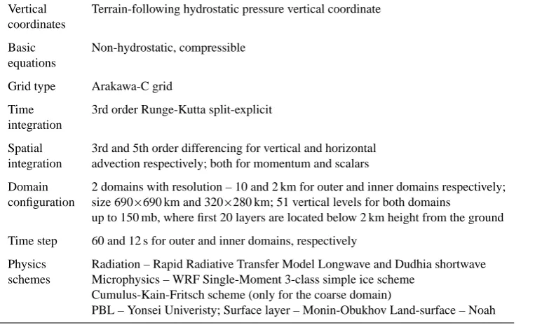
Table 1. Parameters and physics options used in the WRF model.
Vertical Terrain-following hydrostatic pressure vertical coordinate coordinates
Basic Non-hydrostatic, compressible equations
Grid type Arakawa-C grid
Time 3rd order Runge-Kutta split-explicit integration
Spatial 3rd and 5th order differencing for vertical and horizontal integration advection respectively; both for momentum and scalars
Domain 2 domains with resolution – 10 and 2 km for outer and inner domains respectively; configuration size 690×690 km and 320×280 km; 51 vertical levels for both domains
up to 150 mb, where first 20 layers are located below 2 km height from the ground
Time step 60 and 12 s for outer and inner domains, respectively
Physics Radiation – Rapid Radiative Transfer Model Longwave and Dudhia shortwave schemes Microphysics – WRF Single-Moment 3-class simple ice scheme
Cumulus-Kain-Fritsch scheme (only for the coarse domain)
PBL – Yonsei Univeristy; Surface layer – Monin-Obukhov Land-surface – Noah
Macatangay et al., 2008). One improvement of WRF-VPRM in the current study is the online coupling of VPRM to WRF, so that WRF produced air temperature at 2 m (T2) and short-wave downward radiation (SWDOWN) were used in VPRM to calculate CO2 fluxes which were then provided to WRF
at each integration time step. Table 1 shows the WRF model physics and grid options for these runs. In WRF-VPRM we used several concentration fields, so called “tagged tracers”, for CO2corresponding to the different origins: 1) total CO2
concentration (which can be measured) that combines CO2
fields from anthropogenic and biospheric sources and also coming from the outside of the simulation domain; 2) global CO2 that does not include any uptake or emission fluxes
within the WRF domains, which participates only in trans-port; 3) anthropogenic CO2; 4) respiration and 5)
photosyn-thesis signals. The last three “tagged” tracers include only the corresponding surface fluxes. They use zero inflow and zero-gradient outflow lateral boundary conditions, zero fields for initial conditions. The first two “tagged” tracers use CO2
concentration fields from a global model in inflow and zero-gradient conditions on outflow, global fields for ICs. The “tagged” tracers allow us to separate the global CO2signal
from the regional one, and to determine the contribution of the different fluxes to the total CO2signal.
All anthropogenic and biospheric fluxes were added at each simulation time step to the CO2field in the lowest
ver-tical level of the WRF grids. We ran WRF-VPRM for one month time period – from 16 May to 15 June, 2005. Here only simulation results from the high-resolution (2 km) inner nest are presented.
Another model involved in this study is the TM3 global model (R¨odenbeck et al., 2003) with a horizontal resolution of 4◦×5◦ (latitude×longitude), 19 vertical levels up to the
tropopause, and hourly time resolution (using instantaneous concentrations every 3 h for output). It uses 6-hourly NCEP data as meteorological input. The purpose of adding this model to the comparison is to get an insight into how increas-ing resolution improves the simulation of CO2 variability.
The TM3 model results are based on a global inversion us-ing atmospheric CO2concentration measurements.
BIOME-BGC (Trusilova and Churkina, 2008) was used to generate CO2fluxes from the terrestrial biosphere as a prior for the
TM3 inversion. It should be noted that the TM3 model did not use the Biscarosse site in the optimization of the surface fluxes.
3 CERES campaign
R. Ahmadov et al.: WRF-VPRM simulations of CO2 811
(Bordeaux) edges of the domain. According to the local cli-matology the dominant winds should be either from the west or the east; therefore, the experiment was designed to ob-serve modification of the CO2concentration profiles by the
land as the air mass progressed east- or westward (Dolman et al., 2006).
During the campaign CO2 concentration measurements
were carried out by several surface stations and also by air-craft (Ahmadov et al., 2007). Several CO2eddy-flux and
sur-face meteorological stations were also deployed during the experimental campaign. A high-precision CO2 instrument
(CARIBOU, with an accuracy of 0.1 ppm) was installed and operated on a 40-m high tower near Biscarosse (44.38◦N, 1.23◦W) (Fig. 1b) (Dolman et al., 2006). The measurement site is located about 2 km from the sea shore, and about 120 m above sea level. In addition we involved data from the mete-orological station BISCAROSSE/PARENTIS located in the vicinity (44.43◦N, 1.25◦W) of the tower to aid interpreting CO2measurements, given that there were no meteorological
measurements made at the tower itself. During the campaign other surface CO2stations (e.g. in Marmande and La Cape
Sud areas) were operated, however those measurements were taken very close to the ground. Therefore we have involved only the Biscarosse site in this study.
The Biscarosse site is located at 2 km distance from the coast (Fig. 1b), thus the small area of the land biosphere be-tween the tower and the ocean is not expected to change the marine air masses’ CO2content significantly while the air is
transported to the site by westerlies. Thus the tower detects marine air masses, with measurement periods that have large scale representativeness, but also air masses coming from in-land with influences from the terrestrial biosphere and an-thropogenic emissions. We chose this site for the current study assuming that the Biscarosse data might be used in fu-ture inversion studies (Lauvaux et al., 2008).
4 Results and discussion
Here we present the results for WRF-VPRM simulations for the Biscarosse site and the nearby weather station. Figure 2 exhibits a comparison of air temperature (T2) simulated by WRF and observed by the meteorological station. This plot gives insight into weather evolution over the period as well as the model performance for the important meteorologi-cal variable (T2), which also drives biospheric CO2 fluxes.
After a cold front passed on 17 May the weather became warmer, with sunny conditions on the following days. The south-westerly flows were bringing warm air masses to the region and thereby keeping the air temperature very high dur-ing 25–27 May. The fair weather was followed by synoptic perturbations and colder temperatures next days, except 1–2 June. On 8 June again anticyclonic conditions started pre-vailing and persisted until 12 June. Later the weather became cloudy and rainy over France by westerly flows pushed by
21−May 26−May 31−May 05−Jun 10−Jun 15−Jun 5
10 15 20 25 30 35
Tair, C
°
Tair, model Tair, observation Figure 2
Fig. 2. Comparison of air temperature at 2 m between WRF sim-ulated and measured one at the meteorological station – Biscar-rosse Parentis. The statistics: r2=0.77, average bias is−0.74◦C, RMSE=2.14◦C.
a cyclone. The comparison reveals that the high-resolution model is able to accurately predict temperature variations with only a slight cold bias.
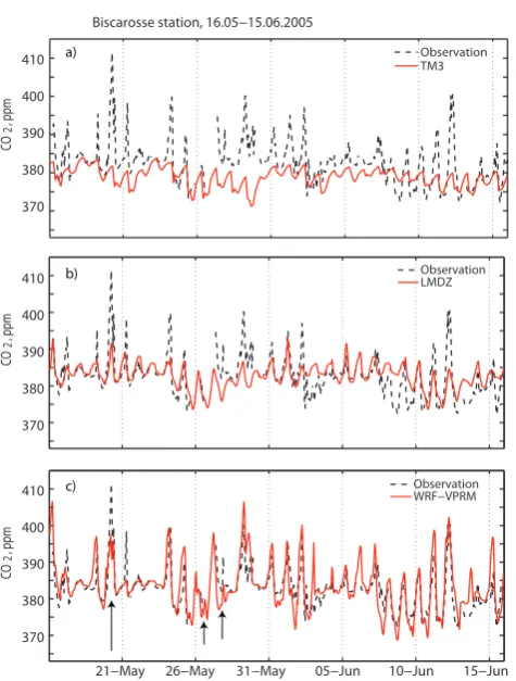
Figure 3a, b and c shows hourly CO2concentration
mea-surements at the Biscarosse tower during one month to-gether with simulated CO2from the global models TM3 and
LMDZ, and from the mesoscale model WRF-VPRM. The figure shows how the models perform in capturing day to day variability of the concentration. Figure 3c shows that the WRF-VPRM model can capture much more variability in the observed time series than the two global models. Also the signal’s amplitude of the signal is captured reasonably well for both daytime minimum and nighttime maximum by WRF-VPRM in many cases. Unlike the global mod-els, WRF-VPRM is able to simulate the second maximum of CO2concentration in daytime which appeared due to the
front passage or sea breeze in some days, e.g. during the 20, 26 and 27 May (Fig. 2).
The TM3 model shows some bias and less correlation with the observed data compared to LMDZ, which is as we argue due to its coarser resolution. For example, due to the gridcell size of several hundred kilometers within TM3 it is impossi-ble to represent a coastal station correctly by the model under all flow conditions. The grid box comprising the Biscarosse tower is fully located over land in TM3, therefore the land influence is significantly overestimated, leading to stronger uptake as compared to the observations. It is worthy to note that TM3 and LMDZ have comparable performances when used with comparable resolution (Law et al., 2008).
LMDZ captures the observed daytime minimum and nighttime maximum in CO2 concentrations with some
Table 2. Statistics of the comparison between measured and simulated CO2from the models for different cases – hourly, afternoon and nighttime averaged;R2– the square of the correlation coefficient, Bias- the mean bias, RMSE – root mean square error is the standard deviation of the differences between the models and the observations; Mean(stdobs)– the averaged standard deviation of the high-frequency CO2measurements from their hourly means.
Time Model R2 Bias, ppm RMSE, ppm Mean(stdobs), ppm
Hourly
TM3 0.16 −3.87 5.09
0.58
LMDZ 0.29 0.11 4.66
WRF-VPRM 0.59 0.67 4.26
Afternoon Averaged
TM3 0.06 −2.49 3.67
0.35
LMDZ 0.18 0.95 3.28
WRF-VPRM 0.52 −0.27 3.42
Nighttime Averaged
TM3 0.02 −6.76 6.68
1.05
LMDZ 0.22 −1.91 6.1
WRF-VPRM 0.58 0.95 4.95
Biscarosse station, 16.05−15.06.2005
CO
2
, ppm
Observation TM3
370 380 390 400
410 ObservationLMDZ
21−May 26−May 31−May 05−Jun 10−Jun 15−Jun 370
380 390 400
410 ObservationWRF−VPRM
370 380 390 400 410
CO
2
, ppm
CO
2
[image:6.595.50.288.321.635.2], ppm
Figure 3
a)
b)
c)
Fig. 3. CO2 concentration time series from the Biscarosse tower and the models – (a) TM3, (b) LMDZ, (c) WRF-VPRM, the black arrows point different days: 20, 26 and 27 May.
resolution, it cannot accurately resolve subdiurnal variability in CO2concentration associated with atmospheric transport
and mixing processes near the coastline.
The relevant statistics for the model-data comparisons can be found in Table 2, where also the mean standard devi-ation within the measurement periods of one hour is pre-sented. The high root mean square error (RMSE) in the model-measurement comparison is partially caused by aver-aging the measurements over each hour, while using instan-taneous values in the models. Averaging in the observation data is necessary to minimize the effects of eddies and other small scale effects that are not resolved by any of the mod-els. Interestingly, the variability of CO2within an hour (last
column of Table 2) is a factor of three smaller during day than during night, most probably due to stronger and deeper vertical mixing.
The numbers in Table 2 show that WRF-VPRM exhibits much more correlation compared to the global models. The main reason for such agreement is a better representation of the transport, especially mesoscale flows and vertical mix-ing in the 2 km resolution WRF-VPRM runs. In addition, the more accurate representation of the fine-scale variability in the surface CO2fluxes by VPRM, especially in the site’s
near-field, improves the CO2simulation as compared to the
coarser global models. Although the average bias in LMDZ against hourly observation data is smaller, its deviation from the measurements (RMSE) is greater than in WRF. The ex-isting discrepancy between the WRF-VPRM model and the measurements is caused by several reasons – uncertainties in CO2fluxes simulated by VPRM, initial and boundary
condi-tions of CO2from LMDZ model, also uncertainties in
R. Ahmadov et al.: WRF-VPRM simulations of CO2 813
et al., 2008). Yet, the quality of VPRM fluxes would un-doubtedly benefit from an optimization against atmospheric concentration measurements, while we only optimized the VPRM parameters against flux data from a few sites oper-ated during the campaign (Ahmadov et al., 2007). VPRM is able to mimic the spatial and temporal distribution of sur-face fluxes by using high resolution satellite indices, land-use map and high spatiotemporal resolution meteorological fields from WRF. This approach is sufficient to determine the influence of main transport and mixing capabilities of the model on the CO2distribution.
In order to make clearer the contribution of different sources to the CO2concentration at the measurement
loca-tion, we present hourly time series of the different “tagged” tracers from the WRF-VPRM model (Fig. 4). There is release of CO2 by biosphere and accumulation of
anthro-pogenic CO2in the shallow nighttime boundary layer.
Dur-ing some nights, for instance on 20 May there is an evident enhancement of both the biospheric and anthropogenic CO2
fields since the tower detects inland respired CO2and also
emission from power plants and other anthropogenic sources, but respired CO2largely dominates in amplitude. The
ana-lyzed time series reveal that in the CERES region during the summer season the biospheric CO2fluxes are dominant
com-pared to the anthropogenic emissions, therefore we may ne-glect the anthropogenic component in further interpretations of the observations.
During persistent strong westerly winds (e.g. 21–23 May, 2005) both the biospheric and the anthropogenic CO2
con-centration at the site become negligible. In such instances the global CO2tracer plays the main role in contributing to the
measured signal. During June the overall CO2uptake signals
are stronger than during May, the first part of the simulation period. This behavior is caused by phenological changes as-sociated with the intensifying growing season. Some of the large cropland areas in the region become strong CO2sinks
in June as shown by Ahmadov et al. (2007).
A recirculation of respired nighttime CO2fields, for which
the term “3-D rectifier effect” was established (Riley et al., 2005; P´erez-Landa et al., 2007; Ahmadov et al., 2007) is demonstrated for the case 20 May, 2005 (Fig. 5). During this day a south-westerly flow brought warm air masses over France. The weather was warm (Fig. 2) and sunny, with only some high clouds and weak westerly winds observed near the surface. It is obvious that this condition favors the formation of sea-land breeze, which enhances the westerly wind component of the surface wind towards afternoon. It is noteworthy that during this night the highest CO2signal
of the May–June period at the Biscarosse tower was regis-tered, with an enhancement of about 30 ppm compared to the afternoon values (Fig. 3a).
As Fig. 5a shows, WRF-VPRM underestimates this signal by about 10 ppm during the early morning when the noctur-nal boundary layer is enriched with respired CO2advected
from the inland by weak easterly winds (Fig. 5b). The
un-21−May 26−May 31−May 05−Jun 10−Jun 15−Jun 360
370 380 390 400 410
CO
2
, ppm
Biscarosse tower, 16 May − 15 June, 2005
observation Biospheric+376 Anthropogenic+376 Global
Total−model Figure 4
Fig. 4. Time series of the different tagged tracers at the tower site from the WRF-VPRM model.
derestimation might be related to overestimation of the east-erly wind in WRF during that night when comparing to the measurements at the nearby weather station (Fig. 5c). There was stagnation in the air in early morning caused by conver-gence of westerly wind and land breeze. During this time the tower detected only respired CO2 from the ground
be-neath. Since WRF could not well capture this case occurring around 05:00 UTC (07:00 local time), it failed also to resolve the huge respired CO2 concentration by that time (see the
“respired CO2” tagged tracer time series in Fig. 5a). It is
in-teresting to see that WRF-VPRM captures the minimum in CO2concentration at around 08:00 UTC (although 2 h
ear-lier), associated with the change in wind through southerly at the onset of the sea breeze (Fig. 5b). Close to 10:00 UTC the strengthening and reversing wind flow becomes more west-erly and brings a large plume of CO2 respired during the
previous night. Therefore we see a second strong maximum near 10:00 UTC in the measurement, but again a bit earlier in WRF-VPRM (Fig. 5a), since the wind rotation is faster in the model. After a few hours the westerly winds start bringing marine air masses with lower constant CO2concentration
un-til the next day. The model captured this very well, indicating that the lateral boundary condition from the LMDZ model is appropriate. TM3 and LMDZ both show a smoothed diurnal cycle of CO2without a second maximum during this day due
to coarse resolution.
In cases of strong synoptic disturbance the diurnal CO2
signal at the site looks very different. For instance, on the 18 May, 2005 after the crossing of a cold front during the previous day, the wind shifted to north-west over the western part of France, colder and drier air moved into the country (Fig. 2). During this day the diurnal CO2concentration
vari-ation measured at the Biscarosse tower was less than 5 ppm (Fig. 3a). These are ocean air masses which are not affected by diurnal CO2fluxes as on the continent. This case was well
CO
2
, ppm
0 5 10 15 20
0 2 4 6 8 10
wind speed, m/s
0 5 10 15 20
0 100 200 300
wind direction, degrees
WRF obs.
a) b)
c)
0 5 10 15 20
370 380 390 400 410
hour
Biscarosse station, May-20, 2005
WRF-VPRM LMDZ Observation TM3 Respired + 376
Fig. 5. (a) CO2concentrations from the models versus the observation for the 20 May, and respired tagged CO2tracer from WRF-VPRM; (b) wind direction and (c) wind speed comparison on that day at the nearby meteorological station; the time is given in UTC.
Biscarosse station, 16.05−15.06, 2005 WRF−VPRM LMDZ TM3 Observation
21−May 26−May 31−May 05−Jun 10−Jun 15−Jun
370 375 380 385 390 395 400 405
CO
2
, ppm
21−May 26−May 31−May 05−Jun 10−Jun 15−Jun
370 375 380 385 390 395 400 405
CO
2
, ppm
Figure 6
a) b)
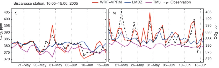
Fig. 6. Comparison of measured CO2concentration against the models for (a) daytime and (b) nighttime averaged cases.
Since in the global inversions usually afternoon CO2
con-centration data is used it is important to check how realis-tically the models used here simulate this kind of data. We analyzed CO2 concentration time series averaged for
day-time between 12:00 UTC to 17:00 UTC, which characterize the well-mixed hours for the region. Figure 6a demonstrates a comparison between all the models and the observation for the averaged concentration time during the well-mixed hours within one month period. The related statistics for the com-parison are given in Table 2, indicating increasing correla-tion with increasing horizontal resolucorrela-tion. According to Ta-ble 2, the LMDZ model generally represents day-to-day vari-ability of the afternoon averaged concentrations, while TM3 shows lower performance, especially in magnitude due to the above mentioned negative bias. The mean bias in LMDZ is larger than in WRF-VPRM. Only the root mean square errors are high in both models and even slightly bigger in WRF-VPRM. This can be explained by larger variability in the high-resolution model which leads to more scattering of the model predicted CO2fields (Fig. 3c). WRF-VPRM and
LMDZ show quite good agreement against the observation
until 27 May. On the following days we see a remarkable mismatch in the global models. On 30 May the observa-tion showed the highest CO2signal during this period. Both
LMDZ and TM3 underestimate this signal. However, WRF-VPRM captures this highest signal with some overestima-tion.
Focusing on night-time concentration (05:00–07:00 UTC, representing the later part of the night), WRF-VPRM agrees much better with the observations as compared to global models (Fig. 6b). From Fig. 6b and Table 2 it can be seen that generally the correlation between the models and the obser-vation is slightly higher during night than during day; usu-ally all models predict an early morning maximum in CO2
concentrations due to release of CO2into nocturnal
bound-ary layers. But the global models show significant deviation from the observation for the nighttime data. This discrep-ancy is caused by a poor simulation of nighttime vertical mixing. The correlation coefficients for both daytime and nighttime averaged CO2concentrations are significantly
[image:8.595.87.510.292.424.2]R. Ahmadov et al.: WRF-VPRM simulations of CO2 815
well, while there is some bias in amplitude, but much smaller than in the global models. This fact indicates that also for a mesoscale model such as WRF it is difficult to parameterize the nocturnal stable boundary layer, which is an active area of research in meteorology (Steeneveld, 2007).
5 Conclusions
We have used the high-resolution coupled atmosphere-biosphere model WRF-VPRM in order to interpret CO2
con-centration time series observed from a tower at the coastal station near Biscarosse during the CERES campaign in 2005. The station is strongly influenced by mesoscale flows. Sea-land breeze and its combination with local CO2 fluxes can
lead to a significant “contamination” of the observation sig-nal, such that the time series is problematic to use quanti-tatively in coarse models. These errors come also from the poor simulation of vertical mixing during night and day over land. Similarly these kinds of errors are typical for stations located on complex terrain such as mountains.
Simulated CO2from two global models used in CO2
in-versions, TM3 and LMDZ, with different spatial resolutions, were compared with tower observations as well as with high-resolution simulation results from the coupled atmosphere-biosphere model WRF-VPRM. The results have shown that only WRF-VPRM is able to simulate the observed diurnal variability. The simulations also confirmed that recircula-tion of nighttime respired CO2requires modeling the
covari-ance of mesoscale circulation and biospheric fluxes. Thus when our models are not able to simulate nighttime CO2,
then this may imply the “repeated bias” in daytime simula-tions due to recirculation with sea-breeze effect or in some cases frontal passage. One may conclude from such situ-ations that even averaging CO2 measurements over periods
with a well-mixed boundary layer cannot prevent a contami-nation from recirculated continental respiration signals; con-sequently large representation errors in inversions when us-ing such data are expected.
The work clearly demonstrates that an appropriate repre-sentation of synoptic variations and mesoscale effects can substantially improve representation of hourly CO2.
Un-doubtedly a part of the differences between the models are caused by differences in the parameterizations, especially within the PBL schemes. WRF can be run with a different choice of PBL schemes, which in future studies should be used to investigate their impact and to validate these schemes using WRF-VPRM in comparison to CO2observations as a
passive tracer.
Although we used fluxes from the simple diagnostic VPRM model that were not optimized against concentration measurements, the WRF-VPRM model is able to capture much more variability in the tower measured CO2time
se-ries. This indicates the importance of capturing the transport and mixing processes at high resolution and the
spatiotempo-ral variability of biospheric fluxes that VPRM can represent. The high-resolution representation of the spatial heterogene-ity in CO2fluxes especially in the near field is very
impor-tant for properly simulating CO2distribution (Gerbig et al.,
2009). In addition, a proper representation of the covariance between meteorology and biospheric CO2flux is necessary
to capture rectifier effects (both, the normal rectification ef-fect as well as the 3-D rectification efef-fect) in order to avoid bias errors (Ahmadov et al., 2007).
This paper shows the potential of using WRF-VPRM in the context of inverse modeling in order to utilize high-frequency CO2concentration data. This is likely to improve
inversion accuracy, and could extend the inverse modeling to “difficult sites” not used in current inversions. Running WRF-VPRM in very high resolution at global scale is com-putationally expensive, and needs to be used efficiently to-gether with global inversion models. The run time of WRF-VPRM for one day on the 2 km grid is about 2–3 h on an Opteron cluster using 8 nodes (4 processors per node).
It is feasible to setup small domains around some measure-ment stations and to run a mesoscale model such as WRF-VPRM for these domains in high spatial resolution depend-ing on the region and topography. Regional scale inversions can be done using the STILT-VPRM modeling framework (Matross et al., 2006), which can be driven by WRF gener-ated transport fields. R¨odenbeck et al. (2009) showed that such nested inversions within global models are feasible, even with completely different transport representations for global and regional scales. Moreover forward modeling of CO2transport by WRF-VPRM for some sites is an essential
to validate the model, and provides a better understanding of near-field influence on measurements at continental sites and consequently on regional flux estimates (Lauvaux et al., 2008). Using such flexible modeling tools as WRF would al-low us to test different physics and dynamics options in order to improve modeling capabilities for a given region.
The agreement of nighttime simulated CO2 with
obser-vations suggests that it should be feasible to also use the nighttime observations in the inversions, providing impor-tant information on the partitioning of biosphere-atmosphere exchange between respiration and photosynthesis. Lauvaux et al. (2008) has found that improving the transport simula-tion for nocturnal CO2 concentrations at tower sites would
lead to large error reduction in CO2 inversions. Although
proper simulation of the stable boundary layers remains diffi-cult even in advanced mesoscale models such as WRF, there is hope that within the large community involved in WRF model development (http://wrf-model.org) there will be sub-stantially improvements in its capabilities to simulate mixing in nighttime cases. Inversion studies would be able to con-strain respiration fluxes at regional scales using the numerous continuous CO2monitoring sites by involving nighttime data
Because of its great flexibility, WRF-VPRM can serve to bridge the gap between the measurements and inversion models in almost all regions of the globe including complex terrain areas. The fast growing global greenhouse gas moni-toring network makes this tool attractive.
Acknowledgements. The authors are grateful to all the CERES
community for providing the measurement results. We thank the technical teams from RAMCES and DAPNIA/SIS for the mainte-nance of the CARIBOU analyzer. We acknowledge G. Boenisch from MPI BGC for the help in getting the meteorological data from the NOAA database. We thank S. Schott for her support in the layout. The authors appreciate the valuable comments of the two reviewers R. Law and A. Meesters.
Edited by: H. Dolman
The service charges for this open access publication have been covered by the Max Planck Society.
References
Ahmadov, R., Gerbig, C., Kretschmer, R., et al.: Mesoscale covari-ance of transport and CO2fluxes: Evidence from observations and simulations using the WRF-VPRM coupled atmosphere-biosphere model, J. Geophys. Res.-Atmos., 112(D22), D22107, doi:10.1029/2007JD008552, 2007.
Bakwin, P. S., Tans, P. P., Zhao, C. L., Ussler III, W., and Quesnell, E.: Measurements of carbon dioxide on a very tall tower, Tellus B, 47(5), 535–549, 1995.
Denning, A. S., Nicholls, M., Prihodko, L., et al.: Simulated vari-ations in atmospheric CO2over a Wisconsin forest using a cou-pled ecosystem-atmosphere model, Glob. Change Biol., 9(9), 1241–1250, 2003.
Dolman, A. J., Noilhan, J., Durand, P., et al.: The CarboEurope regional experiment strategy, B. Am. Meteorol. Soc., 87(10), 1367–1379, 2006.
Geels, C., Gloor, M., Ciais, P., Bousquet, P., Peylin, P., Ver-meulen, A. T., Dargaville, R., Aalto, T., Brandt, J., Christensen, J. H., Frohn, L. M., Haszpra, L., Karstens, U., R´odenbeck, C., Ramonet, M., Carboni, G., and Santaguida, R.: Compar-ing atmospheric transport models for future regional inversions over Europe – Part 1: Mapping the atmospheric CO2signals, Atmos. Chem. Phys., 7, 3461–3479, 2007, http://www.atmos-chem-phys.net/7/3461/2007/.
Gerbig, C., Dolman, A. J., and Heimann, M.: On observational and modelling strategies targeted at regional carbon exchange over continents, Biogeosciences Discuss., 6, 1317–1343, 2009, http://www.biogeosciences-discuss.net/6/1317/2009/.
Gerbig, C., K¨orner, S., and Lin, J. C.: Vertical mixing in atmospheric tracer transport models: error characterization and propagation, Atmos. Chem. Phys., 8, 591–602, 2008, http://www.atmos-chem-phys.net/8/591/2008/.
Gurney, K. R., Law, R. M., Denning, A. S., et al.: Towards robust regional estimates of CO2sources and sinks using atmospheric transport models, Nature, 415, 6872, 626–630, 2002.
Gurney, K. R., Law, R. M., Denning, A. S., et al.: Transcom 3 in-version intercomparison: Model mean results for the estimation
of seasonal carbon sources and sinks, Global Biogeochem. Cy., 18(1), GB1010, doi:10.1029/2003GB002111, 2004.
Hansen, J., Sato, M., Ruedy, R., Kharecha, P., Lacis, A., Miller, R., Nazarenko, L., Lo, K., Schmidt, G. A., Russell, G., Aleinov, I., Bauer, S., Baum, E., Cairns, B., Canuto, V., Chandler, M., Cheng, Y., Cohen, A., Del Genio, A., Faluvegi, G., Fleming, E., Friend, A., Hall, T., Jackman, C., Jonas, J., Kelley, M., Kiang, N. Y., Koch, D., Labow, G., Lerner, J., Menon, S., Novakov, T., Oinas, V., Perlwitz, Ja., Perlwitz, Ju., Rind, D., Romanou, A., Schmunk, R., Shindell, D., Stone, P., Sun, S., Streets, D., Tausnev, N., Thresher, D., Unger, N., Yao, M., and Zhang, S.: Dangerous human-made interference with climate: a GISS modelE study, Atmos. Chem. Phys., 7, 2287–2312, 2007, http://www.atmos-chem-phys.net/7/2287/2007/.
Heimann, M. and Reichstein, M.: Terrestrial ecosystem carbon dynamics and climate feedbacks, Nature, 451, 7176, 289–292, 2008.
Hourdin, F. and Armengaud, A.: The use of finite-volume methods for atmospheric advection of trace species. Part I: Test of various formulations in a general circulation model, Mon. Weather Rev., 127(5), 822–837, 1999.
Jung, M., Henkel, K., Herold, M., and Churkina, G.: Exploiting synergies of global land cover products for carbon cycle model-ing, Remote Sens. Environ., 101(4), 534–553, 2006.
Lauvaux, T., Uliasz, M., Sarrat, C., Chevallier, F., Bousquet, P., Lac, C., Davis, K. J., Ciais, P., Denning, A. S., and Rayner, P. J.: Mesoscale inversion: first results from the CERES campaign with synthetic data, Atmos. Chem. Phys., 8, 3459–3471, 2008, http://www.atmos-chem-phys.net/8/3459/2008/.
Law, R. M., Peters, W., Rodenbeck, C., et al.: TransCom model simulations of hourly atmospheric CO2: Experimental overview and diurnal cycle results for 2002, Global Biogeochem. Cy., 22(3), GB3009, doi:10.1029/2007GB003050, 2008.
Law, R. M., Rayner, P. J., Steele, L. P., and Enting, I. G.: Using high temporal frequency data for CO2 inversions, Global Bio-geochem. Cy., 16(4), 1053, doi:10.1029/2001GB001593, 2002. Lin, J. C. and Gerbig, C.: Accounting for the effect of transport
errors on tracer inversions, Geophys. Res. Lett., 32(1), L01802, doi:10.1029/2004GL021127, 2005.
Macatangay, R., Warneke, T., Gerbig, C., K¨orner, S., Ahmadov, R., Heimann, M., and Notholt, J.: A framework for compar-ing remotely sensed and in-situ CO2 concentrations, Atmos. Chem. Phys., 8, 2555–2568, 2008, http://www.atmos-chem-phys.net/8/2555/2008/.
Mahadevan, P., Wofsy, S. C., Matross, D. M., et al.: A satellite-based biosphere parameterization for net ecosystem CO2 exchange: Vegetation Photosynthesis and Respiration Model (VPRM), Global Biogeochem. Cy., 22, GB2005, doi:10.1029/2006GB002735, 2008.
Matross, D. M., Andrews, A., Pathmathevan, M., et al.: Estimat-ing regional carbon exchange in New England and Quebec by combining atmospheric, ground-based and satellite data, Tellus B, 58(5), 344–358, 2006.
R. Ahmadov et al.: WRF-VPRM simulations of CO2 817
Peylin, P., Rayner, P. J., Bousquet, P., Carouge, C., Hour-din, F., Heinrich, P., Ciais, P., and AEROCARB contribu-tors: Daily CO2 flux estimates over Europe from continuous atmospheric measurements: 1, inverse methodology, Atmos. Chem. Phys., 5, 3173–3186, 2005, http://www.atmos-chem-phys.net/5/3173/2005/.
Riley, W. J., Randerson, J. T., Foster, P. N., and Lueker, T. J.: Influence of terrestrial ecosystems and topography on coastal CO2 measurements: A case study at Trinidad Head, Cal-ifornia. J. Geophys. Res.-Biogeosciences, 110(G1), G01005, doi:10.1029/2004JG000007, 2005.
R¨odenbeck, C., Gerbig, C., Trusilova, K., and Heimann, M.: A two-step scheme for high-resolution regional atmospheric trace gas inversions based on independent models, Atmos. Chem. Phys. Discuss., 9, 1727–1756, 2009, http://www.atmos-chem-phys-discuss.net/9/1727/2009/.
R¨odenbeck, C., Houweling, S., Gloor, M., and Heimann, M.: CO2 flux history 1982–2001 inferred from atmospheric data using a global inversion of atmospheric transport, Atmos. Chem. Phys., 3, 1919–1964, 2003, http://www.atmos-chem-phys.net/3/1919/2003/.
Sarrat, C., Noilhan, J., Dolman, A. J., Gerbig, C., Ahmadov, R., Tolk, L. F., Meesters, A. G. C. A., Hutjes, R. W. A., Ter Maat, H. W., P´erez-Landa, G., and Donier, S.: Atmospheric CO2 mod-eling at the regional scale: an intercomparison of 5 meso-scale atmospheric models, Biogeosciences, 4, 1115–1126, 2007, http://www.biogeosciences.net/4/1115/2007/.
Sellers, P. J., Los, S. O., Tucker, C. J., et al.: A revised land surface parameterization (SiB2) for atmospheric GCMs .2. The gener-ation of global fields of terrestrial biophysical parameters from satellite data, J. Climate, 9(4), 706–737, 1996.
Steeneveld, G.: Understanding and Prediction of Stable Atmo-spheric Boundary Layers over Land, PhD thesis, 2007.
Tans, P. P., Fung, I. Y., and Takahashi, T.: Observational con-straints on the global atmospheric CO2 budget, Science, 247, 4949, 1431–1438, 1990.
Trusilova, K. and Churkina, G.: The Terrestrial Ecosystem Model GBIOME-BGCv1, Technical Reports – Max-Planck-Institut f¨ur Biogeochemie (14), 61 pp., 2008.
van der Molen, M. K. and Dolman, A. J.: Regional carbon fluxes and the effect of topography on the variability of at-mospheric CO2, J. Geophys. Res.-Atmos., 112(D1), D01104, doi:10.1029/2006JD007649, 2007.