A NON-LINEAR OPTIMAL GREENHOUSE CONTROL PROBLEM WITH HEATING AND VENTILATION

OPTIMAL CONTROL APPLICATIONS & METHODS, VOL. 17, 157- 169 (1996)

A NON-LINEAR OPTIMAL GREENHOUSE CONTROL

PROBLEM WITH HEATING AND VENTILATION

ILYA IOSLOVICH, PER-OLOF GUTMAN AND I D 0 SEGINER

Faculty of Agricultural Engineering, Technion, Haifa 32000, Israel

SUMMARY

A simplified non-linear dynamic model of greenhouse crop growth with constraints on the state and the control signal is considered. The weather is assumed to be known. The optimization criterion is to minimize the heating and ventilation cost. In this paper a novel solution is presented for the case when both the heating cost and the ventilation cost are included in the criterion. Important properties of the optimal solutions are clarified. It is found that neighbouring maxima and minima of a particular function of the outside temperature, the solar radiation and the heat transfer coefficient decide whether heating or ventilation has to be applied. A numerical example is given.

KEY WORDS optimal control; greenhouse; temperature control; state constraints; control constraints

1. INTRODUCTION

Greenhouse temperature is generally controlled according to a so-called ‘blueprint’, which is a suggested sequence of temperatures thought to give the best performance for the crop; see Example 2 in Reference 1. It is believed that temporary deviations from the blueprint are permitted provided that they are corrected after a short while. The permitted deviation can be expressed in terms of rules for the temperature exposure, defined as the time integral of the temperature, such as ‘maximum deviation permitted is *20 K h’.

In the following greenhouse control system model, originally presented in Example 2 of Reference 1, r (h) denotes the time and the temperature exposure x ( r ) (K h) is the state variable. It is required that x ( r ) lie within bounds. Also, the greenhouse temperature T i ( t ) (K) is constrained.

Ti(r)

is a function of the external weather and the heating or cooling control action. Hence the problem is characterized by both state and control constraints.

The aim of optimal control is to shift some of the heating from unfavourable periods when the heat transfer coefficient is large, e.g. when the wind speed is high or there is no thermal screen, to more favourable times, and correspondingly for cooling. In Reference 2 it was shown that for zero ventilation cost the problem becomes linear and its discrete time version can be solved by linear programming. Moreover, it was also shown that the properties of the state, costate and control variables are those found by the Pontryagin maximum principle3 applied to problems with state variable

constraint^.^

Gutman et al.’ also quote a number of relevant works in the fields of optimal greenhouse control and state-constrained optimal control in general. For further discussion of optimal greenhouse control see References 1 , 2 and 5 .

CCC

0 143-2087/96/030 157 - 13

Q 1996 by John Wiley & Sons, Ltd.

158 1. IOSLOVICH, P.-0. GUTMAN AND I. SEGINER

In this paper the same problem as in Reference 2 is considered for the case when also the cost

of ventilation is non-zero. In hot climates the cost of ventilation may be significant.

2. EQUATIONS

OF THE

PROBLEM

Let the equations of the greenhouse m~del’~’ be given by

i = Ti(?)

bs(t)

+

h ( t )

U ( t )

+so)

Ti(?)

= T o ( t )

+

x ( 0 ) = x g

where t (h) is the time; x ( r ) (Kh) is the temperature exposure, with i ( t ) its time derivative;

T i ( ? ) (K) is the temperature inside the greenhouse; T o ( t ) (K) is the outside temperature; s ( t )

(W m-*) is the solar radiation; b is the solar heating efficiency, a given constant; h ( t ) (W me2)

is the heating control variable;

U(?)

(W m-’K-’) is the heat transfer coefficient from the inside

of the greenhouse out (assumed positive); and 4 ( t ) (W m-*K-’) is the heat transfer coefficient

due to ventilation, a control variable.

Notice that this greenhouse model lacks active cooling, or cooling storage, i.e. Ti(r) 3 T o ( r )

V?. It is assumed that the outside temperature is low enough so that the upper constraint for T i ( ? )

is not violated.

The physical motivation behind the model (1) is as follows. A simplified energy balance of

the greenhouse is given by bs

+

h = ( U

+

q)(Ti

-

To), where the left-hand side represents heat

sources and the right-hand side heat sinks. U ( t ) is a function of both wind and sky temperature.

The term q(T, - T o ) represents heat loss due to ventilation, which is a crude approximation

whenever latent heat is significant. If, however, the ratio of sensible to latent heat is

approximately constant with time, then the model may be satisfactory, since the ventilation

effect is proportional to q with a constant factor.

The photosynthesis process responds instantaneously to the environmental conditions (mainly light and CO,, but also temperature) and produces elementary carbohydrates (sugars) which are temporarily stored, mainly in the leaves. The photosynthates are further processed and translocated to their final destination by mechanisms whose intensity depends on temperature but not on light. Roughly speaking, the optimal temperature sequence is that which would empty the temporary storage of daytime production of photosynthates before the next day’s production begins. The temporary storage need not be emptied at a constant rate (namely at constant temperature) as long as the temperature integral (mean temperature) is the required

one. A too low temperature integral will reduce production by not emptying the temporary

storage in time for fresh photosynthates, while a too high temperature integral will mean

excessive loss via maintenance respiration. From this point of view the state variable x ( t ) , the

‘temperature exposure’, is a substitute for a real state variable, ‘photosynthates storage’. See

also Reference 6.

Various functions for the disturbances T , ( t ) , ~ ( t ) and U ( t ) may be assumed; a particular case is found in the numerical example below. The implicit control constraint is given by

(2) m

-

d , s T i ( ? )

c

m

+

d2

(“C)

and the explicit control constraints are

NON-LINEAR OF'TIMAL GREENHOUSE CONTROL PROBLEM 159

Equation (2) reflects the plant physiological temperature need. Equation (3) signifies that both

heating and ventilation enter with a positive sign in (1). The state constraint is

(4)

mt

-

D / 2 d x ( t ) d mf

+

D / 2 ("C h)

The interpretation is that the 'blueprint' prescribes a mean temperature m ("C). The allowed

deviation is * D / 2 (K h) (or ("C h)). Typical values for the allowed temperatures and

temperature exposures are given by m = 25 "C, d , = d , = 10 "C and D = 40 "C h. Note that the results of our analysis are valid also for the case when the allowed deviations are time-varying and non-symmetric around the mean temperature.

In view of the above physiological discussion, further refinement of the model will change the temperature regime according to the production on the previous day. If, owing to high solar radiation, a large amount of photosynthates has been produced during the day, a higher night temperature may be required to translocate this material during the night. At the moment the model assumes that the constant tolerance around the temperature integral is sufficient.

The criterion to be maximized is

r

J =

1,

( - C h w

-

c q m ) dt ( 5 )

where c h = 0.5 shekel kW - I h-l is the cost per heating energy unit, cq = 0.25 shekel

K-'

kW-' h-'

is the ventilation cost and f ( h ) is the optimization horizon. See References 1 and 7 for a

motivation of this criterion. Note that our analysis is easily extended to time-varying costs.

In order to simplify the analysis, we follow Gutman et al.2 and transform the state variable

linearly as

x

-

(mt

-

D / 2 )

D r ( t ) =

i.e. r ( t ) is the dimensionless formulated as follows: find

normalized temperature exposure. Then the problem can be

h ( t ) , O and q ( t ) > O for t E [0,

fl

(7)

such that

.i

is maximized, given

i ( t ) = ( T i ( t ) - m ) / D

(9)

m - d ,

c

Ti(t)

c

m

+

d , 0 s r ( t ) C 1

r(0) = ro

with given disturbances and constants. Notice that when r ( t ) follows one of its constraints,

r = 1 or 0, then i = 0 and hence from (9) Ti(t) = m.

160 I. IOSLOVICH. P.-0. GUTMAN AND I. SEGINER

derivative in (9) and the integral in the criterion, with the assumption that all variables are constant during the sampling interval of length t (h).'

3. TRANSFORMATIONS AND

ANALYSIS

Let us introduce the new control fluxes

and

Since 0 s q ( t ) < - , we have that 0 s v ( r ) < b s ( t ) and

The inverse relation between q ( t ) and V ( r ) is then

DU2(t)V(r) q ( t ) =

h ( t ) - DU(t)V(t) Also define

Similarly to Gutman er al.,' it is shown in the Appendix that

h"(t)q"(r) = 0 (15)

where k * ( r ) and q " ( t ) denote the optimal control trajectories. Using (14), (10) and (15). the first two equations of (9) can be reduced to

i ( t ) = R j ( t ) - m / D + H ( t ) - V ( t ) (16)

The performance criterion (8) is then rewritten as

i

J =

I

( - C " H ( r ) - c , q ( t ) ) dt (14)

where cH = Dc,U(t). Upper and lower limits for the transformed control variables H ( t ) and V ( t ) can be determined from (9), (12) and (16) as

Hu(r)=max[O, ( m + d , ) / D - R , ( r ) ]

H , ( r ) = max[O, (rn - d , ) / D - R , ( t ) ] H , ( t ) s H ( t ) a H d t )

n

NON-LINEAR OPTIMAL GREENHOUSE CONTROL PROBLEM 161

and

V , ( t ) =min( b s ( t ) / D U ( t ) , max[Rj(t) - ( m - d , ) / D , O I }

V , ( t ) =max[O, R j ( t ) - ( m

+

d 2 ) / D l (19)

V I ( 0 4 V ( t ) 4 V " ( t )

Clearly when there is no sunlight, i.e. s ( t ) = O , there is also no ventilation. Let us further introduce

Clearly

06 H m ( t ) s H n ( t )

0 4 V , ( t ) b V " ( t ) and

Finally let

R , ( t ) = R j ( t )

-

m / D + H , ( t ) - V , ( t )

i ( t ) = R , ( t )

+

H , ( t ) - V , ( t ) Then (16) will be reduced to

Likewise the criterion (17) can be rewritten as a function of H, and V,.

3 . I Optimality witliiri the state coiistrairits

Z is computed as

Applying the Pontryagin maximum principle3 and using (24), (17) and (20), the Hamiltonian

2 = p ( R ,

+

H , -

v,)

- C H ( H ,

+

H,)

- C q q (25)

where p is the costate or adjoint variable. Since 2 is independent of the state variable r , p is constant whenever r does not hit or follow a state constraint (9); see equation (37) below. Candidates for optimal control variables are then computed by maximizing 2 with respect to

H,

and V , respectively. Maximizing Z with respect to H, one gets, since (I is independent of H,,

forpcc,, H Z = O

for p > c,,

H:

=

H,

The case when p = c H corresponds to intermediate values of H , and occurs when r = 0 or 1. The optimal value of H, is then computed in a different way; see the paragraphs following (39) below.

Let us now maximize Z with respect to V,. Include V , explicitly into the expression for 2 using (1 3), (20) and (25):

+

...

DU?(V,

+

V , ) Z ( V , ) = - p v m - c,

162 I. IOSLOVICH, P.-0. GUTMAN AND I. SEGINER

where

. . .

stand for the terms not containing V,. We easily get

f o r p a o ,

K = O

(28)

For negative values of p and s > 0, Z ( V,) has a local maximum and a local minimum found

with the help of the partial derivative. From (27) we have that for s > 0

and consequently

Since VA < V i , it is readily realized that Z(V,) increases with V , until the local maximum

Z(VA),

then decreases to

--

along the vertical asymptote V , = bs/DU

-

V , , at which it jumps

to

+-

and then decreases until the local minimum Z ( V ; ) and then increases again. The optimal

value of V,,

v*,

is the value of V , in the interval [0, V , ] , (see ( 2 2 ) ) that maximizes Z(V,)

*

V,,,=arg max Z(V,,,) V", E (0. V"l

It is easily shown that V ;

>

V,. From (19) it is clear that bs/DU - V , B V,. Hence the value of

v*,

depends on whether VL E [0, V,]. We get, after some contemplation

or, equivalently

*

v,

=

V n when V : 2 V ,

V,,,

* I

= V ; when V , > V : b 0

0 when0 > V:

DcqU2bs V , whenp d -

[bs

-

DU(V,

+

Vi)]'

Dc,U'bs Dc,U2bs

V: when - < p < -

0 when - < p < O

[bs - DU( Vn

+

Vl)]* (6s

-

DUVI)' Dc,U2bs

(6s - DUV])'

(33)

Hence equations (28) and (33) give the optimal values of

v*,

as a function of the costate p ( t ) ,

the disturbances s(t)>O and U ( t ) and the ventilation cost cq. Note again that when s = 0,

K=O.

3.2. The state variable 011 a constraint

is given in e.g. References 4, 8 and 9.

NON-LINEAR OPTIMAL GREENHOUSE CONTROL PROBLEM 163

The analysis of the present problem does not significantly differ from the analysis in

Reference 2. The difference is the additional cost-of-ventilation term in the performance

criterion, which depends on the control variable only and not on the state variable. Following

Krotov and G ~ r m a n , ~ we consider the Hamiltonian (25). We have two constraints for the state

variable r ( r ) that are expressed by

g 1 ( r ) = r - 1 6 0

g * ( r ) = - r s o

For i = 1, 2, introduce the multipliers p i ( t ) which satisfy

p , ( t ) b 0 when g ,( r ) = 0 p , ( t ) = O when g j ( r ) < O

The adjoint variable p ( t ) satisfies

for almost all t in the interval [ t o ,

a.

From (34)- (36) it follows that

when 0 < r ( r ) c 1

when r ( t ) = 1

1"

- p 2 ( t ) when r ( t ) = 0

p ( t ) = p l ( t )

(34)

(35)

(37)

The function y ( t ) has to satisfy a Lipshitz condition with a time-independent constant for all t ,

except at a number of points where it can be discontinuous. At these points t = f j the following

conditions hold:

v j ( t ) s 0 if g , ( r ) = 0

v , ( t ) = 0 if g , ( r ) < 0

with p ( t ) possibly jumping up (down) at t = t j when r enters or leaves or stays on the constraint r ( t j ) = 1 ( r ( t j ) = 0) respectively. p - ( t ) denotes the value before the jump and p + ( t ) is the value alter the jump. v , ( t ) gives the size of the jump.

It follows that when the trajectory of r is off a state constraint, then y ( r ) is constant, (37), while p ( r ) cannot decrease when r ( t ) = 1 and p ( t ) cannot increase when r ( r )

=O;

see (37) and

(38). When the trajectory of r ( t ) is staying on a state constraint, it holds that

i ( t ) = 0 (39)

must be satisfied. Then (24) yields the value of the control variable. If R , ( f ) < O , then H , ( t ) = - R , ( t ) , V , ( t )

= O

and y ( t ) = cH; see the paragraph following (26). If R , ( t ) > O , then

H , ( t ) = 0, V , ( t ) = R,(t) and

Dc,U'bs y ( t ) =

-

164 1. IOSLOVICH, P.-0. GUTMAN AND I. SEGJNER

from (29), (30), (32) and (33) with R,(t) instead of V,(t). The values of p l ( t ) and p Z ( t ) are

determined from (37) and the optimality conditions (35) have to be checked.

4. PROPERTIES AND EXAMPLE

In order to graphically illustrate the solution of our optimal control problem, it turns out that it

is favourable to perform yet another transformation. Let the transformed state be

Then (24) gives

The state constraints

i ( r )

= H , ( t ) - V m ( r )

(34) are replaced by

z ( t ) +

1:

R , ( z ) d r

-

1 s 0

The performance criterion does not contain explicit state variable terms and hence does not change.

This transformation gives us an important advantage when plotting the trajectory: the new state z ( t ) is constant if both control variables are zero. If H , > O , then z ( r ) increases; if V,>O,

then z (t) decreases.

Consider the following example, almost identical with the one found in Reference 2 (only the

outside temperature T J t ) and the initial condition differ). The optimization horizon is f = 96 h

(or 4 days). The model parameters were set to m = 25 OC, d = d2 = 10°C, D = 40OCh. and

b = 0-26. Moreover, the initial condition and the periodical weather are given by

r(0) = z(0) = 0

s(t)=max(O, -50+900 sin[n(t-6)/12])

T o ( t ) = -3

+

12 sin[n(t

-

6)/12] (44)

Wo(t) = 1

+

max( sin[n(t

-

8)/12 ] , 5 sin[x(t- 8)/12]

1

U ( t ) = sign[s(t)] [5

+

0.5 Wo(r)]

+

( 1

-

sign[s(r)] } [3

+

0.3 Wo(t) J

where W o ( t ) (m s-I) is the wind speed outside the greenhouse. The effect of sky temperature on

U ( r ) is ignored. The result, generated by the non-linear programming routine of GAMS,'O is

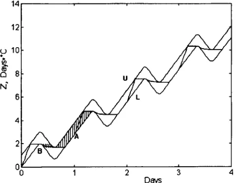
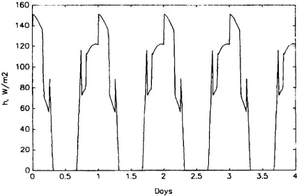
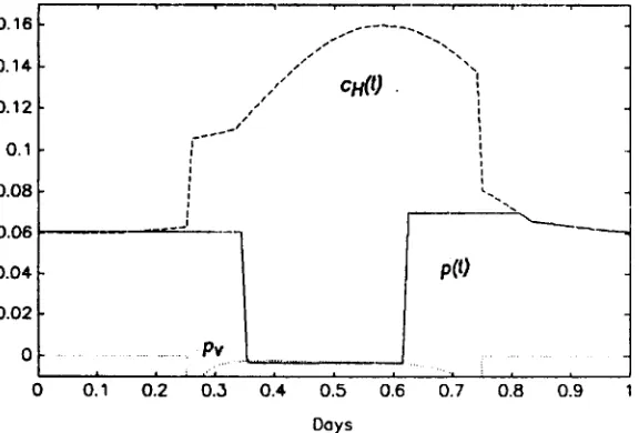
found in Figure 1, where z ( r ) and its constraints (43) are plotted against time, and in Figures

2-6, where T , ( t ) , h ( t ) , q(r) and p ( r ) together with c,, from (26) and -Dc,U*bs/(bs- DUVJ2

from (33) are displayed respectively.

Comparing Figures 1, 5 and 6, we see how the control action corresponds to the optimal

conditions in (26) and (33). Consider 1 day of operation starting at 0040 h. At first p > ~ , ,

giving maximum heating. Then, when C, increases above p , the heating stops. In the late

morning the state hits its lower bound, p jumps downwards to become smaller than the upper

condition for ventilation, (33), and ventilation starts. In the afternoon the upper condition for

ventilation decreases and ventilation stops. A short while afterwards the state touches its upper

NON-LINEAR OPTIMAL GREENHOUSE CONTROL PROBLEM 165 when the state hits and follows its lower constraint, does the heating go on. When the state

follows its lower constraint, we see that p = c H , with p decreasing. This agrees with the

condition of optimality in (37).

It is clearly seen in Figure 1 that heating takes place, i.e. z(t) is increasing, whenever a minimum of the upper z-constraint is less than the next maximum of the lower z-constraint. Ventilation takes place whenever a maximum of the lower z-constraint is larger than the next minimum of the upper z-constraint. Otherwise there will be no heating or ventilation respectively, because non-zero controls decrease the performance criterion. Each pair of such

Figure I . The transformed state :(I) and its upper constraint (marked by U ) and lower constraint (L) from (43) during 4 days. Parts of the sets A and B from Section 4 are striped and dotted respectively

35

30

0

I-

.-

- 25

20

15

0

T-

(I

0.5

--T

2 2.5 3

[image:9.504.133.373.195.381.2]

Days

166 I. IOSLOVICH, P.-0. GUTMAN AND I. SEGINER

‘maximum of the lower z-constraint’ and ‘minimum of the upper z-constraint’ splits the trajectory, since there is no reason to go lower than the ‘minimum of the upper zconstraint’ i.e.

no reason for additional ventilation, and also no reason to go higher than the ‘maximum of the

lower z-constraint’ (additional heating). The initial and final z-values, if they are prescribed, also have to be compared with neighbouring ‘minimum upper’ and ‘maximum lower’ constraint

values. It also follows that since the trajectory is split in such a way, a change in the cost of

heating has no influence on the process of ventilation and vice versa.

From the above it is clear that the set of all feasible points z ( t ) can be divided into two sets:

160

140

120

100 E

‘

80

I

c- 60

4 0

20

(v

\

0

0 0.5 1 1.5 2 2.5

Doys

3 3.5

Figure 3. The heating h ( r ) during 4 days

d

0.4

0.2

0

i

1.5 1

\

I .5 2

Doys

I

i

i

_j

1.5 4

[image:10.504.100.404.196.396.2] [image:10.504.98.403.430.635.2]

NON-LINEAR OITMAL GREENHOUSE CONTROL PROBLEM I67

one set A where on the optimal trajectory

H , ( r ) a O

and one set B where on the optimal

trajectory V,,,(t)20. A rule can now be formulated to determine whether a point z ( t ) belongs to

A or B. Let us consider a feasible point (t, z ( t ) ) . The straight line trajectory emanating from

(t, z(f)) rightwards with dz(t)/dt=O will at some instant f , E [ t ,

f]

either (a) cross the lower z-

bound,'(b) cross the upper bound or (c) not cross any bound at all until the final time f. In the

last case (c) there are three possibilities: (i) the final state

z ( 0

is larger than the prescribed final value 5 , (ii) z ( f ) = 2 or (iii) z ( f )

<

I. Clearly z(f) satisfying (a), or (c)(iii) belongs to the set A,

0.16

0.14

0.12

0.1

0.08

0.06

0.04

0.02

0

o 0.1 0.2 0.3 0.4 0.5 0.6 0.7 0.8 0.9 i

Days

Figun 5. The adjoint variable ( 1 ) during 1 day, together with cH and y.. For periods when the solar radiation s ( r ) > O , yv =

-

Dc,U

4

bs/(bs

-

DUV,)2 (see (26) and (33)); otherwise y , is assigned as zero

0.07

/'

0.05

0 0.5 1

Days

----

\$ I1

-0.005

-0.0 1

0 0.5 1

Days

Figure 6. Zoomed excerpts of Figure 5 of the adjoint variable p ( r ) during I day, together with cH (upper graph) and

[image:11.504.112.400.179.374.2] [image:11.504.183.324.423.621.2]

168 I. IOSLOVICH. P.-0. GUTMAN AND I. SEGINER

z ( t ) satisfying (b) or (c)(i) belongs to B and z ( t ) satisfying (c)(ii) belongs to A

n

B. Parts of

the sets A and B are marked in Figure 1.

Hence in case (a) both the lower and upper z-bounds for the interval [t,

r , ]

may be replaced

by monotonically increasing curves with the decreasing parts of the original bound replaced by constants. In case (b) the bounds can be replaced by monotonically decreasing curves. Similar

simplifications are valid in the remaining cases. In particular, in case (b) when both z ( t ) and

z ( r , ) belong to the upper bound, the whole section of the upper bound for [ I , t , ] can be

replaced by a straight line. A similar statement holds for the lower bound in case (a).

If cq = 0, then, as shown in Reference 2. ventilation is applied only when the costate variable

is zero and it is non-unique. Referring to Figure 1, this would mean that the decreasing z-curve

segments could have been replaced by arbitrary non-increasing curve segments that connect the same neighbouring local maxima and minima of the constraint curves.

5. CONCLUSIONS

The model as formulated in (1) is a first-order approximation of a greenhouse where heating

and ventilation are mutually exclusive. As soon as optimization of humidity and C 0 2

concentration are also considered, this mutual exclusion (15) may not be taken for granted. For the present control problem, which represents many commercial greenhouses, the constraints of the transformed state variable z(t) are calculated on the assumption that the

outside weather is known 4 days in advance; see Figure 1. These constraints are a very useful

guide to optimal control decisions. They may be plotted, as in Figure 1, before the optimal

solution is available, based on the future (expected) weather alone. The plot shows clearly whether and where the optimal solution will touch a constraint. In Figure 1 it would be at a local maximum of the lower bound and at a local minimum of the upper bound. Note that the period between touching events is completely isolated from the rest of the problem and can be solved independently of it. This reduces, in many cases considerably, the solution horizon. In the

example of Figure 1, a weather forecast of at most 17 h is required. If switching between

heating and ventilation is required, z(t) would hit each of the constraints at least once a day. In the example it actually hits each constraint twice a day.

It should also be noted that with given state constraints the optimal trajectory is independent of the values of the cost of heating and cost of ventilation as long as these costs are positive constants. This means that in many cases only a short-term weather forecast is needed to implement on-line a controller based on an optimal solution.

APPENDIX: HEATING AND VENTILATION ARE MUTUALLY EXCLUSIVE

Let us prove the property

q* (t)h" ( t ) = 0 (45)

for the optimal solution q * ( t ) and h*(t). From the Hamiltonian of the original, non-

transformed form (1) it is clear that the part of the Hamiltonian that has to be maximized with

respect to h and q is

F = p ( h + b ~ ) / ( l / + q ) - c , h - ~ , , q (46)

If p s 0, then h = 0 for every q, as both h and q are positive, otherwise F will decrease. If

y B 0, then q = 0 for all values of h, otherwise F will decrease.

NON-LINEAR OPTIMAL GREENHOUSE CONTROL PROBLEM 169 REFERENCES

1. Seginer, I.. ‘Optimal control techniques for energy conservation in controlled environments’, F A 0 CNRE Bull., 2. Gutman P. 0.. P . 4 . Lindberg, I. Ioslovich and I. Seginer, ‘A non-linear optimal greenhouse control problem 3. Pontryagin, L. S., V. G. Boltyansky, R. V. Gamkrelidze and E. F. Mischenko, The Marhenlatical Theory of 4. Krotov, V. F. and V. I. Gurman, The Metho& and Probletns of Optinial Control, Nauka, Moscow, Russia, 1973 5. Bailey, B. 1. and I. Seginer, ‘Optimum control of greenhouse heating’, A m Horr., 245, 512-518 (1989). 6. Seginer. I., C. Gary and M. Tchamichian, ‘Optimal temperature regimes for a greenhouse crop with a

7. Seginer, I., A. Angel, S. Gal and D. Kantz, ‘Optimal C02 enrichment strategy for greenhouses: a simulation study,

8. Leitmann, G., An Introduction to Optimal Conrrof, McGraw-Hill, New York, 1966.

9. Ioffe, A. D. and V. M. Tihomirov, Theory of Extremal Problems, North-Holland, Amsterdam, 1979. 10. B m k e . A., D. Kendrick and A. Meeraus, GAMS: A User‘s Guide, Scientific, Redwood City, CA, 1988.

23, 160-169 (1988).

solved by linear programming’, J . Agric. Eng. Res., 55,335-351 (1993). Oprimal Processes, Wiley-Intencience, New York, 1962.

(in Russian).