http://cmde.tabrizu.ac.ir
Vol. 4, No. 3, 2016, pp. 230-248
Numerical method for solving optimal control problem of the linear differential
systems with inequality constraints
Farshid Mirzaee∗
Faculty of Mathematical Sciences and Statistics, Malayer University, P. O. Box 65719-95863, Malayer, Iran.
E-mail:[email protected],fa [email protected]
Afsun Hamzeh
Faculty of Mathematical Sciences and Statistics, Malayer University, P. O. Box 65719-95863, Malayer, Iran.
E-mail:[email protected]
Abstract In this paper, an efficient method for solving optimal control problems of the linear differential systems with inequality constraint is proposed. By using new adjustment of hat basis functions and their operational matrices of integration, optimal control problem is reduced to an optimiza-tion problem. Also, the error analysis of the proposed method is investigated and it is proved that the order of convergence isO(h4). Finally, numerical examples affirm the efficiency of the proposed method.
Keywords.Adjustment of hat basis functions, Operational matrices, Optimal control, Differential systems, Inequality constraint, Error analysis.
2010 Mathematics Subject Classification.34H05, 49K15, 93C15, 65D25, 65D30. 1. INTRODUCTION
Finding analytic solution for optimal control problems with inequality constraints is dif-ficult so numerical methods to get approximate solutions are important. In deterministic setting, there are many text books for analytic solutions of optimal control problems [1,2,5,
6,16,27,28,29]. Furthermore, numerical schemes for these problems have been provided
in some articles [4,8,12,13,14,15,19,22,33].
Orthogonal functions, often used to solve various problems of dynamic systems. The aim of this technique is reducing these problems to a set of algebraic equations. Typical examples are the block-pulse functions [10], Legendre polynomials [3], Laguerre polynomials [11], Chebyshev polynomials [9] and Fourier series [30].
There are different basic functions for the solution of optimal control problems successfully solve the unconstrained problem such as block-pulse functions [10]. But often results in analytical and computational for solving the optimal control problems with inequality con-straints are difficulties. In recent years, the development of computational techniques for
Received: 25 October 2016 ; Accepted: 3 January 2017.
∗Corresponding author.
solving problems such as hybrid of block-pulse functions and Legendre polynomials [20,31], triangular orthogonal functions [7], B-spline functions [32].
The aim of this paper is developing a numerical scheme based on the adjustment of hat basis functions to solve the optimal control problem of the linear differential systems with inequality constraints. Operational matrices of the adjustment of hat basis functions reduce such problems to those that solve a system of algebraic equations which greatly simplify the problem. Consider the linear differential system
˙
X(t) =K(t)X(t) +F(t)U(t), (1.1)
X(0) =Y, (1.2)
with inequality constraints as
G(t)X(t) +H(t)U(t)≤L(t), (1.3)
whereX(t), U(t)are unknown functions andL(t)is a known function. AlsoK(t), F(t), G(t) andH(t)are matrices of appropriate dimensions.
The aim of this paper is finding the numerical approximation of optimal controlU∗(t)and the corresponding optimal stateX∗(t),0≤t≤T, satisfying Eqs. (1.1)-(1.3) while minimizing the quadratic cost functional
J = ∫ T
0
[
XT(t)Q(t)X(t) +UT(t)R(t)U(t)]dt, (1.4)
whereQ(t)andR(t)are positive semi-definite and positive definite matrices, respectively.
Definitions of adjustment of hat basis functions and their properties are given in Section 2. In Section 3, the adjustment of hat functions are developed to approximate the solution of optimal control problem governed by linear differential systems. In Section 4, the error analysis is proved. In Section 5, the proposed method is used for solving some numerical examples. Finally, Section 6 affords some brief conclusion.
2. DEFINITIONS OF ADJUSTMENT OF HAT BASIS FUNCTIONS AND THEIR PROPERTIES
A set of adjustment of hat functions are defined on[0, T]as [24]
ϕ0(t) =
−1
6h3(t−h)(t−2h)(t−3h) 0≤t≤3h,
0 otherwise,
(2.1)
ifi= 3k−2and1≤k≤n3
ϕi(t) =
1
2h3(t−(i−1)h)(t−(i+ 1)h)(t−(i+ 2)h) (i−1)h≤t≤(i+ 2)h,
0 otherwise,
ifi= 3k−4and2≤k≤n3 + 1
ϕi(t) =
−1
2h3(t−(i−2)h)(t−(i−1)h)(t−(i+ 1)h) (i−2)h≤t≤(i+ 1)h,
0 otherwise,
(2.3)
ifi= 3kand1≤k≤ n3 −1
ϕi(t) =
1
6h3(t−(i−3)h)(t−(i−2)h)(t−(i−1)h) (i−3)h≤t≤ih,
−1
6h3(t−(i+ 1)h)(t−(i+ 2)h)(t−(i+ 3)h) ih≤t≤(i+ 3)h,
0 otherwise,
(2.4)
and
ϕn(t) =
1
6h3(t−(T−h))(t−(T−2h))(t−(T−3h)) (T−3h)≤t≤T,
0 otherwise,
(2.5)
whereh=Tn is a sampling period andn≥3is an integer of multiple three.
Let us divide interval[0, T]into n3 subintervals[ih,(i+ 3)h]wherei = 0,3, ..., n−3, of equal lengths3h. By using the definition of adjustment of hat functions, we have
ϕi(kh) =
1 i=k,
0 i̸=k,
(2.6)
and n ∑
i=0
ϕi(t) = 1.
An arbitrary real functionf(t)on[0, T]can be expanded in an adjustment of hat series as follows
f(t)≃ n ∑
i=0
fiϕi(t) =FTΦ(t) = ΦT(t)F, (2.7)
where
and
Φ(t) = [ϕ0(t), ϕ1(t), ..., ϕn(t)]T, (2.8)
with
fi=f(ih), i= 0,1, ..., n. (2.9)
Also, expand∫0tϕi(s)dsby relation (2.7) in terms of the adjustment of hat basis functions as ∫ t
0
ϕi(s)ds≃ n ∑
j=0
ai,jϕj(t), i= 0,1, ...n. (2.10)
By using relation (2.9), we can compute the coefficientsai,jas follows
ai,j= ∫ jh
0
ϕi(s)ds, i, j= 0,1, ..., n. (2.11)
Now,P is the(n+ 1)×(n+ 1)coefficients matrix with entriesai,j,i, j = 0,1, ..., n, we obtain
P = h 24
0 9 8 9 9 . . . 9
0 p1 p2 p3 p3 . . . p3 0 0 p1 p2 p3 . . . p3 0 0 0 p1 p2 . . . p3 0 0 0 0 p1 . . . p3
..
. ... ... ... ... . .. ...
0 0 0 0 0 . . . p1
(n+1)×(n+1)
,
where
p1=
−195 328 2727
1 0 9
3×3
, p2=
2727 2727 2727
18 17 18
3×3
, p3=
2727 2727 2727
18 18 18
3×3
,
and0based on its location in the matrix, is the3×3zero matrix or 3-vector.
From relations (2.8) and (2.10), we obtain ∫ t
0
Also, we have
Φi(t)Φj(t) =
0 i= 3k, 0≤k≤ n3 and|i−j| ≥4,
0 otherwise and|i−j| ≥3.
(2.13)
Now, from relations (2.8) and (2.13) we have
Φ(t)ΦT(t) = Λ, (2.14)
where matrixΛis shown in page 236.
Therefore, from (2.14) we have ∫ T
0
Φ(s)ΦT(s)ds=Z, (2.15)
where
Z= h 560
128 99 −36 19 0 0 0 0 · · · 0
99 648 −81 −36 0 0 0 0 · · · 0
−36 −81 648 99 0 0 0 0 · · · 0
19 −36 99 256 99 −36 19 0 · · · 0
0 0 0 99 648 −81 −36 0 · · · 0
. .. . .. . .. . .. . ..
0 · · · 0 19 −36 99 256 99 −36 19
0 · · · 0 0 0 0 99 648 −81 −36
0 · · · 0 0 0 0 −36 −81 648 99
0 · · · 0 0 0 0 19 −36 99 128
(n+1)×(n+1)
.
(2.16)
Φ(t)ΦT(t) =
ϕ0(t) 0 · · · 0
0 ϕ1(t) · · · 0
..
. ... . .. ...
0 0 · · · ϕn(t)
(n+1)×(n+1)
. (2.17)
Definition 2.1.For two constant vectorsaT = [a
0, a1, . . . , an]andbT = [b0, b1, . . . , bn], we define
aT ⊙bT = [a0b0, a1b1, . . . , anbn],
Λ
=
ϕ
2 (0
t ) ϕ0 ( t ) ϕ1 ( t ) ϕ0 ( t ) ϕ2 ( t ) ϕ0 ( t ) ϕ3 ( t ) 0 0 0 0 ·· · 0 ϕ0 ( t ) ϕ1 ( t ) ϕ
2 (1
t ) ϕ1 ( t ) ϕ2 ( t ) ϕ1 ( t ) ϕ3 ( t ) 0 0 0 0 ·· · 0 ϕ0 ( t ) ϕ2 ( t ) ϕ1 ( t ) ϕ2 ( t ) ϕ
2 (2
t ) ϕ2 ( t ) ϕ3 ( t ) 0 0 0 0 ·· · 0 ϕ0 ( t ) ϕ3 ( t ) ϕ1 ( t ) ϕ3 ( t ) ϕ2 ( t ) ϕ3 ( t ) ϕ
2(3
t ) ϕ3 ( t ) ϕ4 ( t ) ϕ3 ( t ) ϕ5 ( t ) ϕ3 ( t ) ϕ6 ( t ) 0 ·· · 0 0 0 0 ϕ3 ( t ) ϕ4 ( t ) ϕ
2(4
t ) ϕ4 ( t ) ϕ5 ( t ) ϕ4 ( t ) ϕ6 ( t ) 0 ·· · 0 . .. . .. . .. . .. . .. . .. . .. . .. . .. . .. . .. . .. . .. . .. . .. . .. . .. . .. . .. . .. . .. . .. . .. . .. . .. . .. 0 ·· · 0 ϕn − 6 ( t ) ϕn − 3 ( t ) ϕn − 5 ( t ) ϕn − 3 ( t ) ϕn − 4 ( t ) ϕn − 3 ( t ) ϕ
2 n−
3 ( t ) ϕn − 3 ( t ) ϕn − 2 ( t ) ϕn − 3 ( t ) ϕn − 1 ( t ) ϕn − 3 ( t ) ϕn ( t ) 0 ·· · 0 0 0 0 ϕn − 3 ( t ) ϕn − 2 ( t ) ϕ
2 n−
2 ( t ) ϕn − 2 ( t ) ϕn − 1 ( t ) ϕn − 2 ( t ) ϕn ( t ) 0 ·· · 0 0 0 0 ϕn − 3 ( t ) ϕn − 1 ( t ) ϕn − 2 ( t ) ϕn − 1 ( t ) ϕ
2 n−
1 ( t ) ϕn − 1 ( t ) ϕn ( t ) 0 ·· · 0 0 0 0 ϕn − 3 ( t ) ϕn ( t ) ϕn − 2 ( t ) ϕn ( t ) ϕn − 1 ( t ) ϕn ( t ) ϕ
2 (n
t
)
Theorem 2.1. Let us approximate each of the functions ofa(t)andb(t)by the adjustment of hat basis functions. That is,
a(t)≃ATΦ(t) = ΦT(t)A,
b(t)≃BTΦ(t) = ΦT(t)B.
Then we have
a(t)b(t)≃(AT ⊙BT)Φ(t).
Proof. From (2.17), we have
a(t)b(t)≃ATΦ(t)ΦT(t)B≃AT
ϕ0(t) 0 · · · 0
0 ϕ1(t) · · · 0
..
. ... . .. ...
0 0 · · · ϕn(t) B
= [a0ϕ0(t), a1ϕ1(t), ..., anϕn(t)]B= ΦT(t)
a0 0 · · · 0
0 a1 · · · 0
..
. ... . .. ... 0 0 · · · an
B
=a0b0ϕ0(t) +a1b1ϕ1(t) +...+anbnϕn(t) = [a0b0, a1b1, ..., anbn]Φ(t) = (AT ⊙BT)Φ(t).
Hence, this completes the proof.
3. BASIC IDEA
Firstly, we can rewrite relations (1.1) and (1.2) as
X(t) =Y + ∫ t
0
K(s)X(s)ds+ ∫ t
0
F(s)U(s)ds. (3.1)
Then, consider theith equation of relation (3.1)
xi(t) =yi+ ∫ t
0
∑n
j=0
kij(s)xj(s) + n ∑
j=0
fij(s)uj(s)
ds, (3.2)
withith inequality constraint of (1.3), we have n
∑
j=0
gij(t)xj(t) + n ∑
j=0
hij(t)uj(t)≤li(t). (3.3)
xi(t)≃ΦT(t)Xi=XiTΦ(t),
ui(t)≃ΦT(t)Ui=UT i Φ(t),
yi(t)≃ΦT(t)Yi=YT i Φ(t),
li(t)≃ΦT(t)Li =LT i Φ(t),
(3.4)
gij(t)≃ΦT(t)Gij=GTijΦ(t),
hij(t)≃ΦT(t)Hij=HijTΦ(t),
kij(t)≃ΦT(t)Kij =KijTΦ(t),
fij(t)≃ΦT(t)Fij=FijTΦ(t),
(3.5)
where matricesGij, Hij, KijandFijand vectorsXi, Ui, YiandLiare the adjustment of hat functions coefficients ofgij, hij, kij, fij, xi, ui, yiandli, respectively.
Substituting (3.4) and (3.5) into (3.2) and (3.3), and using Theorem (1) we have
XiTΦ(t)≃Y T i Φ(t) +
n ∑
j=0
(KijT ⊙X
T j )
∫ t
0
Φ(s)ds+
n ∑
j=0
(FijT ⊙U
T j )
∫ t
0
Φ(s)ds,
subject to
n ∑
j=0
(GTij⊙XjT)Φ(t) +
n ∑
j=0
(HijT ⊙UjT)Φ(t)≤LTiΦ(t).
By using (2.12) and replacing≃with=and eliminatingΦ(t), we get
XiT =YiT + n ∑
j=0
(KijT⊙XjT)P+
n ∑
j=0
(FijT ⊙UjT)P, i= 0,1, . . . , n, (3.6)
n ∑
j=0
(GTij⊙XjT) +
n ∑
j=0
(HijT ⊙UjT)≤LTi. (3.7)
The system of linear equations (3.6) and (3.7), can be expressed in the following matrices form
˜
XT −V −W = ˜YT, (3.8)
subject to
˜
A+ ˜B ≤L˜T, (3.9)
where
VT = ∑n j=0(K
T
0j⊙XjT)P ∑n
j=0(K
T
1j⊙XjT)P
.. . ∑n
j=0(K
T
nj⊙XjT)P
, WT = ∑n j=0(F
T
0j⊙UjT)P ∑n
j=0(F
T
1j⊙UjT)P
.. . ∑n
j=0(F
T
nj⊙UjT)P , and ˜ AT =
∑n
j=0(GT0j⊙XjT) ∑n
j=0(GT1j⊙XjT)
.. . ∑n
j=0(G
T nj⊙X
T j)
, B˜T = ∑n
j=0(H0Tj⊙UjT) ∑n
j=0(H1Tj⊙UjT)
.. . ∑n
j=0(H
T nj⊙U
T j ) , and ˜
X = [X0, X1, . . . , Xn]T,
˜
Y = [Y0, Y1, . . . , Yn]T,
˜
whereX,˜ Y˜ andL˜are(n+ 1)2dimensional vectors and
Xi = [Xi0, Xi1, . . . , Xin]T,
Ui= [Ui0, Ui1, . . . , Uin]T,
Kij= [K0
ij, Kij1, . . . , Kijn]T,
Fij= [F0
ij, Fij1, . . . , Fijn]T,
Yi= [Yi0, Yi1, . . . , Yin]T,
Li= [Li0, Li1, . . . , Lin]T
Gij = [G0ij, G1ij, . . . , Gnij]T,
Hij = [Hij0, Hij1, . . . , Hijn]T.
By this method, system of Eq. (3.1) is reduced to system of(n+ 1)2algebraic equations.
Now, we have
J = ∫ T
0
n ∑
i=0
∑n
j=0
xi(t)qij(t)xj(t) dt+
∫ T
0
n ∑
i=0
∑n
j=0
ui(t)rij(t)uj(t) dt.
(3.10)
Let us approximateqij andrijby the adjustment of hat functions as follows
qij(t)≃ΦT(t)Qij=QTijΦ(t),
rij(t)≃ΦT(t)Rij =RTijΦ(t),
(3.11)
where matricesQij andRij are the adjustment of hat functions coefficient matrices ofqij andrij, respectively.
J ≃ n ∑
i=0
∑n
j=0
(XiT ⊙QTij)(
∫ T
0
Φ(t)ΦT(t)dt)Xj
+ n ∑
i=0
∑n
j=0
(UiT ⊙RTij)(
∫ T
0
Φ(t)ΦT(t)dt)Uj
.
By using (2.15) and replacing≃with=and eliminatingΦ(t), we have
J = n ∑
i=0
∑n
j=0
(XiT⊙QTij)ZXj
+
n ∑
i=0
∑n
j=0
(UiT ⊙RTij)ZUj
. (3.12)
Now, we findXandUsuch thatJ(X, U)in (3.12) is minimized subject to the constraints in (3.8) and (3.9). In this paper, the method used to solve the nonlinear constrained optimization problem is based on sequential quadratic programming (SQP) algorithm. SQP is an iterative method for nonlinear optimization. The idea of the SQP methods is to solving the nonlinearly constrained problem using a sequence of quadratic programming subproblems. Also, the approximated solution in each iteration need not be feasible points, since the computation of feasible points in case of the nonlinear constraints may be as difficult as the solution of the nonlinear programming itself [18].
4. ERROR ANALYSIS OF THE PROPOSED METHOD
In this section, we investigate that the rate of convergence of the mentioned approach is
O(h4). We define
∥x(t)∥= sup
t∈[0,T]
|x(t)|. (4.1)
Theorem 4.1. Assume thatX(t) = [X0, X1, . . . , Xn]∈(C4[0, T])n+1and
Xm(t) = [Xm0(t), Xm1(t), . . . , Xmn(t)] =
[∑ni=0X0(ih)ϕi(t),
∑n
i=0X1(ih)ϕi(t), . . . ,
∑n
i=0Xn(ih)ϕi(t)],
be the adjustment of hat functions expansion ofX(t).
Then we have
(i)∀j∥Xj(t)−Xmj(t)∥=O(h4),
Proof. (i)Let
Ek(t) =
Xj(t)−Xmj(t) t∈Ik,
0 t∈[0, T]−Ik,
whereIk ={t|kh≤t≤(k+ 3)h}, k= 0,3, ..., n−3. Then, we obtain
Ek(t) =Xj(t)− n ∑
i=0
Xj(ih)ϕi(t) =Xj(t)−(Xj(kh)ϕk(t)
+Xj((k+ 1)h)ϕk+1(t) +Xj((k+ 2)h)ϕk+2(t) +Xj((k+ 3)h)ϕk+3(t)).
By using third degree interpolation error, we obtain [25]
Ek(t) = (t−kh)(t−(k+ 1)h)(t−(k+ 2)h)(t−(k+ 3)h)
24 .
d4Xj(ηk) dt4 ,
whereηk ∈(kh,(k+ 3)h).
Now consideru(t) = (t−kh)(t−(k+ 1)h)(t−(k+ 2)h)(t−(k+ 3)h). Since,u(t)is a continuous function andIkis compacted, sosupt∈Ik|u(t)|= maxt∈Ik|u(t)|= 2.798h
4.
Also, we have
|Ek(t)| ≤ 1
24|u(t)||
d4Xj(ηk) dt4 |.
Hence, we have
∥E(t)∥=∥Xj(t)−Xmj(t)∥= max
k=0,3,...,n−3tsup∈Ik|Ek(t)| ≤k=0max,3,...,n−30.0867h
4|d4Xj(ηk)
dt4 |.
Then, there is al∈ {0,3, ..., n−3}, where
∥E(t)∥ ≤ max
k=0,3,...,n−30.0867h
4|d4Xj(ηk)
dt4 |= 0.0867h
4|d4Xj(ηl) dt4 |.
Finally, by using relation (4.1), we have
∥E(t)∥ ≤0.0867h4|d
4Xj(ηl)
dt4 | ≤0.0867h 4∥d
4Xj(t)
dt4 ∥. (4.2)
According to relation (4.2), we obtain
∥E(t)∥=O(h4). (ii)From case(i), we have
∥ ∫ t
o
(Xj(s)−Xmj(s))ds∥ ≤
∫ t
o
≤0.0867h4∥d
4Xj(t)
dt4 ∥
∫ t
0
ds= 0.0867h4t∥d
4Xj(t)
dt4 ∥,
sincet∈[kh,(k+ 3)h]≤T, then we have
∥ ∫ t
o
(Xj(s)−Xmj(s))ds∥ ≤0.0867T h4∥
d4X
j(t)
dt4 ∥. (4.3)
According to relation (4.3), we obtain
∥ ∫ t
o
(Xj(s)−Xmj(s))ds∥=O(h4).
Hence, this completes the proof.
5. NUMERICAL EXAMPLES
In this section, we demonstrate the efficiency and accuracy of the proposed method by three examples and obtain the results forn = 15,63. All computations were carried out using a program written in Matlab.
Example 5.1.Consider the minimization of functional [16]
J = 1 2
∫ 1
0
( XT(t)
(
1 0
0 0
)
X(t) +U2(t) )
dt,
subject to
˙ X(t) =
(
0 1
0 −1
) X(t) +
( 0 1
) U(t),
|U(t)| ≤1,
X(0) =
( 0
10 )
.
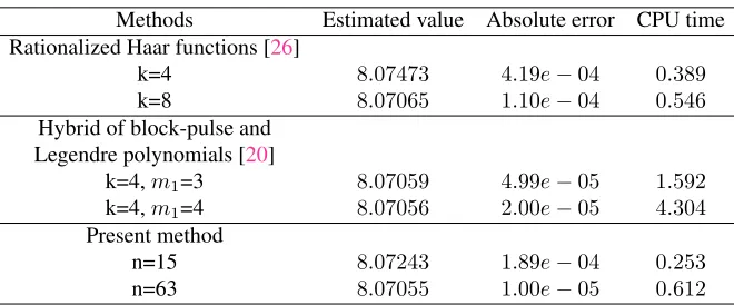
where the optimal control of cost functional isJ = 8.07054. A comparison between the cost functional obtained by the proposed method via the Rationalized Haar functions method [26] and Hybrid of block-pulse and Legendre method [20] is shown in Table 1.
Example 5.2.Consider the minimization of functional [17]
J = ∫ 1
0
( XT(t)
(
1 0
0 0
)
X(t) + 0.005U2(t)
subject to
˙ X(t) =
(
0 1
0 −1
) X(t) +
( 0
1 )
U(t),
X2(t)≤8(t−0.5)2−0.5,
X(0) =
( 0
−1 )
.
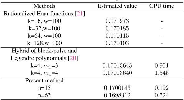
A comparison between the cost functional obtained by the proposed method via the Ratio-nalized Haar method [21] and Hybrid of block-pulse and Legendre method [20] is shown
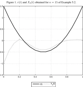
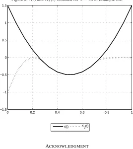
in Table 2. The computational results forX2(t)for n = 15 andn = 63 together with
r(t) = 8(t−0.5)2−0.5are given in Figures 1 and 2.
Table 1.Estimated values and absolute errors of J for Example 5.1.
Methods Estimated value Absolute error CPU time
Rationalized Haar functions [26]
k=4 8.07473 4.19e−04 0.389
k=8 8.07065 1.10e−04 0.546
Hybrid of block-pulse and Legendre polynomials [20]
k=4,m1=3 8.07059 4.99e−05 1.592
k=4,m1=4 8.07056 2.00e−05 4.304
Present method
n=15 8.07243 1.89e−04 0.253
n=63 8.07055 1.00e−05 0.612
Example 5.3.Consider the minimization of functional [23]
J = ∫ 1
0
subject to
˙ X(t) =
(
0 1
0 0
) X(t) +
( 0 1
) U(t),
X1(t)≤0.15,
X(0) =
( 0
1 )
, X(1) =
( 0
−1 )
.
A comparison between the cost functional obtained by the proposed method via the Gradient-restoration method [23] is shown in Table 3.
Table 2.Estimated values of J for Example 5.2.
Methods Estimated value CPU time
Rationalized Haar functions [21]
k=16, w=100 0.171973
-k=32,w=100 0.170185
-k=64, w=100 0.170115
-k=128,w=100 0.170103
-Hybrid of block-pulse and Legendre polynomials [20]
k=4,m1=3 0.17013645 0.951
k=4,m1=4 0.17013640 1.545
Present method
n=15 0.1700143 0.192
Figure 1.r(t)andX2(t)obtained forn= 15of Example 5.2.
0 0.2 0.4 0.6 0.8 1
−1.5 −1 −0.5 0 0.5 1 1.5
r(t) X
2(t)
Table 3.Estimated values of J for Example 5.3.
Methods Estimated value CPU time
Gradient-restoration [23]
N=16 5.927
-Present method
n=15 5.8451 1.025
n=63 5.7346 1.923
6. CONCLUSION
Figure 2.r(t)andX2(t)obtained forn= 63of Example 5.2.
0 0.2 0.4 0.6 0.8 1
−1.5 −1 −0.5 0 0.5 1 1.5
r(t) X
2(t)
ACKNOWLEDGMENT
The authors are very thankful to the reviewers and the editor of this paper for their con-structive comments and nice suggestions, which helped to improve the paper.
REFERENCES
[1] R. E. Bellman, Dynamic programming, Princeton University Press, Princeton, NJ, 1957.
[2] R. E. Bellman, S. E. Dreyfus, Applied dynamic programming, Princeton University Press, Princeton, NJ, 1962. [3] R. Y. Chang, M. L. Wang, Shifted Legendre series direct method for variational problems, Journal of
Opti-mization Theory and Applications, 39 (1983), 299-307.
[4] H. R. Erfanian, M. H. Noori Skandari, Optimal control of an HIV model, The Journal of Mathematics and Computer Science, 2 (2011), 650-658.
[5] W. H. Fleming, C. J. Rishel, Deterministic and stochastic optimal control, Springer-Verlag, 1975. [6] W. H. Fleming, H. M. Soner, Controlled markov processes and viscosity solutions, Springer, 2006.
[7] Z. Han, S. Li, Q. Cao, Triangular orthogonal functions for nonlinear constrained optimal control problems, Journal of Applied Sciences, Engineering and Technology, 12 (2012), 1822-1827.
[8] E. Hesameddini, A. Fakharzadeh Jahromi, M. Soleimanivareki, H. Alimorad, Differential transformation method for solving a class of nonlinear optimal control problems, The Journal of Mathematics and Computer Science, 5 (2012), 67-74.
[9] I. R. Horng, J. H. Chou, Shifted Chebyshev series direct method for solving variational problems, International Journal of Systems Science, 16 (1985), 855-861.
[11] C. Hwang, Y. P. Shih, Laguerre series direct method for variational problems, Journal of Optimization Theory and Applications, 39 (1983), 143-149.
[12] H. M. Jaddu, Direct solution of nonlinear optimal control problems using quasilinearization and Chebyshev polynomials, Journal of the Franklin Institute, 339 (2002), 479-498.
[13] A. Jajarmi, N. Pariz, S. Effati, A. V. Kamyad, Infinite horizon optimal control for nonlinear interconnected Large-Scale dynamical systems with an application to optimal attitude control, Asian Journal of Control, 15 (2013), 1-12.
[14] B. Kafash, A. Delavarkhalafi, S. M. Karbassi, Application of Chebyshev polynomials to derive efficient algo-rithms for the solution of optimal control problems, Scientia Iranica, 19 (2012), 795-805.
[15] B. Kafash, A. Delavarkhalafi, S. M. Karbassi, Application of variational iteration method for Hamilton-Jacobi-Bellman equations, Applied Mathematical Modelling, 37 (2013), 3917-3928.
[16] D. E. Kirk, Optimal control theory an introduction, Prentice-Hall, Englewood Cliffs, 1970.
[17] D. L. Kleiman, T. Fortmann, M. Athans, On the design of linear systems with piecewise-constant feedback gains, IEEE Transactions on Automatic Control, 13 (1968), 354-361.
[18] D. G. Luenberger, Y. Ye, Linear and Nonlinear Programming, New York, Springer, 2008.
[19] K. Maleknejad, H. Almasieh, Optimal control of Volterra integral equations via triangular functions, Mathe-matical and Computer Modelling, 53 (2011), 1902-1909.
[20] H. R. Marzban, M. Razzaghi, Hybrid functions approach for linearly constrained quadratic optimal control problems, Applied Mathematical Modelling, 27 (2003), 471-485.
[21] H. R. Marzban, M. Razzaghi, Rationalized Haar approach for nonlinear constrined optimal control problems, Applied Mathematical Modelling, 34 (2010), 174-183.
[22] S. Mashayekhi, Y. Ordokhani, M. Razzaghi, Hybrid functions approach for nonlinear constrained optimal control problems, Communications Nonlinear Science and Numerical Simulation, 17 (2012), 1831-1843. [23] A. Miele, Gradient algorithms for the optimization of dynamic systems, Control and Dynamic Systems, 16
(1980), 3-52.
[24] F. Mirzaee, A. Hamzeh, A computational method for solving nonlinear stochastic Volterra integral equations, Journal of Computational and Applied Mathematics, 16 (2016), 377-427.
[25] S. Nemati, P. M. Lima, Y. Ordokhani, Numerical solution of a class of two-dimensional nonlinear Volterra in-tegral equations using Legendre polynomials, Journal of Computational and Applied Mathematics, 242 (2013), 53-69.
[26] Y. Ordokhani, M. Razzaghi, Linear quadratic optimal control problems with inequality constraints via rational-ized Haar functions, Dynamics of Continuous, Discrete and Impulsive Systems Series B, 12 (2005), 761-773. [27] A. B. Pantelev, A. C. Bortakovski, T. A. Letova, Some issues and examples in optimal control, MAI Press,
Moscow, 1996.
[28] E. R. Pinch, Optimal control and the calculus of variations, Oxford University Press, London, 1993. [29] L. S. Pontryagin, The mathematical theory of optimal processes, Interscience, John Wiley and Sons, 1962. [30] M. Razzaghi, M. Razzaghi, Fourier series direct method for variational problems, International Journal of
Control, 48 (1988), 887-895.
[31] M. Razzaghi, J. Nazarzadeh, A collocation method for optimal control of linear systems with inequality con-straints, Mathematical Problems in Engineering, 3 (1998), 503-515.
[32] Y. E. Tabrizi, M. Lakestani, Direct solution of nonlinear constrained quadratic optimal control problems using B-spline functions, Kybernetika, 51 (2015), 81-98.