ijgt.ui.ac.ir
ISSN (print): 2251-7650, ISSN (on-line): 2251-7669 Vol. 7 No. 4 (2018), pp. 27-40.
c
⃝2018 University of Isfahan
www.ui.ac.ir
MEASURING CONES AND OTHER THICK SUBSETS IN FREE GROUPS
ELIZAVETA FRENKEL∗AND VLADIMIR N. REMESLENNIKOV
Communicated by Evgeny Vdovin
Abstract. In this paper we investigate the special automata over finite rank free groups and estimate asymptotic characteristics of sets they accept. We show how one can decompose an arbitrary regular subset of a finite rank free group into disjoint union of sets accepted by special automata or special monoids. These automata allow us to compute explicitly generating functions,λ−measures and Cesaro measure of thick monoids. Also we improve the asymptotic classification of regular subsets in free groups.
1. Introduction
This paper continue the series of papers written by different authors [2,1,6,7,8]. More specifically,
we expand the results of [9] and give their proves. We return to the question of asymptotic classification
of regular subsets in finite rank free groups, thus being motivated by needs of universal algebraic
geometry. Namely, having in mind the notion of an A−dimension function over arbitrary algebraic
structure introduced by the second author and its applications in different algebraic systems (see [3]),
we have started to prepare the algebraic and algorithmic foundations for a suitable dimension function
in group theory. In particular, in a sequel paper we are going to present such an algorithm for regular
subsets of finite rank free groups over certain groupA. However, the existing asymptotic classification
of sets, appeared first in [2] and then refined in [1] does not allow us to fulfill this task. To reveal the
problem, we formulate these results (see Section2 for definitions):
MSC(2010): Primary: 20F05; Secondary: 05C05.
Keywords: Free group,λ−measure, regular subset, special automaton, thick monoid. Received: 30 March 2016, Accepted: 06 May 2017.
∗Corresponding author.
DOI:http://dx.doi.org/10.22108/ijgt.2017.21479
Theorem 1.1. [2,1]Let F be a finite rank free group. Then
1) every regular subset ofF is either thick or exponentially negligible;
2) a regular subset of F is thick if and only if its prefix closure contains a cone.
As we shall see below, all the necessary computations can be easily done in the case of regular
exponentially negligible sets. The missing bit consists in more specific characterisation of thick sets
and in finding the way to distinguish between them in a finer way. The present paper covers these
problems.
The following theorem adds to our knowledge on how does the thick sets look like; these new details
turn out to be crucial as we shall show in section 4:
Theorem 3.8. A regular subset R of F is thick if and only if it contains a subset w◦T, with T
being a thick monoid and w∈F.
Another important results of the current paper concerns new algorithms for the computation of the
generating functions and Cesaro measure of sets recognised by so-called special automata and thick
monoids. The algorithms we suggest appears to be easier with respect to the older ones.
Now, a few words on the structure of the paper. In Section2we give some basics on regular sets and
recall techniques for measuring subsets in a free group F and the asymptotic classification of regular
sets. In subsection 2.2 we also provide Algorithm I for computation of the generating function of a
regular set by means of linear algebra.
Section 3starts with the definition of a special automaton over monoid and group. Further on we
prove that every regular subsetL of a finite rank free groupF can be represented as a finite disjoint
union of languages accepted by certain type of automata (see Proposition 3.1), which is going to be
crucial property of the special automata in a context of both current paper and the construction of a
dimension function in free groups. In Lemma3.3we also show how one can split the sets accepted by
special automata, which leads to the notion of a thick monoid.
Further in this section we analyse the structure and compute the most important asymptotic
charac-teristics of thick monoids: the generating function and the Cesaro measure among the most important
of them (see Proposition 3.6 and Lemma 3.7). In Theorem3.8 we improve already mentioned result
on the asymptotic classification of regular sets. We conclude Section 3 with Algorithm II computing
λ−measure of a negligible set accepted by a special automaton.
The next Section4is dedicated to computations and also it reassumes the results from above.
Pre-liminary calculations made in Lemma4.1allows us to compute the generating function of an arbitrary
double-based cone (see Theorem 4.2). We want to emphasize that this is a crucial theorem for all
the paper, interesting per se, applied in Lemma 3.7, and having a lot of structural and
computa-tional consequences. In particular, Theorem 4.2 reduces Algorithm I to much more straightforward
2. Regular sets in free groups
In this section we recall the main definitions and tools of particular interest for our purposes.
2.1. Regular sets: some properties. We assume that the reader is familiar with basic facts on
regular sets in monoids and groups (described in details, for example, in [4,12]). LetX={x1, . . . , xm}
be an alphabet and define Σ to be the letters of X with their formal inverses: Σ = X∪X−1. Let
F =F(X) be the free group generated byX. Afinite state automaton Ais a quintuple (S,Σ, δ, I, Z),
whereS is a finite set of states, Σ is an alphabet,I ⊂S is the (non-empty) set of initial states,Z ⊆S
is the set of final states, and δ is a set of arrows with labels in the enlarged alphabet Σ∪ε (here ε
is assumed not to lie in Σ). Further, a deterministic automaton can be considered a special case of
a finite state automaton, with no arrows labelled ε, the only one initial state and each state being
the source of exactly one arrow with any given label from Σ. By the Kleene-Rabin-Scott theorem,
all regular subsets over Σ (i.e. the closure of finite subsets of free monoid over Σ under the rational
operations) are exactly the sets accepted by a finite state automaton over Σ∪ε, or, equivalently,
accepted by a deterministic automaton over Σ. The language accepted by an automaton A we shall
denote by L=L(A).
2.2. Multiplicative measures: basics and first algorithms. We denote by |f| the length of an
element f ∈ F, and let Sk ={w ∈F | |w|=k} denote the sphere of radius k in F. We consider a
subset R of F, and denote by fk(R) = |R|S∩kS|k| the frequency of elements from R among the words of
lengthk inF.
λ−measure. An important measuring tool in F is the so-called frequency measure, introduced in
[2] and studied in [6] and [7]. By definition,
λ(R) =
∞
∑
k=0
fk(R).
A subset R⊆F is calledλ-measurable, if λ(R) <∞, andexponentially λ−measurableif there exists
a positive constant δ <1 such that fk(R)< δk for big enough k. We adjuste this measure to obtain
λ∗(R) = 2m2m−1λ(R).
Generating function. One can consider the (frequency) generating function for R as a formal
series inR[[t]]: gR(t) =
∑∞
k=0fk(R)tk. We shall also use theadjustedversion of this function: g∗R(t) =
2m
2m−1·gR(t). In case of regular subsets ofF the generating function can be described in a very concise form:
Theorem 2.1. For a regular set R ⊆F the function gR(t) is a rational function of t with rational
coefficients and either
• has a simple pole att= 1 (in this case R is thick1).
In particular,
(2.1) Res1gR(t) =−µ0(R).
Recall that a regular set is called thick if the parameter µ0(R) defined by formula (2.1) is strictly
positive. This parameter µ0(R) is called Cesaro density of R. We use often the following simple
properties of the generating function: suppose R1 and R2 are regular subsets ofF. Then
(1.) If R = R1 ∪R2, then the corresponding generating function can be computed as gR(t) =
gR1(t) +gR2(t)−gR1∩R2(t).
(2.) IfR=R1◦R2, thengR(t) =gR1(t)g∗R2(t).
Now we describe the first algorithm for calculation of the generating function for an arbitrary
regular subset of a finite rank free group F. This algorithm is previously known (see, for example,
[2]), although it was not directly formulated there.
Algorithm I computing the frequency generating function gR(t) for a regular set R.
Indeed, let A= (S,Σ, δ, I, Z) be an automaton such that|S|=nand let Abe it’s adjacency matrix,
i.e. n×n matrix with entries aij such that each aij corresponds to the number of arrows from the
stateito the statej. Clearly, the number of different paths of lengthkfromitoj is equal to (Ak)i,j.
Denote by R the subset ofF accepted byA.
Algorithm I:
1. Given an automatonA, compute the entriesaij,i, j= 1, . . . , nof the adjacency matrix A.
2. Compute the entriesbij of the fundamental matrix B =tA(E−tA)−1 of A, with the entries
bij from the ring of formal power seriesR[[t]].
3. The generating functiongR(t) is equal to
∑
i∈I,j∈Z bij.
One of the disadvantages of the Algorithm I is that step [2.] involves the matrix inversion, and
it makes the algorithm hardly implementable with the size of automaton n big enough. However,
computation of the generating function can be significantly simplified for a wide class of regular sets.
In what follows we introduce this type of sets and describe their structure along with the improved
algorithm for computation of g(t). Now, using Algorithm I and the properties above, we compute
generating function for certain regular subsets of F. We also calculate the corresponding values of
Cesaro densityµ0(R) (defined by formula (2.1)).
Example 2.2. (1) The entire free group F has gF(t) =−t−11 and µ0(F) = 1.
(2) For a set R=F♯=F\ {1} we have g
R(t) = t−−t1 while µ0(F♯) = 1.
1The rationality ofg
R(t) for regular sets is well known (see for instance [5]; it follows also from Algorithm I forgR(t)
(3) Let R be a cone2 C(w) or R=C[w], and let |w|=r. Then gR(t) = 2m(2m1−1)r−1 ·− tr t−1,and
µ0(R) =
1
2m(2m−1)r−1.
(4) If R=F \Br−1, then gR(t) = −t r
t−1, and µ0(R) = 1.
(5) For a subgroupH < F(X)of all words of even length direct calculations of frequency generating
functions gives gH(t) = 1−1t2,and therefore µ0(H) = 1 2.
3. Special automata over free groups and monoids
In this section we investigate one of the central concepts of this paper, i.e. special automata over
monoids and groups. We show in Proposition 3.1 that every regular set in a free group can be
decomposed into finite union of subsets accepted by special automata.
3.1. Definitions. Let A= (S,Σ, δ, i0, Z) be a deterministic automaton. A is called special over the
monoid Σ∗ if
a. The initial vertex has no inedges;
b. There is only one final statez0 ∈Z;
c. Adoes not contain inaccessible states;
d. For every states∈S there is a direct path fromsto the final state z0;
e. For any state s∈S, all arrows which enter s have the same labelx ∈Σ (we shall say, s has
type x).
In order to adjust the notion of speciality to groups, we impose an additional constraint on automata.
Namely, let F be the free group, and Abe a special automaton. Suppose also that
f. For any statesof type xin A, all arrows exiting from scannot have label x−1.
A is aspecialautomaton over the group F, if it satisfies the conditions (a)–(f).
In what follows we also shall use a notion of a special monoid. Namely, a monoidM is calledspecial
if it is accepted by a finite automata A withi0=z0, satisfying conditions (b) – (f).
3.2. Decomposition into special automata.
Proposition 3.1. Let L be a regular language in F. Then there exist a finite number of automata
A0, . . . ,Ak such that
• L is a disjoint union of languagesL0 =L(A0), . . . , Lk=L(Ak) in F: L=L0⊔L1⊔ · · · ⊔Lk; • every Li is either accepted by a special automaton or a special monoid.
Proof. SinceLis regular inF, it is accepted by a finite automatonA. Although we can assume thatAis
deterministic automaton, it will be more convenient for us to start with a non-deterministic one, which
accepts L as a language of reduced words, satisfies (c) (it is always possible, see [10]), but, probably,
hasε−transitions and more than one initial state. Therefore,Ahas a formA= (S,Σ∪ε, δ, I, Z). We
begin with an application of Rabin-Scott powerset construction (see [13] for details). As an output
of this procedure, we obtain an automaton A′ = (S′,Σ, δ′, i0, Z′), which does not have ε-transitions
and has only one initial state i0 without inedges, as required. As a by-product of the construction,
we have conditions (c) and (d) satisfied. Further, because we have started from the automaton A
which does not have consecutive x, x−1(x ∈ Σ) transitions, A′ does not have these transitions as
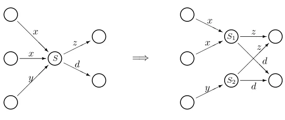
well. Nevertheless, it might happen that A′ has more than one final state and some states ofS′ have
incoming edges with different labels. In the latter case we split the states of A′ as it is shown on
figure 1:
=⇒ m m m m m m m m m m m m m -@ @ @@R
HHHj * * * HHHj -@ @ @@R
S S2 S1 y x x d z y x x d d z z
Figure 1. Splitting the states of the automatonA′.
The output of the splitting procedure we shall callA′′= (S′′,Σ, δ′′, i0, Z′′). IfA′′has only one final
state z0 ̸=i0, then it is special over F. IfZ′′ ={z0} and i0 =z0, then L(A′′) is a special monoid by
definition and due to (f). Suppose now Z′′ = {z0, . . . , zk}, with k ≥ 1. For every zi ∈ Z′′ consider
the maximal connected subgraph Ai = (Si,Σ, δi, i0, zi) of A′′ such that Si ⊂S′′ and δi ⊂δ′′ induced
by the paths of arrows from i0 to zi; obviously, there are two options for Ai: either Ai has distinct
initial and finale state and therefore Ai is special, or initial and final states conincide and so L(Ai)
is a monoid . Since L =L(A′′) and A′′ satisfies (c), (d), clearly, L =L(A0)∪L(A2)∪ · · · ∪L(Ak).
Moreover, this union is disjoint since Li∩Lj ̸=∅ implies existence of paths of arrowsp1, p2 such that
p1 = i0v1· · ·vszi ∈ A′′ and p2 = i0u1· · ·urzj ∈ A′′ for zi ̸= zj, with the label δ′′(p1) = δ′′(p2), a
contradiction with A′′ being deterministic. □
Remark 3.2. Notice that the numberk and subsetsLi for different decompositions ofLcan vary. On
the other hand, supposeL=L0⊔L2⊔· · · ⊔Lk andL=M0⊔M2⊔· · ·⊔Ms are different decomposition
of a regular set L as in Proposition 3.1. Then by property (1.) of the generating functions we have
gL0(t) +· · ·+gLk(t) =gL(t) =gM0(t) +· · ·+gMs(t).
3.3. Further splitting of subsets in free groups. A special automaton satisfying (a)–(f) in turn
Lemma 3.3. Let R=R(A) andA= (S,Σ, δ, i0, z0) be a special automaton over F. Then there exist
regular languages R1, R2, R3 ⊂ F such that Rj are accepted by Aj = (S,Σj, δj, ij, zj), A1 is special
over F and
1. if A has at least one arrow exitingz0, then R2 is non-empty andi2=z2, while i3̸=z3 and
(3.1) R =R1◦R2 is unambiguos;
(3.2) R2 = 1⊔R3⊔(R3◦R3)⊔(R3◦R3◦R3)⊔ · · ·;
(3.3) gR(t) =gR1(t)g∗R2(t); λ(R) =λ(R1)λ∗(R2).
2. if there is no arrows exitingz0, thenR2=R3 =∅,R=R1,λ(R) =λ(R1), andgR(t) =gR1(t).
Proof. Although the construction of sets R1, R2, R3 and their λ−measures appears in [2] and [7], we
shall widely use these sets and automata in what follows, and therefore we repeat briefly the necessary
computations (see also Example 3.5and its illustrations in figures 2,3,4(a),4(b)).
Suppose that the final state of A does not have exiting arrows. Then we leave A as it is, and,
clearly, [2.] holds.
Let nowz0 has at least one exiting arrow. In this case the special automatonA1 accepting R1 can
be obtained from A by removing all arrows exiting from z0; we take i1 = i0 and z1 = z0. Let us
consider the automaton A2 accepting R2 ̸=∅ formed by all states accessible from the state z0, with
the same arrows between them as in A; we takez0 for the bothi2 and z2. If nowu∈R1 andv ∈R2,
then the word uv is reduced and λ(uv) = λ(u)λ∗(v). Therefore, the presentation of R in the form
R =R1◦R2 is unambiguous. Indeed, letw∈R can be written in two different forms as u1◦v1 and
u2◦v2, where u1, u2 ∈ R1 and v1, v2 ∈ R2. Assume that |u1|> |u2|(otherwise consider the pair v1
and v2), and let h =u−21u1 ∈F be readable in A. Notice that h starts atz0 sinceu2 is accepted by A1 and ends at z0 because A1 accepts u1. Therefore, h is accepted by A2, a contradiction with the construction of A1. The estimates onλ(R) and gR(t) now follow immediately from the construction
(frequencies assigned to arrows in A1,A2 the same as they were in A) and formula (2.).
Further, we transform the automaton A2 by splitting the final state z2 =z0 into separate initial
state i3 (with no arrows entering it, and those arrows which were exiting z2 now exiting i3), and the
final state z3 (with no arrows exiting z3, and those arrows which were entering z0 now entering z3).
Then, clearly, (3.2) holds. □
Corollary 3.4. Let R = R(A) and A = (S,Σ, δ, i0, z0) be a special automaton over F, and let
R1, R2, R3 ⊂ F be regular languages such that R1 is accepted by a special automaton over F, R2 is
non-empty set such that its initial and the final state coincide, R3 is accepted by a special automaton
over F; R = R1 ◦R2, and R2 satisfies (3.2) as in lemma above. Then the subset R2 of F is the
free special monoid generated by {wi|i∈ I}, where wi ∈F are words in R3 and wi can be computed
Proof. The automaton A2 constructed in the proof of Lemma3.3 hasi2 =z2, and its final vertex z2
is of x−type, for some x∈Σ. The condition (f) provided by the speciality of A guarantees that the
arrow labelled x−1 cannot exit from i
2. Therefore, ifu1, u2 are accepted by A2, then u1u2 =u1◦u2. In particular, using the further splitting ofR2, one can express everyui as a reduced product of wi’s
accepted by (non-empty) R3. Since the identity belongs to R2, A2 accepts the free special monoid
with generators wi, i∈I. □
The subsets and automata described in Lemma 3.3, claim 1. are of particular interest for us.
Regular setsR⊆F of such form we shall callsaturated. SetsR1, R2, andR3 in the splitting defined in
this lemma we shall call a set of first, second, andthird type, respectively. In what follows, we use the
notations A1,A2,A3 for the splitting of arbitrary automatonA and R1, R2, R3 for the corresponding
regular sets exclusively in a sense of Lemma 3.3. We provide an example of such automata and sets
below.
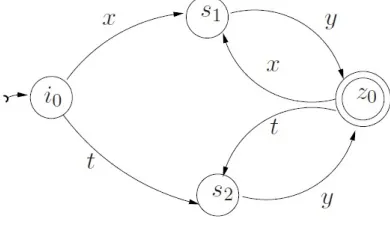
Example 3.5. Let Σbe an alphabet x, y, t, z and the inversion is given by the rule t→x−1, z →y−1
(so X ={x, y}). Consider the special automaton A (the arrow with a tale corresponds to the initial
state, and the finale state is drawn as a double circle).
Figure 2. The special automaton A.
Clearly, R=R(A) is generated by the following regular expression:
R=xy((x−1y)∗(xy)∗)∗∪xy((xy)∗(x−1y)∗)∗⊔
⊔
x−1y((xy)∗(x−1y)∗)∗∪x−1y((x−1y)∗(xy)∗)∗.
The set of first type R1 can be read off by the automaton A1 shown in figure 3; therefore, R1 =
Figure 3. The special automaton A1.
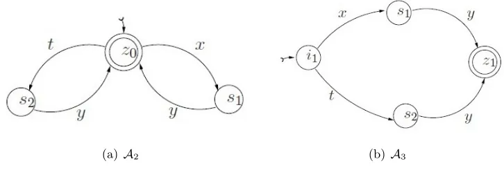
The sets of second type R2 = (
(xy)∗(x−1y)∗)∗ and third type R3 =xy∪x−1y with their automata A2 andA3. Clearly, the elements w1 =xy, w2 =x−1y provides a set of generators for the monoid R2
(see Corollary 3.4).
(a)A2 (b) A3
Figure 4. The automata A2,A3.
3.4. Thick semigroups and cones. We want to classify the subsets accepted by special automata
overF by modulo of their measure. This classification requires recalling of the notion ofX−complete
automaton, which was already used in [2] and [6] for analogous purposes. Let A = (S,Σ, δ, i0, z0)
be a special automaton satisfying the conditions (a)–(f). A is called Σ−complete if for every state
s ∈ S ∖{i0} of type x ∈ Σ every label from Σ∖{x−1} is present on one of the arrows exiting
from s and exactly |Σ| arrows exits from i0. Further, letR2 be a regular set of the second type and A2 = (S,Σ, δ, z0, z0) be the corresponding automaton. A2is called Σ−completeif for every states∈S of type x all arrows labeled by Σ∖{x−1} exit from s. Otherwise A (or A2) is not Σ−complete (for
instance, the automaton A in Example 3.5, as well as A1,A2, and A3 are not Σ−complete). The
following proposition shows that the λ−measure can be easily estimated in the latter case.
Proposition 3.6. Let A be a special automaton satisfying the conditions (a)–(f ), and R = L(A)
be a saturated set such that R = R1 ◦R2 is the splitting of the form (3.1), with R1 = L(A1) and
Proof. IfAis Σ−complete, then only one ofA1,A2can be Σ−complete sinceR1◦R2is unambiguos by
Lemma3.3. Moreover, ifA2 is Σ−complete for the corresponding Σ−complete automatonA, thenA1
is not Σ−complete at the state z0. Thus, we can assume that preciselyA2 is not Σ−complete. Then
R=L(A) isλ−measurable by Theorem 3.4 in [2]. SinceRis regular, it is exponentiallyλ−measurable
by asymptotic classification of regular sets ([2,1]). □
If, on the other hand, A is Σ−complete, then we can improve some previously known results on
classification of regular subsets in free groups. Namely, letR2 be a regular subset ofF of second type
accepted by the automaton A2. According to Corollary 3.4, R2 = L(A2) forms a (special) monoid,
and ifA2is Σ−complete, we shall callR2thick. An interesting fact about thick monoids is that we can
describe them in terms of double-based cones. We recall that the coneC(w) is the set of all elements
in F containing w as initial subword. In what follows we also shall be interested in a symmetric
notion of a cone with a right-hand side handle, i.e. the set of all words in F that terminates with w
(we denote this sort of cones byC[w]). Another member of this family is thedouble-based cone with
(nontrivial) handles w1, w2, consisting of all words inF of the form w1◦f ◦w2, f ∈F. Notice that
all three types of cones are regular in F (see, for example, Corollary 3.15 [8]). Let us consider the
generalized x-coneC(Y, x),x∈Σ, i.e. the union of double-based cones of the form ⊔
y∈Σ:y̸=x−1C(y, x).
The following technical observation regarding generalized cones give us first examples of thick
monoids:
Lemma 3.7. Let C(Y, x) be the generalized x−cone,x∈Σand M =C(Y, x)∪ {1}. Then
1. C(Y, x) =C[x]∖C(x−1, x), and M is a thick monoid;
2. gM(t) = (2m−1)t 2
4m2(1−t) + 1 +
t
2m + t2
4m2 +
t3
2m(2m−1−t), and
3. µ0(M) =
2m−1 4m2 .
Proof. The proof of 1. follows from the definitions of cones and thick monoids, while Example2.2(3)
and Lemma 4.1[3.], [4.] below provide estimates on the generating function and the Cesaro density
given in [2.] and [3.]. □
Now we are ready to refine the asymptotic classification of regular sets inF (see Introduction and
Theorem 3.4 [2] for comparison).
Theorem 3.8. A regular subset R ofF is thick if and only if it contains a subsetw◦T, with T being
a thick monoid and w∈F.
Proof. Clearly, every set of the formw◦T is regular and thick (where 1◦T, by definition, stands for
T). Suppose nowRis regular and thick. We decomposeRinto a finite number of subsets as in Lemma
3.1. Since a finite union of exponentially λ−measurable subsets is exponentially λ− measurable (see,
for example, Proposition 4.1 [6]), without loss of generality one can suppose that R is accepted by a
R is a set accepted by a special automaton. In this case we apply Lemma3.3to procure a pair of sets
R1 andR2 of corresponding types, withR2 being Σ−complete by Proposition3.6. SinceR=R1◦R2,
the set R contains a subsetw◦R2, withw∈R1. This completes the proof. □
3.5. Computing λ−measure of regular sets. Another immediate consequence of Lemma 3.3and
Proposition3.6 is an algorithm for computation of λ−measure of exponentially negligible regular set
R accepted by a special automaton A. We assume that our reader is familiar with the concept of
discrete-time Markov chain and refer to [11] as one of the fundamental manuals on this subject.
Let A = (S,Σ, δ, i0, z0) be a special automaton over F and let R = R(A) be a λ−measurable
regular set. We split A into A1, A2 and A3, obtaining regular sets R1, R2 and R3 (without loss of
generality, one can consider the case when all these sets are non-empty). Further, due to formula (3.3)
and Proposition3.6, it is enough to calculate the value of λ−measure forR3, accepted by the special
automaton A3 = (S3,Σ, δ3, i1, z1).
Consider a finite Markov chain Mwith the same states as inA3 together with an additional dead
state D. We set transition probabilities fromz1 to z1 and from D toD being equal 1. Every arrow
from a state s in A3 gives the corresponding transition from the state s in M which we assign the
transition probability 1
2m−1. If at some state s of type x in A3 there is no exiting arrow labeled
y∈Σ∖{x−1}, we make a transition fromstoDinMassigning it the probability 1
2m−1. We take the stochastic vector being zero everywhere except the state i1 (so it have the only nontrivial entry
1 at the state i1). This complete the description of the Markov chainM. Clearly, the states z1 and
D of Markov chain M are absorbing, and all other states are transient. Obviously, P(z1) = λ(R3),
and it was shown in [2,6] that λ(R3) <1 for any λ−measurable set R. Therefore, one can calculate
λ(R2) using formula (3.2). A similar argument allows to computeλ(R1), and so we are done. Thus,
the Markov chain Mprovides us with the following algorithm for computation of λ(R).
Algorithm II: LetA be a special automaton andR =R(A) beλ−measurable.
1. SplitAinto A1,A2,A3 as in Lemma 3.3.
2. Construct Markov chains forA1= (S1,Σ, δ1, i0, z0) andA3 = (S3,Σ, δ3, i1, z1).
3. Calculate the probabilitiesP(z0) and P(z1); soλ(R1) =P(z0) andλ(R3) =P(z1).
4. Computeλ(R2) =
∞
∑
i=0
Pi(z
1)<∞.
5. Finally, computeλ(R) =λ(R1)·λ∗(R2).
4. Computations
In this section we carry out all necessary measurements of double-based cones and thick monoids.
4.1. Generating functions and Cesaro density of double-based cones. This technical but
crucial lemma will supply us with data about generating function and values of Cesaro density for
double-based cones.
1. fk(C(a, b)) = fk(C(c, d)) and therefore gC(a,b)(t) = gC(c,d)(t) for all a, b, c, d in Σ such that
ab̸= 1, cd̸= 1. Further, fk(C(a, a−1)) =fk(C(b, b−1))for arbitrary a, b∈Σ.
2. fk(C(a, a−1)) = (2m−1)fk(C(a, a))−
1
2m(2m−1)k−1, for k≥3,
3. gC(a,a)(t) =
t2
4m2(1−t) +
t2
4m2(2m−1)+
t3
2m(2m−1)(2m−1−t), and
gC(a,a−1)(t) = t
2
4m2(1−t) −
t2
4m2 −
t3
2m(2m−1−t),
4. µ0(C(a, b)) =µ0(C(c, d)) = 1
4m2 for alla, b, c, d∈Σ.
Proof. Notice first, thatnk(C(a, a−1)) =nk(C(b, b−1)) (recall thatnk(L) =|L∩Sk|, i.e. the number of
elements of length kinL), for alla, b∈Σ. The same equalities holds between the other double-based
cones: nk(C(a, b)) =nk(C(c, d)) for alla, b, c, d∈Σ such thatab̸= 1 andcd̸= 1. This proves the first
claim.
To prove 2., 3., and 4. we are going to construct a bijective mapψ:C(a, a)→C(a, a−1)⊔ {an}n>0.
For every element u∈C(a, a) of the formu=al◦f0◦am, where land m maximal, i.e. f0 ̸= 1 does
not starts withaand does not end with a, defineψ(u) =al◦f
0◦a−m. If, on the hand,u∈C(a, a) has a form u=al, then take ψ(al) =al. Clearly, ψis bijective and thereforefk(C(a, a)) =fk(C(a, a−1) +
fk({an}n>0) for k >2. Since C(a) = ⊔
b∈ΣC(a, b), and due to the equalityfk(C(a)) = 1
2m, we have
1
2m = (2m−1)fk(C(a, a)) +fk(C(a, a
−1)) fork >2.
But fk(C(a, a−1)) =fk(C(a, a))−
1
2m(2m−1)k−1, and therefore 1
2m = 2mfk(C(a, a))−
1
2m(2m−1)k−1 fork >2.
To compute generating functions of corresponding sets, we multiply fk with tk and take an infinite
sum of these products. As a result we obtain:
∞
∑
k=2
fk(C(a))tk= (2m−1) ∞
∑
k=2
fk(C(a, a))tk+ ∞
∑
k=3
fk(C(a, a−1))tk
and therefore 1 2m ∞ ∑ k=2
tk= (2m−1)f2(C(a, a))t2+ 2m
∞
∑
k=3
fk(C(a, a))tk,
from which follows
t2
2m(1−t) = 2mgC(a,a)(t)−
t2
2m(2m−1)−
∞
∑
k=3
tk
2m(2m−1)k−1.
Hence,
gC(a,a)(t) = t 2
4m2(1−t) +
t2
4m2(2m−1)+
t3
2m(2m−1)(2m−1−t), and therefore
gC(a,a−1)(t) = t
2
4m2(1−t) −
t2
4m2 −
t3
Applying Corollary2.1, from the last two equalities we deduce
µ0(C(a, a)) =−lim
t→1(t−1)gC(a,a)(t) = 1 4m2
as well as µ0(C(a, a−1)) = 1
4m2. □
Lemma 4.1can be easily generalized to the case of an arbitrary double-based cone inF.
Theorem 4.2. Let R =C(u, v) be a double-based cone with handles u, v in F such that u =u0◦a,
v=b◦v0, where u0, v0∈F anda, b∈Σ. Then
1. gR(t) =gC(a,b)(t)·λ∗(u0)·λ∗(v0);
2. µ0(R) =
λ∗(u0)·λ∗(v0)
4m2 .
Proof. The proof follows immediately from Lemma 4.1 and definitions of generating function and
λ−measure. □
It remains to show how one can compute both generating function and Cesaro measure of a thick
monoid.
Theorem 4.3. Let A be a special automaton over F such that A2 and A3 are automata from the
decomposition (3.1), (3.2) of Lemma 3.3. Suppose T =L(A2) is a thick monoid and z3 is of type x.
Then
1) ⊔k
i=1T·wi =
l
⊔
j=1C(A, x)·vj withC(A, x) being generalizedx−cone,wi, vj ∈F and k, l <∞; 2) gT(t) and µ0(T) can be computed effectively by A3.
Proof. LetT be a prefix closure of T. Then
(4.1) T = ⊔
wi∈W T·wi
for a setW such thatW ={wi ∈F : there is a simple pathpi inA3 such thatpi starts ats∈S, ends
atz3 and w−i 1 is a label ofpi}. Clearly,W is finite. On the other hand,
(4.2) T = ⊔
vj∈V
C(A, x)·vj
for some finite set V of words in F, defined by A3. Then claim 1) follows from (4.1) and (4.2), while
claim 2) follows from 1) and Lemma 3.7. □
Acknowledgments
The second author was supported by Fundamental Scientific Research Program of the SB RAS I.1.1.4
References
[1] Ya. S. Averina and E. V. Frenkel, On strictly sparse subsets of a free group,Sib. lektron. Mat. Izv.,2(2005) 1–13,
http://semr.math.nsc.ru.
[2] A. V. Borovik, A. G. Myasnikov and V. N. Remeslennikov, Multiplicative measures on free groups, Internat. J. Algebra Comput.,13no. 6 (2003) 705 – 731.
[3] E. Yu. Daniyarova, A. G. Myasnikov and V. N. Remeslennikov, Dimension in universal algebraic geometry, (Russian), translated fromDokl. Akad. Nauk,457no. 3 (2014) 265–267.
[4] D. Epstein, J. Cannon, D. Holt, S. Levy, M. Paterson and W. Thurston, Word Processing in Groups, Jones and Bartlett, Boston, 1992.
[5] P. Flajolet and R. Sedgwick,Analytic Combinatorics: Functional Equations, Rational and Algebraic Functions. In: INRIA,RR 41032001.
[6] E. Frenkel, A. G. Myasnikov and V. N. Remeslennikov,Regular sets and counting in free groups, Combinatorial and Geometric Group Theory, Trends in Mathematics, Birkhauser Verlag, Basel/Switzerland, 2010 93–118.
[7] E. Frenkel, A. G. Myasnikov and V. N. Remeslennikov, Amalgamated products of groups: measures of random normal forms,Fundam. Prikl. Mat.,16no. 8 (2010) 189-221.
[8] E. Frenkel and V. N. Remeslennikov, Double cosets in free groups, Internat. J. Algebra Comput.,23no. 5 (2013) 1225–1241.
[9] E. Frenkel and V. N. Remeslennikov, Cones and thick monoids in free groups, Materials of International Workshop ’Almaz-2’, OmGTU press, Omsk, 2015 64–68.
[10] R. Gilman, Formal languages and their application to combinatorial group theory, Groups, Languages Algorithms, 1-36, Contemp. Math.,378,Amer. Math. Soc., Providence, RI, 2005.
[11] J. G. Kemeny and J. L. Snell,Finite Markov chains, The University Series in Undergraduate Mathematics D. Van Nostrand Co., Inc., Princeton, N.J.-Toronto-London-New York, 1960.
[12] M. V. Lawson,Finite automata, Chapman & Hall, CRC Press, 2004.
[13] M. O. Rabin and D. Scott, Finite automata and their decision problems, IBM J. Res. Develop.,3 no. 2 (1959) 114–125.
Elizaveta Frenkel
Faculty of Further Education, Moscow State University Moscow, Russia
Email: [email protected]
Vladimir N. Remeslennikov
Sobolev Institute of Mathematics, IM SB RAS Omsk, Russia