High-Performance Linear Algebra-based Graph Framework on the GPU

UC Davis

Electrical & Computer Engineering

High-Performance Linear Algebra-based Graph Framework on the GPU

Permalink https://escholarship.org/uc/item/37j8j27d Author Yang, Carl Y Publication Date 2019-05-31 Peer reviewed

High-Performance Linear Algebra-based Graph Framework on the GPU

By

CARLYUE YANG

DISSERTATION

Submitted in partial satisfaction of the requirements for the degree of DOCTOR OF PHILOSOPHY

in

Electrical and Computer Engineering in the

OFFICE OF GRADUATESTUDIES

of the

UNIVERSITY OF CALIFORNIA, DAVIS

Approved:

Professor John D. Owens, Co-chair

Professor Aydın Buluc¸, Co-chair

Professor Chen-Nee Chuah Committee in Charge

Copyright © 2019 by Carl Yue Yang

A

High-Performance Linear Algebra-based Graph Framework on the GPU

By Carl Yue Yang

Doctor of Philosophy in Electrical and Computer Engineering University of California, Davis

Professor John D. Owens, Co-chair Professor Aydın Buluc¸, Co-chair

High-performance implementations of graph algorithms are challenging to implement on new parallel hardware such as GPUs, because of three challenges: (1) difficulty of coming up with graph building blocks, (2) load imbalance on parallel hardware, and (3) graph problems hav-ing low arithmetic ratio. To address these challenges, GraphBLAS is an innovative, on-gohav-ing effort by the graph analytics community to propose building blocks based in sparse linear alge-bra, which will allow graph algorithms to be expressed in a performant, succinct, composable and portable manner. Initial research efforts in implementing GraphBLAS on GPUs has been promising, but performance still trails by an order of magnitude compared to state-of-the-art graph frameworks using the traditional graph-centric approach of describing operations on ver-tices or edges.

This dissertation examines the performance challenges of a linear algebra-based approach to building graph frameworks and describes new design principles for overcoming these bottle-necks. Among the new design principles is makingexploiting input sparsitya first-class citizen in the framework. This is an especially important optimization, because it allows users to write graph algorithms without specifying certain implementation details thus permitting the software backend to choose the optimal implementation based on the input sparsity. Exploiting output sparsityallows users to tell the backend which values of the output in a single vectorized com-putation they do not want computed. We examine when it is profitable to exploit this output sparsity to reduce computational complexity. Load-balancingis an important feature for bal-ancing work amongst parallel workers. We describe the important load-balbal-ancing features for handling graphs with different characteristics.

The design principles described in the thesis have been implemented in GraphBLAST, an open-source high-performance graph framework on GPU developed as part of this dissertation. It is notable for being the first graph framework based in linear algebra to get comparable or faster performance compared to the traditional, vertex-centric backends. The benefits of design principles described in this thesis have been shown to be important for single GPU, and it will grow in importance when it serves as a building block for distributed implementation in the future and as a single GPU backend for higher-level languages such as Python. A graph framework based in linear algebra not only improves performance of existing graph algorithms, but in quickly prototyping new algorithms as well.

C

2 Background & Preliminaries 5 2.1 GPUs . . . 5

2.2 Sparse Matrix Formats . . . 5

2.3 Breadth-first-search . . . 6

2.4 Direction-optimized Breadth-first-search . . . 7

2.5 Notation . . . 9

2.6 Traversal is Matrix-vector Multiplication . . . 9

3 Related Work 11 3.1 Literature survey . . . 11

3.2 Previous systems . . . 12

4 Fast Sparse Matrix and Sparse Vector Multiplication Algorithm on the GPU 14 4.1 Algorithms and Analysis . . . 14

4.2 Experiments and Results . . . 17

4.3 Conclusion . . . 20

5 Implementing Push-Pull Efficiently in GraphBLAS 21 5.1 Types of Matvec . . . 22

5.2 Relating Matvec and Push-Pull . . . 26

5.3 Optimizations . . . 28

5.4 Implementation . . . 32

5.5 Experimental Results . . . 36

5.6 Conclusion . . . 39

6 Design Principles for Sparse Matrix Multiplication on the GPU 40 6.1 Design Principles . . . 40 6.2 Parallelizations of CSR SpMM . . . 42 6.3 Experimental Results . . . 47 6.4 Conclusion . . . 50 7 Design of GraphBLAST 51 7.1 GraphBLAS Concepts . . . 52

7.2 Exploiting Input Sparsity (Direction-Optimization) . . . 60

7.4 Load-balancing . . . 67 7.5 Applications . . . 71 7.6 Experimental Results . . . 74 8 Conclusion 79 8.1 Future Directions . . . 79 References 83

L

F

1.1 Mismatch in existing frameworks . . . 1

2.1 Matrix-graph duality . . . 10

4.1 Workload distribution of three SpMSpV implementations . . . 19

4.2 Performance comparison of three SpMSpV implementations . . . 19

5.1 SpMV vs. SpMSpV . . . 25

5.2 BFS traversal in linear algebra . . . 27

5.3 Direction-optimized BFS . . . 27

5.4 BFS traversal in detail . . . 29

5.5 SpMV vs. SpMSpV applied to BFS . . . 30

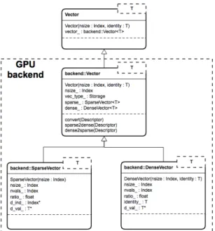
5.6 UML diagram of Vector interface . . . 36

5.7 BFS performance comparison . . . 38

6.1 Aspect ratio vs. performance . . . 42

6.2 SpMV and SpMM load balance . . . 43

6.3 SpMM tiling scheme . . . 44

6.4 Aspect ratio vs. performance (this work) . . . 48

6.5 SpMM performance comparison (selected) . . . 48

6.6 SpMM performance comparison (all) . . . 49

7.1 Decomposition of key GraphBLAS operations . . . 56

7.2 BFS running example . . . 57

7.3 Comparison of SpMV and SpMSpV. . . 61

7.4 Where this work on direction-optimization fits in literature. . . 63

7.5 Comparison with and without fused mask. . . 68

7.6 Graph algorithms using GraphBLAS . . . 71

7.7 Performance comparison for GraphBLAST. . . 76

7.8 Hourglass design of GraphBLAST. . . 78

8.1 Scalability . . . 80

L

T

4.1 BFS performance comparison . . . 16

4.2 SpMSpV datasets . . . 18

4.3 Workload distribution of three SpMSpV implementations . . . 19

4.4 Scalability of three SpMSpV implementations . . . 20

5.1 Matrix-vector computational complexity . . . 24

5.2 BFS optimization summary . . . 32

5.3 BFS datasets . . . 37

6.1 ILP in SpMV and SpMM . . . 45

6.2 SpMM datasets . . . 47

7.1 GraphBLAST matrix and vector methods . . . 53

7.2 GraphBLAST operations . . . 54

7.3 GraphBLAST semirings and monoids . . . 55

7.4 GraphBLAST descriptor settings . . . 56

7.5 Applicability of design principles. . . 60

7.6 Matrix-vector complexity and sparsity . . . 62

7.7 Direction-optimization switching criteria . . . 65

7.8 GraphBLAST load-balancing . . . 69

7.9 GraphBLAST datasets . . . 74

7.10 GraphBLAST performance comparison . . . 75

A

Many people have contributed to making graduate career rewarding and enjoyable. First, I’d like to thank my PhD advisors John D. Owens and Aydın Buluc¸. John taught me about GPUs and that the right way to do computer science research is not to be satisfied with getting a good speed-up, but being able to explain why a speed-up exists. Aydin taught me about sparse linear algebra and pointed me to problems I was capable of solving. Chen-Nee Chuah, Zhaojun Bai and Venkatesh Akella formed the rest of my committee. Their insight and helpfulness improved the quality of this thesis.

I will be forever indebted to colleagues during my years at UC Davis. Yangzihao Wang, Yuechao Pan, Leyuan Wang, and Yuduo Wu have been great collaborators in the Gunrock project. Yangzihao taught me a lot about graph processing and shared my excitement in discov-ering commonalities between the vertex-centric and linear algebra-based perspectives. Yuechao provided a deep understanding about optimizing algorithms on the GPU. Saman Ashkiani, Ja-son Mak, Afton Geil, Muhammad Osama, Shari Yuan, Weitang Liu, Vehbi Bayraktar, Kerry Seitz, Collin Riffel, Andy Riffel, Shalini Venkataraman, Ahmed Mahmoud, Muhammad Awad, Yuxin Chen, Zhongyi Lin, and many others have also brightened up my life.

Thank you to all the people at the Department of Electrical and Computer Engineering at UC Davis, who helped me during my studies: Kyle Westbrook, Nancy Davis, Denise Christensen, Renee Kuehnau, Philip Young, Natalie Killeen, Fred Singh, Sacksith Ekkaphanh, and many more. They kept the department running smoothly and were always there for me.

I am thankful of the generosity of ideas and willingness to help amongst the graph research community. Marcin Zalewski and Peter Zhang taught me much about writing beautiful code, especially when I was getting started. Scott McMillan continually teaches me new ways of using C++. Tim Mattson and Jos´e Moreira taught me much about how to design interfaces.

Finally, I am also grateful for my family’s support. It was with the help of Xinyan Xu that I was able to accomplish this. Her constant love and support make all this worthwhile.

Chapter 1

Introduction

Graphs are a representation that naturally emerges when solving problems in domains including bioinformatics [32], social network analysis [22], molecular synthesis [39], route planning [28]. Problem sizes can be number in over a billion vertices, so parallelization has become a must.

The past two decades has seen the rise of parallel processors to a commodity product—both general-purpose processors in the form of graphic processor units (GPUs), as well as domain-specific processors such as tensor processor units (TPUs) and the graph processors developed under the DARPA SDH (Software Defined Hardware) program. Research into developing par-allel hardware has succeeded in speeding up graph algorithms [61,67]. However, the improve-ment in graph performance has come at the cost of a more challenging programming model. The result has been a mismatch between the high-level languages that users and graph algo-rithm designers would prefer to program in (e.g. Python) and the programming language for parallel hardware (e.g. C++, CUDA, OpenMP, MPI).

To address this mismatch, many initiatives including NVIDIA’s RAPIDS effort [59] have been launched in order to provide an open-source Python-based ecosystem for data science and graphs on GPUs. One such initiative, GraphBLAS is an attractive open standard [18] that has been released for graph frameworks. It promises standard building blocks for graph algorithms in the language of linear algebra. This is exciting, because such a standard attempts to solve the following problems:

Figure 1.1: Mismatch between existing frameworks targeting high-level languages and hard-ware accelerators

1.1

Problem Statement

What is the right set of primitives for expressing graph algorithms? We will define therightset of primitives as one that fulfills the following goals:

1. Performance portability: Graph algorithm does not need modification to have high per-formance across hardware

2. Concise expression: Graph algorithms can be expressed in few lines of code 3. High-performance: Graph algorithms achieve state-of-the-art performance 4. Scalability: Framework is effective at small-scale and exascale

Firstly, the application code ought to require little to no change when targeting different backends. That is to say, the same application code ought to work just as well for single-threaded CPU as for GPU. Secondly, their application code ought to be concise. Thirdly, the graph primitives ought to have high-performance meeting that of “hardwired” code written in a low-level language targeting a particular hardware. Finally, graph algorithms written using the framework should be effective across a wide range of problem scales.

Goal 1 (performance portability) is central to the GraphBLAS philosophy, and it has made inroads in this regard with several implementations already being developed using this common interface [25, 53, 73]. Regarding Goal 2 (concise expression), GraphBLAS encourages users to think in a vectorized manner, which yields an order-of-magnitude reduction in SLOC as evidenced by Table 7.11. Before Goal 4 (scalability) can be achieved, Goal 3high-performance

on the small scale must first be demonstrated.

However, GraphBLAS has lacked high-performance implementations for GPUs. The Graph-BLAS Template Library [73] is a GraphBLAS-inspired GPU graph framework. The architec-ture of GBTL is C++ based and maintains a separation of concerns between a top-level interface defined by the GraphBLAS C API specification and the low-level backend. However, since it was intended as a proof-of-concept in programming language research, it is an order of magni-tude slower than state-of-the-art graph frameworks on the GPU in terms of performance.

We identify several reasons graph frameworks arechallengingto implement on the GPU:

Generalizability of optimization While many graph algorithms share similarities, the opti-mizations found in high-performance graph frameworks often seem ad hoc and difficult to reconcile with the goal of a clean and simple interface. What are the optimizations

most deserving of attention when designing a high-performance graph framework on the GPU?

Load imbalance Graph problems have irregular memory access pattern that makes it hard to extract parallelism from the data. On parallel systems such as GPUs, this is further com-plicated by the challenge of balancing work amongst parallel compute units. How should this problem ofload-balancingbe addressed?

Low compute-to-memory access ratio Graph problems emphasizes making multiple mem-ory accesses on the unstructured data instead of doing a lot of computations. Therefore, graph problems are often memory-bound rather than compute-bound. What can be done to reduce thenumber of memory accesses?

In other words, we are interested in answering the following question: What are the de-sign principles required to build a GPU implementation based in linear algebra that matches the state-of-the-art graph frameworks in performance? Towards that end, we have designed Graph-BLAST1: the first high-performance implementation of GraphBLAS for the GPU (graphics processing unit). Our implementation is for single GPU, but given the similarity between the GraphBLAS interface we are adhering to and the CombBLAS interface [15], which is a graph framework for distributed CPU, we are confident the design we propose here will allow us to extend it to a distributed implementation with future work.

In order to perform a comprehensive evaluation of our system, we need to compare our framework against the state-of-the-art graph frameworks on the CPU and GPU, and hard-wired GPU implementations, which are problem-specific GPU code that someone has hand-tuned for performance. The state-of-the-art graph frameworks we will be comparing against are Ligra [61] for CPU and Gunrock [67] for the GPU, which we will describe in detail in Section 3.2. The hardwired implementations will be Enterprise (BFS) [47], delta-stepping SSSP [24], pull-based PR [43], and bitmap-based triangle counting [14]. The array of graph algorithms we will be evaluating our system on are:

• Breadth-first-search (BFS)

• Single-source shortest-path (SSSP) • PageRank (PR)

• Triangle counting (TC)

A description of these algorithms can be found in Section 7.5. We decided on these four applications, because based on a thorough literature survey by Beamer [9] they are considered the most common four applications across a variety of graph frameworks. Furthermore, they stress different facets of our framework. BFS and SSSP test how well we exploitinput sparsity, PR tests sparse matrix-dense vector (SpMV) performance, and TC tests how well we exploit

output sparsity.

Aside from these four algorithms, we have published elsewhere four algorithms built using our framework: Graph Projections, Seeded Graph Matching and Local Graph Clustering are applications built for the DARPA HIVE program [58], which is aimed at designing new graph processing hardware so our implementation on existing GPU hardware serves as a measure of goodness; Graph Coloring is a work where we compare our framework against Gunrock and hardwired implementations [57].

1

1.2

Thesis Organization

The rest of the thesis will be organized as follows: Chapter 2 gives background information on modern GPU architecture. Chapter 3 presents a survey of large-scale graph frameworks. Chap-ter 4 presents my work on exploitinginput sparsityusing column-based matrix multiplication to do breadth-first-search. Chapter 5 describes my work on exploitingoutput sparsityusing row-based masked matrix multiplication and direction-optimized traversal to do breadth-first-search. Chapter 6 details my work on accelerating sparse matrix-dense matrix multiplication (SpMM). Chapter 7 leverages previous chapters to explain the design principles behind the architecture of GraphBLAST. Finally, Chapter 8 reviews future work that could be done in this area and the remaining research challenges to be solved.

Chapter 2

Background & Preliminaries

This section gives some background information on modern GPU architecture, sparse matrix formats, breadth-first-search, direction-optimized breadth-first-search, and introduces the dual-ity between graph traversal and sparse matrix-vector multiplication that forms a cornerstone to our work.

2.1

GPUs

Modern GPUs are throughput-oriented manycore processors that rely on large-scale multi-threading to attain high computational throughput and hide memory access time. The latest generation of NVIDIA GPUs have up to 80 streaming multiprocessors (SMs), each with up to hundreds of arithmetic logic units (ALUs). GPU programs are calledkernels, which run a large number of threads in parallel in a single-program, multiple-data (SPMD) fashion.

The underlying hardware runs an instruction on each SM on each clock cycle on a warp of 32 threads in lockstep. The largest parallel unit that can be synchronized within a GPU kernel is called a cooperative thread array (CTA), which is composed of warps. For problems that require irregular data access, a successful GPU implementation needs to (1) ensure coalesced memory access to external memory and efficiently use the memory hierarchy, (2) minimize thread divergence within a warp, and (3) maintain high occupancy, which is a measure of how many threads are available to run on the implementation on the GPU.

CPUs use branch prediction, speculative fetching, and large caches tominimizelatency. By contrast, GPUs are throughput-oriented processors, instead relying on thread-level parallelism (TLP) tohidestalls. This means that for running certain irregular computations such as SpMV and SpMM, the bottleneck can be how long a multiply instruction immediately following a memory access must wait. While traditional analyses such as the roofline model [68] focus on compute-bound and memory-bound bottlenecks, we note GPU algorithms can also be latency-bound, which is when the GPU’s parallelism is insufficient to hide the instruction latency.

2.2

Sparse Matrix Formats

Anm×nmatrix is often calledsparseif its number of nonzeroesnnz is small enough compared to O(mn) such that it makes sense to take advantage of sparsity. The most straightforward

sparse matrix format is coordinate (COO) format. This format stores every nonzero as a triple

(i, j,Aij). However, this format requires3nnz memory for storage.

The compressed sparse row (CSR) format stores only the column indices and values of nonzeroes within a row. The start and end of each row is then stored in terms of the column indices and value in arow offsets(or row pointers) array. Hence, CSR only requiresm+ 2nnz

memory for storage.

Similarly to sparse matrix-dense vector multiplication (SpMV), a desire to achieve good performance on SpMM has inspired innovation in matrix storage formatting [2, 56]. These custom formats and encodings take advantage of the matrix structure and underlying machine architecture. Even only counting GPU processors, there exist more than sixty specialized SpMV algorithms and sparse matrix formats [31].

The vendor-shipped library cuSPARSE library provides two functionscsrmmandcsrmm2

for SpMM on CSR-format input matrices [54]. The former expects a column-major input dense matrix and generates column-major output, while the latter expects row-major input and gen-erates column-major output. Among many efforts to define and characterize alternate matrix formats for SpMM are a variant of ELLPACK called ELLPACK-R [56] and a variant of Sliced ELLPACK called SELL-P [2]. However, there is a real cost to deviating from the standard CSR encoding. Firstly, the larger framework will need to convert from CSR to another format to run SpMM and convert back. This process may take longer than the SpMM operation itself. Secondly, the larger framework will need to reserve valuable memory to store multiple copies of the same matrix—one in CSR format, another in the format used for SpMM.

Ortega explores doing SpMM on a specialized matrix storage format, which is a variant on ELLPACK called ELLPACK-R [56]. Along with the usual two vectors that keep the nonzero index and value of standard ELLPACK, the -R variant keeps an additional vector that keeps the nonzero length of each row. Their insight is that by keeping the array in row-major format, they are able to obtain ILP for each thread through loop unrolling.

Anzt, Tomov and Dongarra use another matrix storage format that is a variant of Sliced ELLPACK called SELL-P to compute SpMM [2]. Their insight is that by forming row blocks, and padding (“P” stands for “padding”) them with the number of threads assigned to each row, memory savings can be had over standard ELLPACK. At the same time, most of the advantages of ELLPACK over CSR are maintained.

2.3

Breadth-first-search

A common problem we are trying to solve is a breadth-first search on an unweighted directed or undirected graphG= (V, E). V is the set of vertices ofG, andE is the set of all ordered pairs

(u, v), withu, v ∈V such thatuandv are connected by an edge inG. A graph is undirected if for allv, u ∈ V : (v, u) ∈ E ⇐⇒ (u, v) ∈ E. Otherwise, it is directed. For directed graphs, a vertexu is the child of another vertex v if (v, u) ∈ E and the parent of another vertexv if

(u, v)∈E.

Given a source vertexs∈V, a BFS is a full exploration of graphGthat produces a spanning tree of the graph, containing all the edges that can be reached froms, and the shortest path from

sto each one of them. We define the depth of a vertex as the number of hops it takes to reach this vertex from the root in the spanning tree. The visit proceeds in steps, examining one BFS level

at a time. It uses three sets of vertices to keep track of the state of the visit:frontiercontains the vertices that are being explored at the current depth,nextthe vertices that can be reached from

frontier, andvisitedthe vertices reached so far.

Algorithm 1Sequential breadth-first-search (BFS).

1: procedureSEQUENTIALBFS(vertices, graph, source)

2: frontier← {source}

3: next← {}

4: visited← {-1, -1, ..., -1}

5: depth←0

6: whilefrontier6={}do

7: visited[i]←depth∀is.t. frontier[i]= 0

8: forv ∈frontierdo 9: forn∈neighbors[v]do 10: ifvisited[n] =-1then 11: next←next∪ {n} 12: end if 13: end for 14: end for 15: frontier←next 16: next← {} 17: depth←depth + 1 18: end while 19: returnvisited 20: end procedure

2.4

Direction-optimized Breadth-first-search

Push is the standard textbook way of thinking about BFS. At the start of each push step, each vertex in thefrontierlooks for its children and adds them to the nextset if they have not been visited before. Once all children of the current frontier have been found, the discovered children are added to the visited array with the current depth, the depth is incremented, and thenextset becomes thefrontierof the next BFS step.

Pull is an alternative algorithmic formulation of BFS, yielding the same results but comput-ing thenext set in a different way. At the start of each pull step, each vertex in theunvisited

set of vertices looks for its parents. If at least one parent is part of thefrontier, we include the vertex in thenextset.

Because either push or pull is a valid option to compute each step, we can achieve better overall BFS performance if we make the optimal algorithmic choice at each step. This is the key idea behind direction-optimized breadth-first-search (DOBFS), also known as push-pull BFS [10]. Push-pull can also be used for other traversal-based algorithms [13, 61]. DOBFS implementations use a heuristic function after each step to determine whether push or pull will be more efficient on the next step.

Algorithm 2Direction-optimized BFS.

1: procedureDIRECTIONOPTIMIZEDBFS(vertices, graph, source)

2: frontier← {source}

3: next← {}

4: visited← {-1, -1, ..., -1}

5: depth←0

6: whilefrontier6={}do

7: visited[i]←depth∀is.t. frontier[i] = 0

8: direction←COMPUTEDIRECTION() 9: ifdirection=PUSHthen

10: PUSHSTEP(vertices, graph, frontier, next, visited)

11: else

12: PULLSTEP(vertices, graph, frontier, next, visited)

13: end if 14: frontier←next 15: next← {} 16: depth←depth + 1 17: end while 18: returnvisited 19: end procedure

Algorithm 3Sequential push.

1: procedurePUSHSTEP(vertices, graph, frontier, next, visited) 2: forv ∈frontierdo 3: forn∈children[v]do 4: ifvisited[n]=-1then 5: next←next∪ {n} 6: end if 7: end for 8: end for 9: end procedure

Algorithm 4Sequential pull.

1: procedurePULLSTEP(vertices, graph, frontier, next, visited)

2: forv ∈verticesdo 3: ifvisited[n]=-1then 4: forn∈parents[v]do 5: ifn ∈frontierthen 6: next←next∪ {v} 7: break 8: end if 9: end for 10: end if 11: end for 12: end procedure

2.5

Notation

At this point, we introduce some notation. We follow the MATLAB colon notation where

A(:, i)denotes theith column,A(i,:)denotes theith row, and A(i, j)denotes the element at the(i, j)th position of matrix A. We use.∗to denote the elementwise multiplication operator. For two frontiers u,v, their elementwise multiplication product w = u. ∗ v is defined as

w(i) = u(i)∗v(i)∀i.

For a set of nodesv, we will say the number of outgoing edgesnnz(m+_v)is the sum of the number of outgoing edges of all nodes that belong to this set. Outgoing edges are denoted by a superscript ‘+’, and incoming edges are denoted by a superscript ‘−’. That is, the number of incoming edges for a set of nodesvis

nnz(m−_v) = X

i:v(i)6=0

nnz(AT(i,:)). (2.1)

For matrixA, we will say the number of nonzero elements in it isnnz(A). For a vectorv, we will say the number of elements in the vector isnnz(v).

2.6

Traversal is Matrix-vector Multiplication

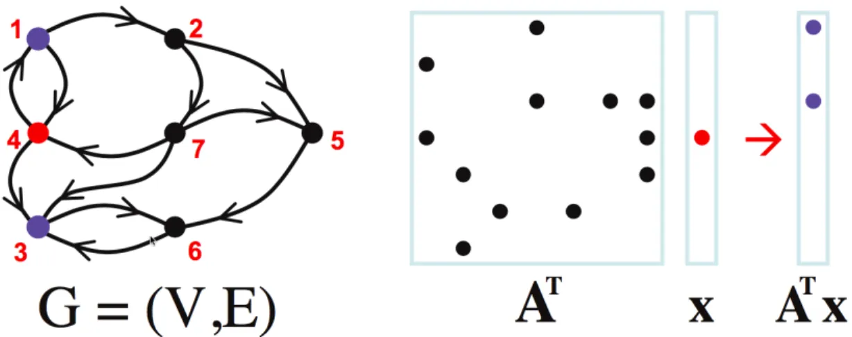
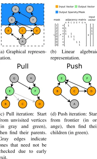
Since the start of graph theory, the duality between graphs and matrices has been established by the popular representation of a graph as an adjacency matrix [44]. After that time, it has become well-known that a vector-matrix multiply in which the matrix represents the adjacency matrix of a graph is equivalent to one iteration of breadth-first-search traversal. This is shown in Figure 2.1.

Figure 2.1: Matrix-graph duality. The adjacency matrixA is the dual of graphG. The current

frontier (set of vertices we want to make a traversal from) is vertex 4. The next frontier is vertices 1 and 3, and is obtained by doing the matrix-vector multiplication. Therefore, the matrix-vector multiply (right) is the dual of the BFS graph traversal (left). Figure is based on Kepner and Gilbert’s book [41].

Chapter 3

Related Work

Large-scale graph frameworks on multi-threaded CPUs, distributed memory CPU systems and massively parallel GPUs fall into three broad categories: vertex-centric, edge-centric and linear algebra-based.

3.1

Literature survey

In this section, we will explain this categorization and the influential graph frameworks from each category.

3.1.1

Vertex-centric

Introduced by Pregel [48], vertex-centric frameworks are based on parallelizing by vertices. Vertex-centric frameworks follow an iterative convergent process (bulk synchronous program-ming model, or BSP) consisting of global synchronization barriers calledsupersteps. The com-putation in Pregel is inspired by distributed CPU programming model of MapReduce [27] and is based on message passing. At the beginning of the algorithm, all vertices are active. At the end of a superstep, the runtime receives the messages from each sending vertex and computes the set of active vertices for the superstep. Computation continues until convergence or a user-defined condition is reached.

Its programming model is good for scalability and fault tolerance. However, standard graph algorithms in most Pregel-like graph processing systems suffer slow convergence on large-diameter graphs and load imbalance on scale-free graphs. Apache Giraph [21] is an open source implementation of Google’s Pregel. It is a popular graph computation engine in the Hadoop ecosystem initially open-sourced by Yahoo!.

3.1.2

Edge-centric (Gather-Apply-Scatter)

First introduced by PowerGraph [34], the edge-centric or Gather-Apply-Scatter (GAS) model is designed to address the slow convergence of vertex-centric models on power law graphs. For the load imbalance problem, it uses vertex-cut to split high-degree vertices into equal degree-sized redundant vertices. This exposes greater parallelism in real-world graphs. It supports both BSP and asynchronous execution. Like Pregel, PowerGraph is a distributed CPU framework. In the linear algebraic model, edge-centric models are analogous to allocating to each processor an

even number of nonzeroes and computing matrix-vector multiply. For flexibility, PowerGraph also offers vertex-centric programming model, which is efficient on non-power law graphs.

3.1.3

Linear algebra-based

Linear algebra-based graph frameworks are pioneered by the Combinatorial BLAS (Comb-BLAS) [15], a distributed me mory CPU-based graph framework. Algebra-based graph frame-works rely on the fact that graph traversal can be described as a matrix-vector product. Comb-BLAS offers a small, but powerful set of linear algebra primitives. Combined with algebraic semirings, this small set of primitives can describe a broad set of graph algorithms. The ad-vantage of CombBLAS is that it is the only framework that can express a 2D partitioning of adjacency matrix, which is helpful in scaling to large-scale graphs.

In the context of bridging the gap between vertex-centric and linear algebra-based frame-works, GraphMat [62] is groundbreaking work. Traditionally, linear algebra-based frameworks have found difficulty gaining adoption, because they rely on users to understand how to express graph algorithms in terms of linear algebra. GraphMat addresses this problem by exposing a vertex-centric interface ot the user, automatically converting such a program to a generalized sparse matrix-vector multiply, and then performing the computation on a linear algebra-based backend.

nvGRAPH [30] is a high-performance GPU graph analytics library developed by NVIDIA. It views graph analytics problems from the perspective of linear algebra and matrix compu-tations [42], and uses semiring matrix-vector multiply operations to present graph algorithms. As of version 10.1, it supports five algorithms: PageRank, single-source shortest-path (SSSP), triangle counting, single-source widest-path, and spectral clustering. SuiteSparse [25] is no-table for being the first GraphBLAS-compliant library. However, it currently only supports single-threaded CPU implementation.

3.2

Previous systems

Two systems that directly inspired our contribution are Gunrock and Ligra.

3.2.1

Gunrock

Gunrock [67] is a state-of-the-art GPU-based graph processing framework. It is notable for be-ing the only high-level GPU-based graph analytics system, with support for both vertex-centric and edge-centric operations, as well as fine-grained runtime load balancing strategies, without requiring any preprocessing of input datasets. However, since Gunrock has many performance optimizations, Gunrock provides much flexibility in terms of choosing kernel variants the user wants to use. In our work, we aim to extract the performance Gunrock optimizations provide while delegating much of kernel selection work to the backend. This allows us to adhere to GraphBLAS’s compact and easy to use user interface, while maintaining state-of-the-art per-formance.

3.2.2

Ligra

Ligra [61] is a CPU-based graph processing framework for shared memory. Its lightweight implementation is targeted at shared memory architectures and uses CilkPlus for its

multi-threading implementation. It is notable for being the first graph processing framework to generalize Beamer, Asanovi´c and Patterson’s direction-optimized BFS [10] to many graph traversal-based algorithms. However, Ligra does not support multi-source graph traversals. In our framework, multi-source graph traversals find natural expression as BLAS 3 operations (matrix-matrix multiplications).

Chapter 4

Fast Sparse Matrix and Sparse Vector

Multiplication Algorithm on the GPU

The motivating question for our work is given that the frontier vector (representing the set of vertices we would like to perform graph traversal from) is typically sparse, can we perform a sparse matrix-vector multiplication more efficiently than having to traverse the entire sparse matrix?

Before our work, there was research on sparse matrix-sparse vector in the CPU world [16,

33] and by the traversal matrix-vector duality discussed in Section 2.6 it was typical for tra-ditional, graph-centric frameworks on the GPU. However, there were no sparse matrix-sparse vector implementations for the GPU, so we are the first to introduce this primitive to the GPU where the primitive is a cornerstone for any high-performance graph framework.

In this work, we show that a new primitive called sparse matrix-sparse vector multiplication (SpMSpV) is required in order to do graph algorithms efficiently. It performs favourably com-pared to sparse-matrix-dense vector multiplication (SpMV). Our contributions in this work are as follows:

1. We implement a promising algorithm for doing fast and efficient SpMSpV on the GPU. 2. We examine the various optimization strategies to solve thek-way merging problem that

makes SpMSpV hard to implement on the GPU efficiently.

3. We provide a detailed experimental evaluation of the various strategies by comparing with SpMV and two state-of-the-art GPU implementations of breadth-first-search (BFS).

4.1

Algorithms and Analysis

Algorithm 5 gives the high-level pseudocode of our parallel algorithm. The sparse vectorxis passed into the MULTIPLYBFS in dense representation. The STREAMCOMPACT consisting of

1_{This chapter substantially appeared as “Fast Sparse Matrix and Sparse Vector Multiplication Algorithm on the} GPU” [70], for which I was responsible for most of the research and writing.

Algorithm 5SpMSpV multiplication algorithm for BFS.

Input: Sparse matrixG, sparse vectorx(in dense representation)

Output: Sparse vectorw=GT _×x

1: procedureMULTIPLYBFS(G,x)

2: STREAMCOMPACT(x) 3: ind⇐GATHER(G,x) 4: SORTKEYS(ind)

5: w⇐SCATTER(ind)

6: end procedure

a scan and scatter is used to put the sparse vector into a sparse representation. The natively-supported scatter operation here is a moving of elements from the original arrayxinto a list of new indices given by scan.

This sparse vector representation can be considered an analogue of the CSR format, with the simplification that since there is only one row, so the column-indices arrayC–which simplifies to the array with two elements[0, m]–will be replaced by a single variable,m.

Since the vector is sparse, we use something akin to outer product rather than SpMV’s inner product. We do a linear combination on the rows of the matrixG. Even though the product we get isGT ×x, we do not need to do a costly transposition in both memory storage and access since that is exactly the product we need for BFS. This way, we are only performing multiplica-tion when we know for certain the resulting product is nonzero. This is the fundamental reason why SpMSpV is more work-efficient than SpMV.

To get the rows of G, we do a gather operation on the rows we are interested in and con-catenate them into one array. The use of this single array is our attempt of solving the multiway merging problem in parallel, which is mentioned in Buluc¸ and Madduri [16]. By concatenating into a single array, we are able to avoid atomic operations, which are known to be costly.

Going into more detail about this gather operation, we use the sparse vector x to get an index into graphG. (1) Then for alli ∈ indwe gather from the graph’s column-indices array obtaining two indicesC[i]andC[i+ 1]. These two indices give us the beginning and end of row

iwe are interested in. (2) Next, for allh ∈ [C[i], C[i+ 1])we gather elements of row-offsets arrayR[h]and call this setind_i. The first two gather operations are shown as a single gather in Line 3 of Algorithm 5 and Algorithm 6.

In the case of Algorithm 6, we perform a third gather. This is to obtain the corresponding valueGVal[h]of node indexR[h]over the same interval[C[i], C[i+ 1]). We are now faced with the problem of doing ak-way merge of different-sizedindi withinind. We tried three different

approaches: 1. No sort. 2. Merge sort. 3. Radix sort.

We first try no sorting. Since the array is unsorted, adjacent threads do not write adjacent values; we instead scatter outputs to their memory destinations. The result is uncoalesced writes

Runtime (ms) Dataset Description

Dataset SpMSpV Gunrock b40c Vertices Edges Max Degree Diameter

ak2010 1.686 0.932 0.104 45K 25K 199 15 belgium osm 63.937 13.053 1.277 1.4M 1.5M 9 630 coAuthorsDBLP 4.530 2.829 0.452 0.30M 0.98M 260 36 delaunay 13 1.085 0.820 0.117 8.2K 25K 10 142 delaunay 21 11.511 2.207 0.259 2.1M 6.3M 17 230 soc-LiveJournal1 73.722 33.953 21.117 4.8M 68.9M 20333 16 kron g500-log21 70.935 15.194 23.423 2.1M 90M 131503 6

Table 4.1: Dataset descriptions and performance comparison of our SpMSpV implementation against two state-of-the-art BFS implementations on a single GPU for seven datasets.

into GPU memory, with a resulting loss of memory bandwidth. Davidson et al. [24] use a similar strategy when they remove duplicates in parallel in their single-source shortest-path (SSSP) algorithm.

Since we are skipping the sorting, we avoid the logarithmic time factor of merge sort men-tioned by Buluc¸ et al. [16]. We scatter 1’s into a dense array using the concatenated array value as the index. This approach trades off less work in sorting for lower bandwidth from uncoalesced memory writes.

Algorithm 6Generalized SpMSpV multiplication algorithm.

Input: Sparse matrixG, sparse vectorx(in dense representation), operator⊕, operator⊗.

Output: Sparse vectorw=GT _×x.

1: procedureMULTIPLY(G,x,⊕,⊗) 2: STREAMCOMPACT(x)

3: ind⇐GATHER(G,x)

4: GVal⇐GATHER(G,ind) 5: SORTPAIRS(ind,GVal)

6: for eachj ∈indin parallel do 7: flag[j]⇐1

8: val[j]⇐GVal[j]⊗x[j]

9: ifind[j] =ind[j−1]then 10: flag[j]⇐0

11: end if

12: end for

13: wVal⇐SEGREDUCE(val,flag,⊕) 14: w⇐SCATTER(wVal,ind)

15: end procedure

To increase our achieved memory bandwidth, we could perform the k-way merge by sort-ing. We first try a merge sort, which doesO(flogf)work, wheref is the size of the frontier. Though this asymptotic complexity—which isO(mlogm)in the worst case—sounds bad

com-pared to theO(m)work of SpMV, it is actually much faster in practice due to the nature of BFS on typical graph topologies, which rarely visits a large fraction of the graph’s vertices on a single iteration.

We also try radix sort, which hasO(kf) work, wherek is the length of the largest key in binary. We expect merge sort to be compute-bound; no-sorting to be memory-bound; and radix sort somewhere between the two. We investigate which is more efficient in practice.

Algorithm 6 is a generalized case of matrix multiplication parameterized by the two opera-tions (⊕,⊗). If we set those two operations to (∪,∩), we obtain Algorithm 5. For low-diameter, power-law graphs, it is well-known that there are a few iterations whenf becomes dense and these are the iterations that dominate the overall running time. For the remainder of BFS itera-tions, it is wasteful to use a dense vector.

We will investigate whether this crossing point is a fixed number independent of the total number of vertices or edges in the graph or whether it is determined by the percent of descen-dants f out of the total number of edges. The former would indicate a limit to SpMSpV’s scalability since it would only be interesting for a small number of cases, while the latter would demonstrate that SpMSpV could outperform SpMV for BFS calculations on graphs of any scale provided they have a topology similar to those we perform our scalability tests.

4.2

Experiments and Results

We ran all experiments in this paper on a Linux workstation with 2× 3.50 GHz Intel 4-core E5-2637 v2 Xeon CPUs, 528 GB of main memory, and an NVIDIA K40c GPU with 12 GB on-board memory. The GPU programs were compiled with NVIDIA’s nvcc compiler (ver-sion 6.5.12). The C code was compiled using gcc 4.6.4. All results ignore transfer time (from disk-to-memory and CPU-to-GPU). The Gunrock code was executed using the command-line configuration --src=0 --directed --idempotence --alpha=6. The merge sort is from the Modern GPU library [8]. The radix sort is from the CUB library [50].

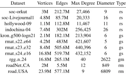
The datasets used in our experiments are shown in Table 4.1. The graph topology of the datasets varies from small-degree large-diameter to scale-free. The soc-LiveJournal1 (soc) and kron g500-logn21 (kron) datasets are two scale-free graphs with diameter less than 20 and unevenly distributed node degree. The belgium-osm dataset has a large diameter with small and evenly distributed node degree.

Performance summary Looking at the comparison with two state-of-the-art BFS implemen-tations, SpMSpV is between 2–4x slower. Nevertheless, this shows our implementation is a reasonable implementation, with runtime results in the same ballpark. With some Gunrock optimizations (that are not implemented in our system) turned off, the results are even closer.

One such BFS-specific optimization is direction-optimized traversal (discussed in detail in Chapter 5). This optimization is known to be effective when the frontier includes a substantial fraction of the total vertices [10]. Another reason may be kernel fusion [52]: b40c is careful to take advantage of producer-consumer locality by merging kernels together whenever possible. This way, costly reads and writes to and from global memory are minimized. Apart from that, both b40c and Gunrock use load-balancing workload mapping strategies during the neighbor list expanding phase of the traversal. Compared to b40c, Gunrock implements the direction-optimized traversal and more graph algorithms than BFS.

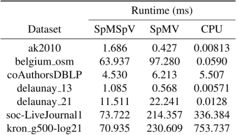
Runtime (ms) Dataset SpMSpV SpMV CPU ak2010 1.686 0.427 0.00813 belgium osm 63.937 97.280 0.0590 coAuthorsDBLP 4.530 6.213 5.507 delaunay 13 1.085 0.568 0.00571 delaunay 21 11.511 22.241 0.0128 soc-LiveJournal1 73.722 214.357 336.384 kron g500-log21 70.935 230.609 753.737

Table 4.2: Performance comparison of our SpMSpV with SpMV for computing BFS on a single GPU for seven datasets.

Comparison with SpMV Table 2 compares SpMSpV’s performance against SpMV. SpM-SpV is 1.26x faster than SpMV at performing BFS on average. The primary reason is simply that SpMV does more work, performing multiplications on zeroes in the dense vector. The speed-up of SpMSpV is most prominent on scale-free graphs “soc” and “kron” where it is 2.9x and 3.3x faster. This is likely because on larger graphs, the work-efficiency of SpMSpV becomes prominent.

Such a conclusion is supported by the road network graph “belgium”. It has a large number of edges, but both the average and max degrees are low while the diameter is high. In spite of being a graph of similar size to “delaunay 21”, since not many edges need traversal every itera-tion there is not much difference in work-efficiency between the SpMSpV and SpMV. Perhaps superior load-balancing in the SpMV kernel is the difference maker. In the same vein, it can be seen that on the two smallest graphs “ak2010” and “delaunay 13”, SpMV is 3.9x and 1.9x faster.

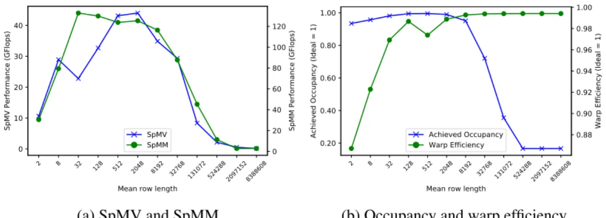
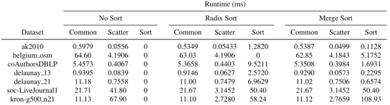
Figure 4.1 shows the impact of coalesced memory access on the scatter operation. With-out sorting, scatter write takes up a majority of computation time for large datasets, but be-comes neglible if prior sorting has been done. The only exception is for the road network graph belgium-osm, which has a high diameter and low node degree. This could be because the neighbor list is small every time and everything in the neighbor list is kept in sorted order, so there is little gained from performing a costly sort operation. The unnormalized data is given in Table 4.3.

Some parts of our SpMSpV implementations are common to all three of our approaches. We see some variance in this common code across our tests. Some of this variance is due to the method by which the execution times were measured, which was using the cudaEventRecord API. The rest of the variance is due to natural run-to-run variance of the GPU. This is why when possible, the runtimes taken were the average of ten iterations.

Figure 4.2 shows the runtime of BFS on a scale-free network (“kron”) plotted against the number of edges traversed. SpMSpV implemented using radix sort and merge sort scale lin-early, while SpMV (shown in Table 4.4 and SpMSpV with no sorting scale superlinearly. For a small number of edges, it is faster to do SpMSpV without sorting. Since SpMSpV seems to perform better than SpMV on bigger datasets, it seems that the answer as to whether the

ak2010 _{belgium_osm coAuthorDBLP delaunay_n13 delaunay_n21 Soc-LiveJournal1kron-g500_n21} 0.0 0.2 0.4 0.6 0.8 1.0 1.2 Common Scatter Sort No Sort Radix Sort Merge Sort

Figure 4.1: Workload distribution of three SpMSpV implementations. Shown are no sorting, radix sort and merge sort for the datasets listed in Table 1.

0 10 20 30 40 50 60 70 80 90

Edges Traversed (millions)

0 20 40 60 80 100 120 140 Runtime (ms) No Sorting Radix Sort Merge Sort

Figure 4.2: Performance comparison of three SpMSpV implementations on six differently-sized synthetically-generated Kronecker graphs with similar scale-free structure. The raw data used to generate this figure is given in Table 4.4. Each point represents a BFS kernel launch from a different node. Ten different starting nodes were used in this experiment.

Runtime (ms)

No Sort Radix Sort Merge Sort

Dataset Common Scatter Sort Common Scatter Sort Common Scatter Sort

ak2010 0.5979 0.0556 0 0.5349 0.05433 1.2820 0.5387 0.0499 0.1128 belgium osm 64.60 4.1906 0 63.03 4.1906 0 62.85 4.1843 5.1752 coAuthorsDBLP 5.4573 0.4067 0 5.3658 0.4403 9.5211 5.3508 0.3984 1.6931 delaunay 13 0.9395 0.0839 0 0.9146 0.0627 2.5720 0.9290 0.0573 0.2295 delaunay 21 11.18 0.7558 0 11.00 0.7479 6.9629 11.02 0.7506 0.6574 soc-LiveJournal1 21.71 41.80 0 21.67 3.1452 50.40 21.67 3.1452 50.40 kron-g500 n21 11.13 67.90 0 11.10 2.7280 58.24 11.12 2.7659 108.93

Table 4.3: Workload distribution of three SpMSpV implementations showing runtime (ms) on a single GPU for seven datasets. Common refers to time spent running the kernels common to all three implementations.

crossing point beyond which SpMV becomes more efficient than SpMSpV is governed not by a fixed frontier size, but rather as a function of both frontier size and the total number of edges as well. This indicates that SpMSpV is competitive with SpMV not just on datasets of limited size, but large datasets as well.

To explain the superlinear scaling, we offer a few likely explanations. One is that congestion degrades memory access latency [7]. As Figure 4.1 shows, the scatter writes are the difference between no sort and sort. One phenomenon that was observed was that if only a few iterations of merge and radix sort were performed, there would be no effect on scatter time and thereby increase the total execution time. Perhaps if a sorting algorithm that divides the array in a

man-Runtime (ms) Edge rate (MTEPS)

Dataset No Sorting SpMV Radix Sort Merge Sort No Sort SpMV Radix Sort Merge Sort

kron-16 1.37 2.21 4.74 3.81 1401.9 868.3 405.07 503.9 kron-17 1.71 4.02 5.81 5.35 1923.5 819.6 567.3 615.2 kron-18 2.85 7.70 9.79 11.37 2764.8 1022.8 804.7 692.4 kron-19 6.79 19.94 16.85 22.31 2372.0 807.9 955.8 721.8 kron-20 21.08 75.97 29.25 43.13 1469.0 407.7 1058.7 718.2 kron-21 68.09 259.86 64.23 105.92 1087.7 285.0 1153.0 699.2

Table 4.4: Scalability of three SpMSpV implementations and one SpMV implementation (run-time and edges traversed per second) on a single GPU on six differently-sized synthetically-generated Kronecker graphs with similar scale-free structure. Radix sort and merge sort scale linearly; no sorting and SpMV show non-ideal scaling.

ner like quick sort or bucket sort were used, more coalesced memory access could be attained at the cost of additional computation.

Another way to express this idea is that there is an optimal compute to memory access ratio specific for each particular GPU hardware model. It is possible that the no sort implementation reached peak compute to memory access for dataset “kron g500-logn18”, but for larger datasets memory access grew faster than the amount of gather operations, so memory accesses were becoming degraded by congestion. The sorting methods may be closer to the compute-limited side of the compute to memory access peak, so the increased memory accesses are bringing them closer to peak performance.

4.3

Conclusion

In this paper we implement a promising algorithm for computing sparse matrix sparse vector multiplication on the GPU. Our results using SpMSpV show considerable performance im-provement for BFS over the traditional SpMV method on power-law graphs. We also show that our implementation of SpMSpV is flexible and can be used as a building block for a linear algebra-based framework for implementing other graph algorithms.

An open research question now is how to optimize the compute to memory access ratio to maintain linear scaling. We showed merge sort and radix sort are good options, but it is possible a partial quick sort or a hybrid k-way merge algorithm such as the one presented by Leischner [46] can be used to obtain a better compute to memory access ratio, and better performance.

The SpMSpV algorithm used in this paper is generalizable to other graph algorithms through Algorithm 6. This algorithm is still being implemented in CUDA. By setting(⊕,⊗)to(+,×), one performs standard matrix multiplication. A direction may be using SpMSpV as a building block for sparse matrix sparse matrix multiplication. Buluc¸ and Gilbert’s work in simulating parallel SpGEMM sequentially using SpMSpV has been promising [19]. Similarly, by setting

(⊕,⊗)to(min,+), one performs single-source shortest path (SSSP).

In this chapter, we saw that direction-optimized BFS is one reason Gunrock attained such high performance. In the next chapter, we address the problem of expressing direction-optimized BFS using linear algebra.

Chapter 5

Implementing Push-Pull Efficiently in

GraphBLAS

In the previous chapter, we saw that direction-optimized BFS was a reason why our system per-formed worse than Gunrock. In this chapter, we solve the problem of how to express direction-optimized BFS using linear algebra.

In order to do so, we needed to factor Beamer’s direction-optimized BFS [10] into 3 sep-arable optimizations, and analyze them independently—both theoretically and empirically—to determine their contribution to the overall speed-up. This allows us to generalize these opti-mizations to other graph algorithms, as well as fit it neatly into a linear algebra-based graph framework. These 3 optimizations are, in increasing order of specificity:

1. Change of direction: Usepushdirection to take advantage of knowledge that the frontier is small, which we terminput sparsity. When the frontier becomes large, go back topull

direction.

2. Masking: Inpulldirection, there is an asymptotic speed-up if we knowa priorithe subset of vertices to be updated, which we termoutput sparsity.

3. Early-exit: Inpull direction, once a single parent has been found, the computation for that undiscovered node ought to exit early from the search.

Previous work by Beamer et al. [11] and Besta et al. [13] have observed that push and pull correspond to column- and row-based matrix-vector multiplication (Opt. 1). However, this knowledge is not exploited in the sole GraphBLAS implementation in existence so far, namely SuiteSparse GraphBLAS [25]. In SuiteSparse GraphBLAS, the BFS executes in only the forward (push) direction.

The key distinction between our work and that of Shun, Besta and Beamer is that while they take advantage of input sparsity using change of direction (Opt. 1), they do not analyze usingoutput sparsity through masking (Opt. 2), which we show theoretically and empirically

1_{This chapter substantially appeared as “Implementing Push-Pull Efficiently in GraphBLAS” [72], for which I} was the first author and responsible for most of the research and writing.

(in Table 5.1 and 5.2 respectively) is critical for high performance. Furthermore, we submit this speed-up extends to all algorithms for which there isa prioriinformation regarding the sparsity pattern of the output such as triangle counting and enumeration [5], adaptive PageRank [40], batched betweenness centrality [17], maximal independent set [18], and convolutional neural networks [20].

Since the input vector can be either sparse or dense, we refrain from referring to this opera-tion as SpMSpV (sparse matrix-sparse vector) or SpMV (sparse matrix-dense vector). Instead, we will refer to it as matvec (short for matrix-vector multiplication and known in GraphBLAS asGrB mxv). Our contributions in this paper are:

1. We provide theoretical and empirical evidence of the asymptotic speed-up from masking, and show it is proportional to the fraction of nonzeroes in the expected output, which we termoutput sparsity.

2. We provide empirical evidence that masking is a key optimization required for BFS to attain state-of-the-art performance on GPUs.

3. We generalize the concept of masking to work on all algorithms where output sparsityis known before computation.

4. We show that direction-optimized BFS can be implemented in GraphBLAS with minimal change to the interface by virtue of an isomorphism between push-pull, and column- and row-based matvec.

5.1

Types of Matvec

The next sections will make a distinction between the different ways the matvecy ←Axcan be computed. We define matvec as the multiplication of a sparse matrix with a vector on the right. This definition allows us to classify algorithms as row-based and column-based without ambiguity. We draw a distinction between SpMV (sparse matrix-dense vector multiplication) and SpMSpV (sparse matrix-sparse vector multiplication). Our analysis differs from previous work that focuses on the former, while we concentrate on the latter. Our novelty also comes from analysis of their masked variants, which is a mathematical formalism for taking advantage ofoutput sparsityand to the best of our knowledge does not exist in the literature.

As mentioned in the introduction, we will henceforth refer to SpMV as row-based matvec, and SpMSpV as column-based matvec. We feel this is justified because although it is possible to implement SpMV in a column-based way and SpMSpV in a row-based way, it is generally more efficient to implement SpMV by iterating over rows of the matrix [65] and SpMSpV by fetching columns of the matrix A(:, i) for which x(i) 6= 0 [4]. Here, we are talking about SpMV and SpMSpV without direct dependence on graph traversal. Hence we use the common, untransposed problem descriptiony←Axinstead of that specific to graph traversal case.

5.1.1

Row- and column-based matvec

We wish to understand, from a matrix point of view, which of row- and column-based matvec is more efficient. We quantify efficiency with the random-access memory (RAM) model of computation. Since we assume the input vector must be read in both row- and column-based matvec, we will focus our attention on the number of random memory accesses into matrixA.

Row-based matvec The efficiency of row-based matvec is straightforward. For all rowsi = 0,1, ..., M:

f0(i) = X

j:A(i,j)6=0

A(i, j)×f(j) (5.1)

No matter what the sparsity of f, each row must examine every nonzero, so the number of memory accesses into the matrix required to compute Equation 5.1 is simplyO(nnz(A)).

Column-based matvec However, computing matvec ought to be more efficient if the vector

f is all 0 except for just one element. We define such a situtation as input sparsity. Can we compute a result without touching all elements in the entire matrix? This is the benefit of column-based matvec: if only f(i)is nonzero, then f0 is simply theith column ofA i.e., A(:

, i)×f(i).

f0 = X

i:f(i)6=0

A(:, i)×f(i) (5.2)

Whenf has more than one non-zero element (whennnz(f) > 1), we must accessnnz(f)

columns inA. How do we combine these multiple columns into the final vector? The necessary operation is a multiway merge of A(:, i)f(i) for alli wheref(i) 6= 0. Multiway merge (also known ask-way merge) is the problem of mergingksorted lists together such that the result is sorted [3]. It arises naturally in column-based matvec from the fact that the outgoing edges of a frontier do not form a set due to different nodes trying to claim the same child. Instead, one obtainsnnz(f)lists, and has to solve the problem of merging them together.

According to the literature, multiway merge takesnlogk memory accesses wherek is the number of lists andnis the length of all lists added together. For our problem where we have

k =nnz(f)andn=nnz(m+_f ), so the multiway merge takesO(nnz(m+_f ) lognnz(f)).

Summary The complexity of row-based matvec is a constant; we need to touch every element of the matrix even if we want to multiply by a vector that is all 0’s except for one index. On the other hand, the complexity of column-based matvec scales withnnz(m+_f ). This matches our intuition, as well as the result of previous work [61], that shows column-based matvec should be more efficient whenf is sparse.

5.1.2

Masked matvec

A useful variant of matvec ismasked matvec. The intuition behind masked matvec is that it is a mathematical formalism for taking advantage ofoutput sparsity (i.e., when we know which elements are zero in the output).

More formally, by masked matvec we mean computingf0 = (Af).∗mwhere vectorm∈

RM×1 and .∗ represents the element-wise multiplication operation. This concept of masking

gives us two new definitions for row- and column-based masked matvec. Byrow-based masked matvec, we mean computing for all rowsi= 0,1, ..., M:

f0(i) =

( P

j:A(i,j)6=0A(i, j)×f(j) ifm(i)6= 0

Operation Cost Expected Cost Row- unmasked O(nnz(A)) O(dM)

based masked O(nnz(m−_m)) O(d nnz(m))

Column- unmasked O(nnz(m+_f ) logM) O(d nnz(f) logM)

based masked O(nnz(m+_f ) logM) O(d nnz(f) logM)

Table 5.1: Four sparse matvec variants and their associated cost, measured in terms of number of memory accesses (actual and in expectation) into the sparse matrixArequired.

Similarly forcolumn-based masked matvec:

f0 =m.∗ X

i:f(i)6=0

A(:, i)×f(i) (5.4)

The intuition behind masked matvec is that if more elements are masked out (i.e., m(i) = 0

for many indicesi), then we ought to be doing less work. Looking at the definition above, we no longer need to go through all nonzeroes inA, but merely rowsA(i,:)for whichm(i) 6= 0. Thus as shown in Figure 5.3c wherem = ¬v, the number of memory accesses decreases to

O(nnz(m−_m)).

For column-based masked matvec, the number of memory accesses is that of computing column-based matvec, and doing an elementwise multiply with the mask, so the amount of computation does not decrease compared to the unmasked version. At this time, we do not know of an algorithm for column based matvec that can take advantage of the sparsity ofmand thus reduce the number of memory accesses accordingly.

A summary of the complexity analysis above is shown in Table 5.1. We choose a matrix (‘kron g500-logn21’ from the 10th DIMACS challenge [6]) and perform a microbenchmark to demonstrate the validity of this analysis. We will refer to it as ‘kron’ henceforth. We use the experimental setup described in Section 5.5. We measure the runtime of four variants given above for increasing frontier sizes (for the two column-based matvecs), and increasing unvisited node counts (for the two row-based matvecs):

1. Row-based: increasennz(f), no mask

2. Row-based masked: nnz(f) = M, increasennz(m)

3. Col-based: increasennz(f), no mask

4. Col-based masked: increasennz(f), increase mask at 2₃nnz(f)

Nodes were selected randomly to belong to the frontier and unvisited nodes. Here, we are using frontier sizennz(f)as a proxy fornnz(mf). The number of outgoing edgesnnz(mf)≈

d nnz(f), wheredis the average number of outgoing edges per node. Similarly, we usennz(m)

as a proxy fornnz(mm).

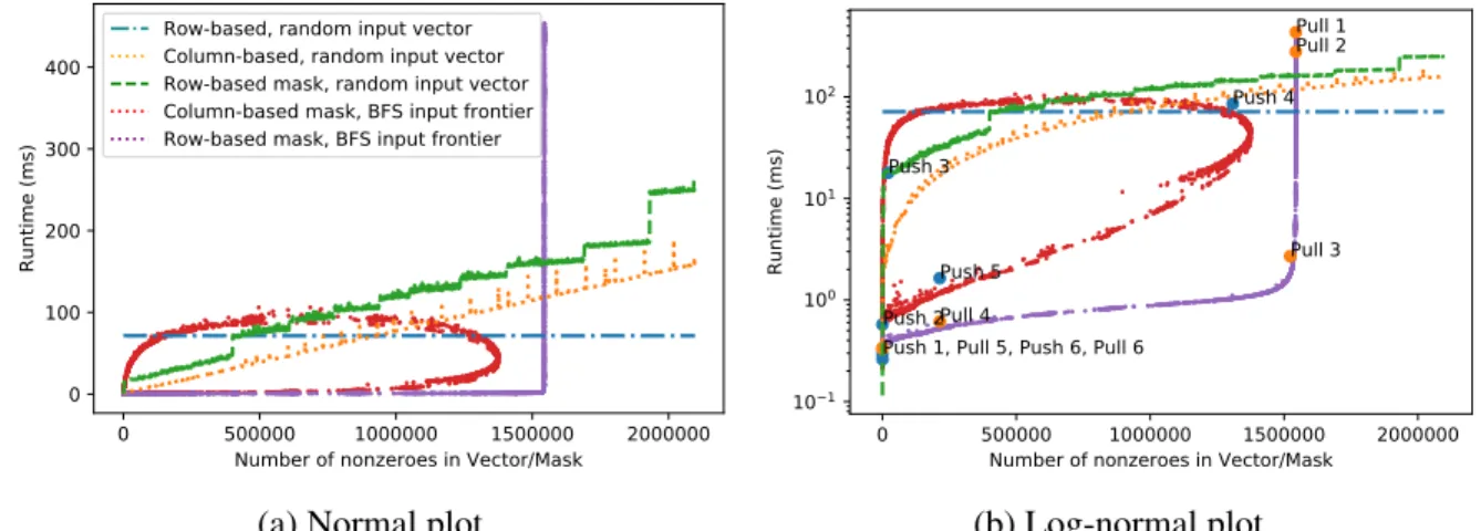
The results are shown in Figure 5.1. They agree with our derivations above. For a given matrix, the row-based matvec’s runtime is independent of a varying frontier size and unvisited

0 500000 1000000 1500000 2000000 Number of nonzeroes in Vector/Mask

0 50 100 150 200 250 Runtime (ms) Row-based

Column-based (mask and no mask) Row-based mask

Figure 5.1: Runtime in milliseconds for row-based and column-based matvec in their masked and unmasked variants for matrix ‘kron’ as a function ofnnz(f)andnnz(m).

node count. The runtime of the column-based matvec and the masked row-based matvec both increase with frontier size and unvisited node count, respectively. For low values of either frontier size or unvisited node count, doing either column-based matvec or masked row-based matvec is more efficient than row-based matvec. For high values of either frontier size or unvisited node count, doing the row-based matvec can be more efficient.

In Section 5.3, we will show that it is by staying in this region (low frontier size and low un-visited node count) through intelligent switching between column-based and row-based masked matvecs is what enables an entire BFS traversal to complete in less time than even a single row-based matvec.

5.1.3

Structural complement

Another useful concept is thestructural complement. Recall the intuition behind masked matvec is that if the mask vectormis 1 at some indexi, then it will allow the result of the computation to be passed through to the outputf0(i). The structural complement operator¬is a user-controlled switch that lets them invert this rule: all the indicesifor whichmwere 1 will now prevent the result of the computation to be passed through to the outputf0(i), while the indices that were 0 will allow the result ot be passed through.

5.1.4

Generalized semirings

One important feature that GraphBLAS provides is that it allows users to express different traversal graph algorithms such as BFS, SSSP (Bellman-Ford), PageRank, maximal indepen-dent set, etc. using matvec and matmul [41]. This way, the user can succinctly express the desired graph algorithm in a way that makes parallelization easy. This is analogous to the key role Level 3 BLAS (Basic Linear Algebra Subroutines) plays in scientific computing; it is much easier to optimize for a set of standard operations than have scientists optimize every applica-tion all the way down to the hardware-level. The mechanism in which they are able to do so is calledgeneralized semirings.

What generalized semirings do is allow the user to replace the standard matrix multipli-cation and addition operation over the real number field with zero-element 0 (_R,×,+,0) by any operation they want over arbitrary field _D with zero-element _I (_D,⊗,⊕,_I). We refer to

the latter asmatvec over semiring(D,⊗,⊕,I). We also have the row-based and column-based

equivalents for all semirings. For example,row-based matvec over semiring(_D,⊗,⊕,_I) is:

f0(i) = n M A(i,j)6=I j=0 A(i, j)⊗f(j)

For row-based masked and column-based masked matvec over semirings, we generalize the element-wise operation to be: _D×_D2 → Dwhere D2 is the set of allowable values of the

mask vectormand_Dis the set of allowable values of the matrixAand vectorf. For example,

row-based masked matvec over semiring(_D,⊗,⊕,_I)and element-wise multiply: _D×_D2 →D

is: f0(i) =m. n M A(i,j)6=I j=0 A(i, j)⊗f(j)

As an example, if the user wants to change from BFS to SSSP, they must specify a change to the semiring from the Boolean semiring({0,1}, OR, AN D,0)to the tropical semiring(_R∪

{∞}, min,+,∞) and removing the masks from the GrB assign and GrB mxv. Then with

this simple change to 2 lines of code, the GraphBLAS application code would support high-performance SSSP code on any hardware backend for which there exists a GraphBLAS imple-mentation.

5.2

Relating Matvec and Push-Pull

In this section, we discuss the connection between masked matvec and the three optimizations inherent to DOBFS. Then, we discuss two closely related optimizations that were not in the initial direction-optimization paper [10] by Beamer, Asanovi´c, and Patterson. In recent work, these authors looked at matvec in their row- and column-based variants for PageRank [11]. They examine three blocking methods (cache, propagation and deterministic propagation) for computing matvec using row- and column-based approaches. Besta et al. also observed the duality between push-pull and row- and column-based matvec in the context of several graph algorithms. They give a theoretical analysis on three parallel random access memory (PRAM) variants for differences between push-pull. We extend their push-pull analysis to include the concept of masking, which is needed to take advantage of output sparsity and express early exit.

5.2.1

Connection with push

To demonstrate the connection with push-pull, we consider the formulation of the problem usingf0 = ATf.∗ ¬v in the specific context of one BFS iteration. In graphical terms, this is visualized as Figure 5.2a. Our current frontier is shown by nodes marked in orange. The visited vectorvindicates the already visited nodesA, B, C, D.

We will first consider the push case as shown in Figure 5.2d. We must examine all edges leaving the current frontier. Doing so, we examine the children ofB, C, D, and combine them using a logical OR. This allows us discover nodesA, E, F. From these 3 nodes, we must filter using the visited vectorvand eliminateAfrom our frontier. This leaves us with the two nodes

(a) Graphical represen-tation.

(b) Linear algebraic representation.

(c) Pull iteration: Start from unvisited vertices (in gray and green), then find their parents. Gray edges indicate ones that need not be checked due to early exit.

(d) Push iteration: Start from frontier (in or-ange), then find their children (in green).

Figure 5.2: Simple example showing BFS traversal from the 3 nodes marked or-ange. There is a one-to-one correspon-dence between the graphical representation of both traversal strategies and their respective matvec equivalents in Figure 5.3.

(a) Row-based matvec not able to take advantage of in-put sparsity or outin-put spar-sity.

(b) Column-based matvec able to take advantage of input sparsity.

(c) Row-based masked matvec able to take advan-tage of output sparsity.

(d) Column-based masked matvec able to take ad-vantage of input sparsity, but not output sparsity.

(e) Row-based masked matvec able to take advan-tage of output sparsity and early-exit.

(f) Column-based masked matvec cannot early-exit.

Figure 5.3: The three optimizations known as “direction-optimized” BFS. We are the first to generalize Optimization 2 by showing that masking can achieve asymptotic speed-up over standard row-based matvec when output sparsity is known before computation (i.e.,a priori).

marked in green E, F as the newly discovered nodes. In matvec terms, our operation is the same: we find the neighbors of the current frontier (represented by columns ofAT_{) and merge}

them together before filtering usingv. This is a well-known result [16,33].

5.2.2

Connection with pull

Now let us consider the pull case shown in Figure 5.2c. Here, the traversal pattern is different, because we must take the unvisited vertices¬vas our starting point (Opt. 2: masking). We start from each unvisited vertex E, F, G, H and look at each node’s parents. Once a single parent has been found to belong in the visited vector, we can mark the node as discovered (Opt. 3:

early-exit). In matvec terms, we apply the unvisited vector vas a mask to our matrix to take advantage ofoutput sparsity. Since we know that the first four nodes with values(0,1,1,1)will be filtered out anyways, we can skip computing matvec for them. For the rest, we will begin examining each unvisited node’s parents until we find one that is in the frontier. Once we have found one, this is sufficient to break the loop and early-exit.

In mathematical terms, performing the early-exit is justified inside an matvec inner loop as long as the addition operation of the matvec semiring is an OR that evaluates to true. This is the same principle by which C compilers allow short-circuit evaluation. This can easily be implemented in the GraphBLAS underlying implementation by adding an if-statement that checks whether the matvec semiring is logical OR.

Algorithm 7BFS using Boolean semiring({0,1}, OR, AN D,0)with equivalent GraphBLAS operations highlighted. For GrB mxv, the operations are changed from their standard matrix multiplication meaning to become× =AN D,+ =OR. GrB assign uses the standard matrix multiplication meanings for the×and+.

1: procedureGRB BFS(Vectorv, GraphA, Sources)

2: Initialized←1 3: Initializef(i)←

(

1, ifi=s

0, ifi6=s .GrB Vector new

4: Initializev←[0,0, ...,0] .GrB Vector new

5: Initializec←1 6: while c >0 do 7: Updatev←f×d+v .GrB assign 8: Updatef ←ATf.∗ ¬v .GrB mxv 9: Computec←Pn i=0f(i) .GrB reduce 10: Updated←d+ 1 11: end while 12: end procedure

What we propose is that the pull case can be expressed by the same formulaf0 =ATf.∗ ¬v

as the one in the GraphBLAS C API [18]. The full algorithm is shown in Algorithm 7. This will allow the GraphBLAS backend to take the function call requested by the user and make a runtime decision as to whether to use the column-based matvec or the row-based matvec (Opt. 1: change of direction).

5.3

Optimizations

In this section, we discuss in-depth the five optimizations mentioned in the previous section. We also analyze their suitability for generalization to speeding up matvec for other applications.

1. Change of direction 2. Masking