How to Make a Mudsparkler

University of South Carolina

Scholar Commons

Theses and Dissertations

2017

Fiber Optic Guided Wave Sensors For Structural

Health Monitoring

Erik Frankforter

University of South Carolina - Columbia

Follow this and additional works at:https://scholarcommons.sc.edu/etd Part of theMechanical Engineering Commons

This Open Access Dissertation is brought to you by Scholar Commons. It has been accepted for inclusion in Theses and Dissertations by an authorized administrator of Scholar Commons. For more information, please [email protected].

Recommended Citation

Frankforter, E.(2017).Fiber Optic Guided Wave Sensors For Structural Health Monitoring.(Doctoral dissertation). Retrieved from

F

O

G

W

S

S

H

M

by Erik Frankforter Bachelor of Science

University of South Carolina, 2012 Master of Engineering University of South Carolina, 2015

Submitted in Partial Fulfillment of the Requirements For the Degree of Doctor of Philosophy in

Mechanical Engineering

College of Engineering and Computing University of South Carolina

2017 Accepted by:

Victor Giurgiutiu, Major Professor Sourav Banerjee, Committee Member

Bin Lin, Committee Member Lingyu Yu, Committee Member

Paul Ziehl, Committee Member

A

This work would have not been possible without the many members of the USC community who helped foster and support my development as a researcher.

I would like to thank my PhD advisor, Dr. Victor Giurgiutiu (Dr. G) for his support, guidance, and encouragement over these past five years. Dr. G: you have fostered this incredible LAMSS research group and community, and I’m proud to be a part of it. Years ago, when I first joined the lab, you said you planted apple trees, not wheat. In truth, you have grown a forest; my roots wouldn’t be as deep without you.

I would also like to thank Dr. Sourav Banerjee, Dr. Bin Lin, Dr. Lingyu Yu, and Dr. Paul Ziehl. To each of you, thank you for being on my committee and providing guidance over the years. And thank you for agreeing to read a 300+ page dissertation in your spare time!

Next, I would like to thank the postdoctoral researchers I learned from, Jingjing (Jack) Bao and Bin, Lin. Thank you both for serving as teacher and mentor. Dr. Bao: you taught me how to think like a programmer and a scientist. Dr. Lin: you went to great lengths to train me in the lab; first you showed me which buttons to push and why, and then how to make my own buttons.

I would be remiss without acknowledging my fellow graduate students in the lab, past and present. Special mention goes Dr. Catalin Roman to whom my work follows. I’d also like to thank Dr, Banibrata Poddar, Dr. Yanfeng Shen, Dr. Ayman Kamal, and Dr. Tuncay Kamas for welcoming me to the lab and helping me grow into it. And I’d like the thank all my fellow LAMSS members and graduate students who have helped bring life (both academically and through friendship) during my tenure here, including William, Saad, Asaad, YB, Hanfei, Robin, Stephen, and Darun.

I would like to thank my mother and father Kristine and Steven Frankforter for the constant love and support. And thank you to my brother Keith for your camaraderie, good humor, and editing help. Of course, special thanks go to my wife. Zoë: thank you for your patience and support. I would not have made it so far without you.

This material is based on work supported by Office of Naval Research grant numbers N000141110271 and N000141512102, Dr. Ignacio Perez technical representative. Any opinions, findings, and conclusions or recommendations expressed in this material are those of the authors and do not necessarily reflect the views of the Office of Naval Research.

This work was partially supported by the 2015-2016 SPARC Graduate Grant from the Office of the Vice President for Research at the University of South Carolina.

A

Risks and costs associated with aging infrastructure have been mounting, presenting a clear need for innovative damage monitoring solutions. One of the more powerful damage monitoring approaches involves using ultrasonic guided waves which propagate through a structure and carry damage-related information to permanently bonded sensors. Ultrasonic fiber-optic sensors are one of the most promising technologies for this application: they are immune to electromagnetic interference, present no ignition hazard, and transmit their data over tens of kilometers. However, before they can be widely employed, several limitations need to be overcome: poor sensitivity, unidirectional sensing, and loss of ultrasonic functionality due to static loading.

T

C

ACKNOWLEDGEMENTS ... iii

ABSTRACT ... v

LIST OF TABLES ... x

LIST OF FIGURES ... xi

CHAPTER1INTRODUCTION ... 1

1.1MOTIVATION ... 1

1.2RESEARCH SCOPE AND OBJECTIVES ... 4

1.3ORGANIZATION OF THIS DISSERTATION ... 6

CHAPTER2STRUCTURAL HEALTH MONITORING AND GUIDED WAVE REVIEW ... 8

2.1ULTRASONIC STRUCTURAL HEALTH MONITORING ... 8

2.2REVIEW OF ELASTIC WAVE PROPAGATION ... 11

CHAPTER3REVIEW OF ACOUSTIC EMISSIONS ... 30

3.1INTRODUCTION... 30

3.2ACOUSTIC EMISSIONS ANALYSIS METHODS ... 32

3.3THEORY OF ACOUSTIC EMISSION ... 34

CHAPTER4ULTRASONIC SHM AND NDESENSORS ... 38

4.1INTRODUCTION... 38

4.2PIEZOELECTRIC WAFER ACTIVE SENSORS ... 39

4.5NON-CONTACT ULTRASONICS VIA LASER DOPPLER VIBROMETRY ... 56

CHAPTER5PRINCIPLES OF ULTRASONIC FIBER-OPTIC SENSING ... 57

5.1FIBER-OPTIC SENSORS:TRENDS,ADVANTAGES, AND ROOM FOR GROWTH ... 57

5.2OVERVIEW OF OPTICAL FIBERS SENSING APPLICATIONS ... 59

5.3FIBER BRAGG GRATING SENSORS ... 61

5.4FABRY-PÉROT INTERFEROMETERS ... 65

5.5STRAIN RESOLUTION OF VARIOUS FIBER-OPTIC SYSTEMS ... 68

CHAPTER6STATE OF THE ART IN FIBER-OPTIC GUIDED WAVE SENSING ... 71

6.1FIBER-OPTIC SENSOR GUIDED WAVE APPLICATIONS ... 71

6.2MECHANICAL ATTACHMENT OF FIBER BRAGG GRATING SENSORS ... 77

6.3RESEARCH TRENDS IN FIBER-OPTIC ACOUSTIC EMISSION SENSING ... 85

CHAPTER7PROOF OF CONCEPT FOR A PIEZO-OPTICAL RING SENSOR ... 87

7.1OVERVIEW AND BACKGROUND FOR THE RING SENSOR CONCEPT ... 87

7.2CHARACTERIZATION OF THE FBGINTERROGATION SYSTEM ... 91

7.3EXPERIMENTAL ASSESSMENT OF THE RING SENSOR –FREE CONDITIONS ... 101

7.4EXPERIMENTAL VALIDATION OF LAMB WAVE DETECTION ... 108

7.5RING SENSOR RESPONSE TO PENCIL LEAD BREAK EXCITATION ... 118

7.6SUMMARY AND CONCLUSIONS ... 119

CHAPTER8MODEL-BASED REFINEMENT OF THE RING SENSOR ... 123

8.1MOTIVATION FOR REFINEMENT OF THE RING SENSOR ... 123

8.2FEMMODELING FOR SENSOR CHARACTERIZATION ... 124

8.5SUMMARY AND CONCLUSIONS ... 156

CHAPTER9DESIGN OPTIMIZATION AND EVALUATION OF THE RING SENSOR ... 160

9.1MOTIVATION FOR RING SENSOR REDESIGN ... 160

9.2DESIGN OPTIMIZATION OF THE RING SENSOR ... 160

9.3EVALUATING THE OPTIMIZED RING RESONATOR ... 172

9.4QUANTITATIVE ASSESSMENT OF RING SENSOR NOISE ... 189

9.5RING SENSOR EXPERIMENTS ON A SPECIMEN UNDER LOAD ... 196

9.6SUMMARY AND CONCLUSIONS ... 207

CHAPTER10FIBER-OPTIC ACOUSTIC BLACK HOLE SENSOR ... 212

10.1CONCEPT AND MOTIVATION FOR AN ACOUSTIC BLACK HOLE SENSOR ... 212

10.2STATE OF THE ART IN ACOUSTIC BLACK HOLES ... 224

10.3FINITE ELEMENT ANALYSIS OF A DIMINISHING THICKNESS SENSOR ... 226

10.4SENSING ELEMENT CONCEPTS FOR THE ABHSENSOR ... 236

10.5DUAL IN-PLANE AND OUT-OF-PLANE SENSING ABHSENSING ... 239

10.6SENSOR CONCEPT VALIDATION WITH A SCALED-UP PROTOTYPE ... 240

10.7EVALUATION OF A 100 KHZ ABHSENSOR UNDER FREE CONDITIONS ... 248

10.8FBGEFFECT ON ABHSENSOR DYNAMICS ... 251

10.9DEVELOPMENT OF A POWER LAW ABHSENSOR ... 252

10.10INITIAL LAMB WAVE EVALUATION OF THE POWER LAW ABHSENSOR .... 259

10.11SUMMARY AND CONCLUSIONS ... 262

CHAPTER11CALIBRATION OF SENSOR PROTOTYPES ... 265

11.1INTRODUCTION... 265

11.3SENSOR CALIBRATION –EXPERIMENTAL SETUP ... 270

11.4SENSOR CALIBRATION AND STRAIN AMPLIFICATION RESULTS ... 280

11.5SUMMARY AND CONCLUSIONS ... 293

CHAPTER12SUMMARY,CONCLUSIONS, AND FUTURE WORK ... 297

12.1RESEARCH CONCLUSIONS ... 297

12.2MAJOR CONTRIBUTIONS ... 300

12.3RECOMMENDATIONS FOR FUTURE WORK ... 302

L

T

Table 7.1: FBG optical system strain calibration parameters ... 96

Table 8.1: Ratio of sensor response to base displacement across plate thicknesses ... 142

Table 9.1: Signal, noise, SNR, and SNRdB for longitudinal pitch-catch waveforms ... 194

Table 9.2: Signal, noise, SNR, and SNRdB for longitudinal unfiltered PLB-AE ... 195

Table 9.3: Signal, noise, SNR, and SNRdB for longitudinal filtered PLB-AE ... 196

Table 9.4: FEM-Predicted and Experimental Bragg Wavelength Shift ... 200

L

F

Figure 2.1: Methods of PWAS damage monitoring (Giurgiutiu 2010) ... 10 Figure 2.2: Lamb wave symmetric and antisymmetric dispersion curves (“Lamb Waves,” n.d.); used under CC license https://creativecommons.org/licenses/by/3.0/ ... 27 Figure 3.1: Conceptual sketch of an acoustic emission waveform and various signal

parameters (Sagar and Prasad 2012) ... 34 Figure 4.1: Photographs of piezoelectric wafer active sensors ... 40 Figure 4.2: Strain variation with frequency (tuning curves) for straight created S0 and A0

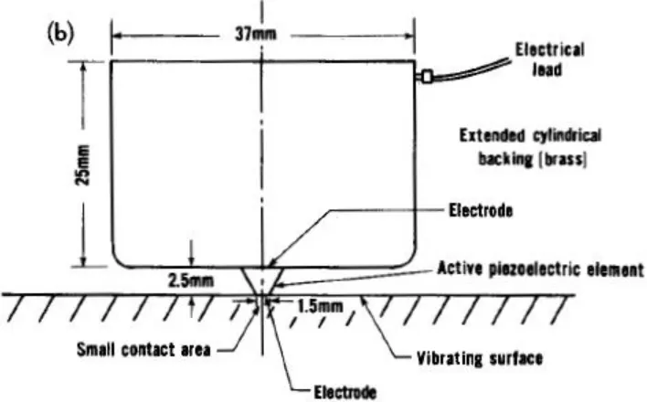
Lamb wave modes interacting with a perfectly bonded PWAS (Giurgiutiu 2014) .. 44 Figure 4.3 Concpetual sketch highlighting components of an ultrasonic transducer

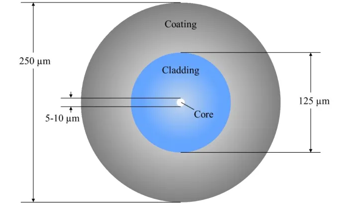
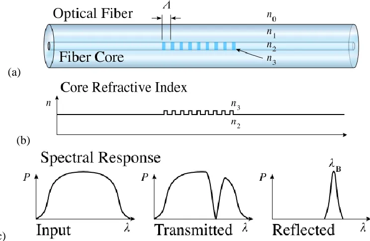
(Nakamura 2012) ... 48 Figure 4.4 NBS conical AE sensor (Proctor 1982) ... 53 Figure 5.1: Dimensions and composition of a single mode optical fiber ... 60 Figure 5.2 (a) Illustration of an FBG within an optical fiber, (b) variation in refractive

index within fiber core, (c) spectral response of an FBG (“Fiber Bragg Grating,” n.d.); used under CC license https://creativecommons.org/licenses/by/3.0/ ... 62 Figure 5.3: Intensity demodulation approach for FBG dynamic strain sensing (Norman

and Davis 2011) ... 64 Figure 5.4: Spectrum of a pi-phase shifted FBG (Rosenthal, Razansky, and Ntziachristos

2011) ... 66 Figure 5.5: Fabry-Pérot interferometer (a) optical resonance cavity formed between two

partially reflective surfaces (“Pérot Interferometer,” n.d.), (b) external Fabry-Pérot interferometer; used under CC license

Figure 7.2: Instrumentation schematic for the FBG optical interrogation system and data acquisition equipment ... 92 Figure 7.3: Cantilever beam specimen for static strain testing (Frankforter, Lin, and

Giurgiutiu 2014) ... 95 Figure 7.4: Relationship between laser output power and RMS noise ... 99 Figure 7.5: (a) FBG response via Luna Phoenix 1400 laser with 10 mW output power,

and (b,c) FBG response via Keysight N7714A laser with 10 mW and 4 mW output power, respectively ... 100 Figure 7.6: 100 kHz ring sensor outfitted with PWAS on top and bottom and a

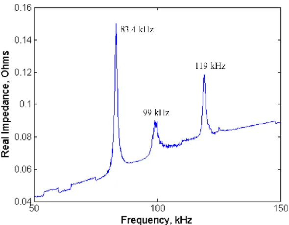
side-bonded FBG ... 102 Figure 7.7: (a) EMIS response of PWAS #1 showing dominant resonances about 100

kHz, and (b) EMIS response of PWAS #2 showing a clearer signal with similar peaks compared to PWAS #1 ... 103 Figure 7.8: Chirp response of the ring sensor in (a) time domain and (b) frequency

domain ... 105 Figure 7.9: (a, c) Time and frequency domain for a three count tone burst, and (b, d) time and frequency domain for a 64-count tone burst ... 107 Figure 7.10: Effect of number of tone burst counts on sensor response amplitude ... 107 Figure 7.11: Experimental setup for plate-bonded ring sensor testing with longitudinal

and transverse PWAS 150 mm away, and a cluster of sensors for testing ... 110 Figure 7.12: EMIS of the stainless steel 100 kHz ring sensor bonded to a 1.2 mm

aluminum plate ... 111 Figure 7.13: Chirp response in (a) time domain, and (b) frequency domain for the

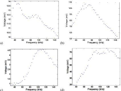
plate-bonded stainless steel ring sensor FBG, excited by the ring sensor PWAS ... 111 Figure 7.14: A0 Lamb wave mode tuning curve for (a) bonded PWAS, (b)

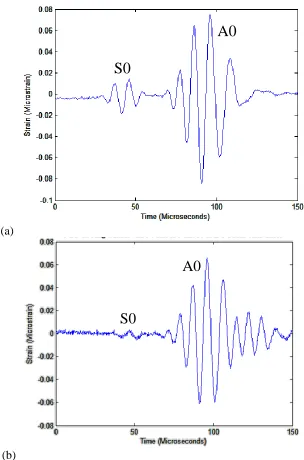
plate-bonded FBG, (c) ring sensor PWAS, and (d) ring sensor FBG ... 113 Figure 7.15: (a) Plate-bonded FBG sensing both S0 and A0 Lamb wave modes, and (b)

ring sensor FBG sensing predominantly the A0 Lamb wave mode ... 115 Figure 7.16: Ratios between in-plane (u_x) and out-of-plane motion (u_y) for S0 and A0

Figure 7.17: Longitudinal and transverse PWAS Hanning window tone burst 99 kHz excitations, sensed by (a,b) plate-bonded FBG, and (c,d) ring sensor FBG ... 117 Figure 7.18: 100 mm longitudinal PLB sensed detected by (a,b) PWAS in the time and

frequency domain, and (c,d) ring sensor PWAS in the time and

frequency domain ... 119 Figure 8.1: (a) 100 kHz ring sensor, (b) fundamental breathing-type resonance nominally at 100 kHz modeled at 107 kHz, and (c) second breathing-type harmonic modeled at 268 kHz ... 131 Figure 8.2: Additional (a) shear-like and (b) torsional-like ring sensor modes near 100

kHz ... 132 Figure 8.3: Harmonic response of the ring sensor to antisymmetric line force excitations

via (a) nominal FBG strain calculated via differential displacement of the two ring sensor FBG holes, and (b) Von Mises strain at the top of the ring sensor ... 133 Figure 8.4: (a) Aluminum and (b) stainless steel broadband frequency response of the 100

kHz aluminum and stainless steel ring sensors ... 135 Figure 8.5: Mode selectivity feature of the ring sensor in capturing transient Lamb waves via (a) response to an incident S0 Lamb wave mode, and (b) response to an incident A0 Lamb wave mode ... 138 Figure 8.6: (a) Strain of a centrally-bonded FBG on a ring sensor shows a theoretical

amplification over (b) longitudinal surface strain detectable by FBG at the same sensing location in a separate plate model ... 139 Figure 8.7: Ring sensor directional dependence. The ring sensor shows a

cosinusoidal-like directional dependence, shifted upwards by a constant ... 140 Figure 8.8: Wavelength of S0 and A0 Lamb wave modes for a 1 mm thick Aluminum

2024-T3 Plate ... 142 Figure 8.9: FEM simulation of ring sensor frequency response with (a) PWAS flush with

the top surface, and (b) PWAS overhanging by 1 mm ... 144 Figure 8.10 (a) Previous ring sensor configuration with a wrap-around electrode and a

Figure 8.12 Chirp excitation of the 100 kHz aluminum ring sensor across a 0-1000 kHz frequency range, (a) time-domain response, and (b) frequency domain response . 147 Figure 8.13: Plate used in ring sensor Lamb wave experiments showing (a) testing area

surrounded by wave absorbing clay, and (b) close-up of aluminum (front) a stainless steel (back) ring sensors ... 149 Figure 8.14: A0 mode tuning curves for (a, b) longitudinal and transverse propagation to

plate-bonded PWAS, (c, d) longitudinal and transverse propagation to aluminum ring sensor PWAS, and (e, f) Longitudinal and transverse propagation to the

aluminum ring sensor FBG ... 150 Figure 8.15: Longitudinal Pitch-catch results for FBG on (a) an aluminum and (b) a

stainless steel ring sensor ... 152 Figure 8.16: Tone burst count sweep experiment to assess the potential for resonance

amplification via the fundamental resonance mode ... 153 Figure 8.17: Response to 100 mm PLB-AE via (a, b) plate-bonded FBG longitudinal time

and frequency response, (c, d) aluminum ring sensor FBG longitudinal time and frequency response, and (e, f) aluminum ring sensor FBG transverse time and frequency response ... 155 Figure 8.18: 100 mm longitudinal steel ball impact detected via (a, b) plate-bonded

PWAS time and frequency response, (c, d) stainless steel ring sensor PWAS time and frequency response, (e, f) aluminum ring sensor PWAS time and frequency response, and (g, h) aluminum ring sensor FBG time and frequency response ... 157 Figure 9.1: (a) 1 N distributed harmonic out-of-plane load applied at the base of the ring

sensor, and (b) example mesh from sensitivity analysis and goal driven

optimization ... 162 Figure 9.2: Effect of (a) ellipse major diameter, (b) ellipse minor diameter, (c) ring depth, and (d) flat height on 1st resonance frequency ... 164 Figure 9.3: Effect of (a) ellipse major diameter, (b) ellipse minor diameter, (c) ring depth, and (d) flat height on 1st resonance amplitude ... 165 Figure 9.4: Sketch of ring sensor geometric parameters ... 167 Figure 9.5: Spearmen correlation coefficients (sensitivities) between ring sensor

geometric features and 1st _{resonance frequency and amplitude ... 167}

Figure 9.7: Geometry of a miniature 100 kHz ring sensor ... 171 Figure 9.8: Harmonic response to out-of-plane motion at 100 kHz for a 3.2 mm outer

diameter ring sensor design ... 172 Figure 9.9: (a) Thicker stainless steel tubing for prototype practice and aluminum tubing

for prototyping, (b) aluminum tubing with flat faces milled and FBG holes drilled, and (c) final ring sensor prototypes... 173 Figure 9.10: Miniature 100 kHz microscopic geometry measurements for (a) inner and

outer diameter, (b) angle between the two flat faces, (c) ring depth, hole size, and hole placement, and (d, e) top and bottom flat surfaces ... 174 Figure 9.11 FEM modal and harmonic analyses of ring sensor with dimensions

back-substituted from microscopic measurements ... 176 Figure 9.12: Effect of material properties and scaling factor on first ring sensor resonance frequency ... 177 Figure 9.13: Miniature ring sensor and original 100 kHz ring sensor comparison and

instrumentation ... 178 Figure 9.14 Electromechanical admittance of the (a) 8.0 and (b) 3.2 mm ring sensors,

chirp response of the (c) 8.0 and (d) 3.2 mm ring sensors, and pitch-catch response of the (e) 8.0 and (f) 3.2 mm ring sensors, respectively ... 179 Figure 9.15: Sensor cluster for sensor evaluation via Lamb wave testing ... 180 Figure 9.16 Longitudinal tuning curves of (a) the original ring sensor and (b) the

miniature mm ring sensor, and transverse tuning curves of the (c) original ring sensor and (d) the miniature ring sensor ... 181 Figure 9.17: A high SNR is observed for sensors responding to a 150 mm PWAS

excitation for (a) the miniature mm ring sensor FBG, as compared to (b) the plate-bonded FBG and (c) the plate-plate-bonded PWAS response ... 184 Figure 9.18: No difference in miniature ring sensor FBG tension/compression behavior

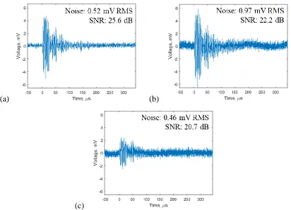
was observed when comparing two Hanning windowed tone burst excitations, one the negative of the other ... 185 Figure 9.19: longitudinal PLB-AE waveforms sensed by (a, b) PWAS on the plate, (c, d)

Figure 9.21: (a,b) Time and frequency optical system noise, and (c) effect of sensing bandwidth on optical system noise ... 192 Figure 9.22: Effect of filtering on the miniature ring sensor FBG pitch-catch response, (a) raw signal and (b) filtered signal ... 193 Figure 9.23: Filtered PLB-AE responses for (a) PWAS on the plate, (b) FBG on the plate, (c) FBG on the 8 mm ring, and (d) FBG on the 3.2 mm ring. ... 194 Figure 9.24: Aluminum test specimen in MTS grips for fatigue test ... 197 Figure 9.25: Data acquisition system setup for fiber-optic static strain and AE tests .... 197 Figure 9.26: Microscopic measurements indicated the fatigue crack length was 17.6

mm. ... 198 Figure 9.27: (a) Aluminum specimen outfitted with sensors in tensile loading frame, and

(b) FBG and PWAS bonded symmetrically about a fatigue crack ... 199 Figure 9.28: Static FEM of the aluminum plate fatigue-AE specimen ... 200 Figure 9.29: FEM calculations of transverse strain variation explain the deviations in the

FBG spectrum observed at high loads ... 201 Figure 9.30: PLB waveforms to establish functionality of the FBG equipment for (a) FBG

5 mm away from the crack, and (b) PWAS 5 mm away from the crack ... 202 Figure 9.31: Tunable laser fixed wavelength set slightly off maximum load for maximum FBG sensing coverage during fatigue loading ... 203 Figure 9.32: (a) Front side of specimen with ring sensor and PWAS, and (b) back side of

specimen with R15α sensor ... 204 Figure 9.33: 0.070 nm wavelength shift observed from miniature ring sensor FBG (a)

under 0 kN load, and (b) under 16.0 kN load ... 204 Figure 9.34: An additional ring sensor and PWAS bonded within 1 mm of the crack tip

and further fatigue experiments were performed ... 206 Figure 9.35: Chart of AE hits, with waveform amplitude (dBmV) on the vertical scale and

time (seconds) on the horizontal scale ... 207 Figure 10.1: The ABH geometry with its thickness following a power law profile

Figure 10.2: (a) ABH height, (b) wavenumber, (c) wave speed, and (d) wavelength calculations for a 50 kHz flexural wave propagating in a 304 stainless steel quadratic ABH ... 221 Figure 10.3: (a) Reflection coefficient as a function of frequency for a 5 mm length and 5

mm height ABH, and (b) reflection coefficient as a function of ABH length for a 5 mm height ABH and an excitation frequency of 100 kHz ... 222 Figure 10.4: 1st resonance frequency of a parabolic tapered sensor ... 227 Figure 10.5: (a) High displacement observed in harmonic analysis without optical fiber

and (b) diminished displacement observed in harmonic analysis with optical

fiber ... 228 Figure 10.6: Load application for dynamic stiffness exploratory FEM models as (a)

distributed harmonic load per unit area applied along the circular cross sections of the optical fiber, and (b) distributed harmonic load per unit length applied along an inner line across the ABH sensor depth ... 229 Figure 10.7: Dynamic stiffness exploratory FEM models where (a) a half-ring sensor had a higher dynamic stiffness than optical fiber, (b) a half-ring had a dynamic stiffness matched with the optical fiber, and (c) a half-ring with dynamic stiffness lower than the optical fiber ... 231 Figure 10.8: Harmonic response of the half-ring geometry with tip thickness tuned for

matched dynamic stiffness, (a) without the optical fiber, and (b) with optical

fiber ... 231 Figure 10.9: (a,b) Sample mesh for a circular ABH sensor variable meshing scheme, (c) 1

N distributed out-of-plane harmonic load along the sensor base, and (d) geometric parameters for a circular ABH sensor optimization... 232 Figure 10.10: Pearson correlation coefficients (sensitivities) for a sensitivity analysis with bounds ±10% of an initial design with 10.0 mm width, 5.0 mm depth, 2.0 mm base height, and 100 µm tip thickness ... 233 Figure 10.11 Local sensitivity plots for ABH sensors with (a) 12 mm width and (b) 6 mm width ... 234 Figure 10.12: Effect of width and base height on (a) 1st resonance frequency and (b) 1st

resonance amplitude ... 235 Figure 10.13: Analysis history of (a) Amplitude output, (b) frequency output, (c) width

Figure 10.14: Final ABH sensor design shown via (a) CAD drawing of 100 kHz ABH sensor, and (b) harmonic analysis frequency sweep of directional deformation of the ABH tip ... 237 Figure 10.15: Conceptual sketch of (a,b) noncontact FPI ABH sensor configurations and

(c) point-contact FBG configuration ... 238 Figure 10.16: 138 kHz mode of in-plane sensitive mode with ABH tips vibrating in

phase ... 240 Figure 10.17: (a) CAD drawing of a 10 kHz ABH resonator, and (b,c) ABH resonator

prototyped in USC machine shop ... 241 Figure 10.18: (a) Sensing performed by an LDV mounted to a 2D translational stage, and

(b) a shaker table mounted on a rotatable fixture to obtain velocity data from

different directions ... 242 Figure 10.19: (a,c) Direction of bolt excitation and sensing, and (b,d) frequency sweep of measured bolt velocity ... 243 Figure 10.20: (a) Direction of excitation and LDV sensing, (b) calibrated response from

100 Hz – 11 kHz, and (c) calibrated response from 14.5 kHz – 20 kHz ... 244 Figure 10.21: (a) Scanning direction of LDV sensing, and (b) four mode shapes across

the span of the ABH tip ... 245 Figure 10.22: (a) An area scan was used for experimentally evaluating mode shape

comparison, and (b) FFT amplitude at its maximum point for each frequency... 246 Figure 10.23 (a, b) “Axial” mode predicted at 10.0 kHz and measured at 6.2 kHz, (c, d)

“axial” mode predicted at 19.1 kHz and measured at 15.8 kHz, (e, f) “flexural” mode predicted at 17.1 kHz and measured at 15.8 kHz, and (g, h) “flexural” mode

predicted at 22.9 kHz and measured at 24.1 kHz... 247 Figure 10.24: (a) Sensor prototype with bonded PWAS and point-contact bonded FBG,

and (b) microscopic sensor geometry measurements ... 249 Figure 10.25: Circular ABH sensor (a,b) chirp response time and frequency domain, (c)

PWAS EMIS response, and (d) FBG response to 150 kHz excitation via PWAS on the sensor base ... 250 Figure 10.26: (a) LDV measurement at the tip of the ABH sensor, and (b) ABH sensor

attached to screw-adjusted mechanical stage ... 251 Figure 10.27: ABH tip velocity in response to 0-1000 kHz chirp excitation (a) with no

Figure 10.28: (a,c) Circular ABH senor mesh and (b,d) quadratic ABH sensor mesh ... 253 Figure 10.29: (a) 1st resonance of circular ABH sensor, and (b) 1st resonance of quadratic ABH sensor ... 253 Figure 10.30: 1st resonance mode of (a) the circular ABH sensor and (b) the quadratic

ABH sensor ... 254 Figure 10.31: Correlation between average displacement and maximum displacement

objective functions ... 256 Figure 10.32: Change in local sensitivity curves at different points in the design space

indicate that some of the parameter effects are non-monotonic ... 257 Figure 10.33: No significant effect of power law exponent on ABH sensor amplitude . 258 Figure 10.34: Quadratic ABH sensor design ... 258 Figure 10.35: (a) ABH power law cut using 3-axis CNC mill, and (b) final ABH sensor

prototype ... 259 Figure 10.36: 1 mm plate for Lamb wave directional experiments ... 260 Figure 10.37: ABH sensor response to 300 kHz tone burst ... 261 Figure 10.38: Angular response of ABH sensor to (a) S0 wave mode, and (b) A0 wave

mode ... 262 Figure 11.1: Steel rail calibration (a) Conceptual sketch of excitation and sensors, and (b) photograph of steel rail during experimental setup ... 271 Figure 11.2: Group velocity calculations via time of flight measurements indicating

Rayleigh wave propagation in the steel rail ... 272 Figure 11.3 (a) Side-by-side comparison of 0.5 mm pencil lead and 0.5 mm OD glass

capillary rod, and (b) pencil lead break fixture recommended in ASTM E976 to improve reproducibility of pencil-lead-break excitations ... 273 Figure 11.4: Capillary rod excitation detected by a PWAS 20 mm away (a) time-domain

response, and (b) frequency-domain response ... 273 Figure 11.5: PLB excitation, detected by a PWAS 20 mm away (a) time-domain

Figure 11.6: (a, b) PWAS 500 ns pulse excitation smoothed due to data acquisition equipment, and (c, d) pitch-catch response detected by a PWAS 394.5 mm away from the transmitter PWAS ... 276 Figure 11.7: Verification of calibration method by comparing experimentally-derived

calibration curve with manufacturer-provided calibration curve for two R15α

sensors ... 278 Figure 11.8: PWAS pulse response, received by (a,b) R15α sensor and (c,d) miniature

ring sensor FBG ... 279 Figure 11.9: (a) Photo of surface-bonded FBG, and (b) Surface-bonded FBG calibration

curve expressed in FBG strain per unit input velocity ... 282 Figure 11.10: (a,c,e) Original 100 kHz ring sensor bonded to steel rail, its calibration

curve, and its strain amplification curve, and (b,d,f) Miniature ring sensor bonded to steel rail, its calibration curve, and its strain amplification curve ... 284 Figure 11.11: Comparison between single-point bonded and two-point bonded

configurations on miniature ring sensor... 286 Figure 11.12: Comparison between miniature ring sensor FBG calibration curves

generated by tone bursts and pulse excitation ... 287 Figure 11.13: (a, c) Surface bonded PWAS and its calibration curve, and (b, d) miniature

ring sensor PWAS and its calibration curve ... 288 Figure 11.14: (a) Optical fiber bonded at one point on ABH face close to the very tip of

the sensor, (b) Optical fiber bonded at one point on the ABH tip, and (c) Optical fiber bonded to both ABH tips in a buckled configuration ... 289 Figure 11.15: Increase in sensor sensitivity by bonding the FBG to the ABH sensor

tip ... 290 Figure 11.16: Strain amplification ratio of a single-point bonded ABH sensor FBG .... 291 Figure 11.17: (a) Calibration curve of the two-point bonded ABH sensor is wideband and relatively flat, and (b) strain amplification ratio of the two-point bonded ABH sensor is higher than any of the other sensor configurations investigated ... 291 Figure 11.18: Calibration curve comparison between most sensitive ring sensor and most

CHAPTER

1

I

1.1MOTIVATION

Risks and costs have been mounting with the prolonged use of aging infrastructure, presenting a clear need for innovative damage monitoring technologies. These same technologies present opportunities within the aerospace industry to monitor aging fleets and to support the usage of composite materials in the next generation of aircraft. To name a few prominent cases:

• Almost one quarter of US bridges are classified as structurally deficient or functionally obsolete, with an estimated $31.6 trillion needed for remediation (U.S. Federal Highway Administration, 2014). Technology which ensures structural reliability with prolonged use can increase safety and reduce remediation costs

• Postponement of the United States national nuclear waste repository has necessitated extensions of on-site nuclear storage. Monitoring of nuclear dry cask storage canisters will be necessary to mitigate failure risk since their use has been extended past their intended design lifespans (Hamilton et al. 2012; Sun 2015)

composites by weight. However, inspection costs of aerospace composites are very high, representing approximately a full third of their lifecycle costs (Diamanti and Soutis 2010).

The emerging field of structural health monitoring (SHM) seeks to address such concerns by supplementing manual scheduled inspection with continuous in situ

monitoring (Giurgiutiu 2014). Many technologies have the potential for use in SHM applications, many of them transitioned from the well-established field of nondestructive evaluation (NDE). The distinction between the two fields relates to the development and use of damage detection technology for continuous monitoring in SHM, or for periodic inspection in NDE.

SHM is incredibly demanding in its scientific and technological challenges. However, there is a strong case for its development and application. In some cases, conventional inspection approaches are difficult or impossible (e.g. in extreme temperatures, explosive environments, and space applications). Continuous monitoring presents the potential to increase assurances of reliability, reducing structural downtime and high costs by decreasing the requisite number of manual inspections. SHM also has the potential to catch unexpected damage in-service with potential savings in money, structures, and lives. From a long-term outlook, SHM can enable advanced design paradigms such as the digital twin, where damage information is used to update a high-fidelity model of an aerospace vehicle. This would allow digital testing of operations and maneuvers prior to execution during flight (Glaessgen and Stargel 2012).

material interfaces, traveling long distances to interact with damage and carry damage-related information. In some cases, guided waves can be initiated by damage events itself such as impacts and acoustic emissions from crack growth. These waveforms are detected by an ultrasonic sensor and can be subsequently interpreted to obtain information about the damage state.

Over the past several decades, there has been a great deal of interest in advancing fiber-optic sensors for ultrasonic sensing as an alternative to conventional piezoelectric sensors. This is because fiber-optic sensors possess many inherent advantages that piezoelectric sensors do not. Fiber-optic sensors are immune to electromagnetic interference and ideal for monitoring in explosive environments. They are corrosion resistant, lightweight, and possess an exceptional form factor. They also possess the advantages inherent in fiber-optic telecommunication technologies such as multiplexing and remote interrogation.

Despite their advantages, fiber-optic technology is not yet mature enough to be in widespread use for ultrasonic guided wave applications. Currently, there are several technical limitations associated with fiber-optic sensors. Some of the most pressing limitations are:

1. Ultrasonic fiber-optic sensors have lower sensitivity and higher noise than their piezoelectric counterparts. This inhibits their ability to detect waveforms associated with small flaws before they begin to cause problems with structural reliability 2. For ultrasonic strain or displacement sensing, fiber-optic sensors tend to only detect

in guided wave applications where waveforms can arrive from any number of incident angles

3. Some of the most promising fiber-optic sensing configurations cease to operate in the presence of static strain. For common implementations such as surface-bonded fiber-optic sensor, this precludes their use for monitoring a structure in-service. Developments in fiber-optic sensing technology which mitigate these limitations help shift the cost-benefit analysis towards feasibility in SHM applications.

1.2RESEARCH SCOPE AND OBJECTIVES

1.2.1 Research Scope

The scope of the research presented in this dissertation is to address fundamental limitations of ultrasonic fiber-optic sensors through a mechanical design approach, where a fiber-optic sensing element is combined with a mechanical resonator. This includes the steps necessary to design, model, verify, characterize, and optimize these mechanically amplified fiber-optic sensors. The emphasis is on guided wave sensing due to its potential for SHM applications.

1.2.2 Research Objectives

• Mechanical resonance amplification to increase sensitivity as compared to a surface-bonded fiber-optic sensor

• Omnidirectional sensing, i.e. ability to sense waves from any incident angle

• Insensitivity to quasi-static strain

• Sensitivity to in-plane motion, out-plane motion, or both by design

• Small sensor size

Since this dissertation started with a sensor candidate in-hand, the first goal was to develop a proof of concept for a resonant mechanical fiber-optic sensor. This involved calibration of a fiber-optic sensing system as well as experiments on both the free sensor and Lamb wave sensor response experiments. The next objective was to characterize the sensor experimentally, guided by theories of guided wave propagation.

A finite element modeling (FEM) framework was a key feature of this project, both for understanding a sensor’s mechanism of action and improving the sensor performance. A FEM-based design exploration and optimization framework was performed for each sensor developed, with the goal of maximizing sensitivity through mechanical amplification.

Finally, one of the biggest gaps identified in a review of fiber-optic mechanical sensors (Chapter 6) was the lack of measured or transferrable performance standards with respect to sensitivity. To this end, one objective of this work was to calibrate the sensors in this work, developing quantitate metrics of sensor performance that both allow for internal comparisons and refer sensor motion back to surface motion of its host structure.

It should be noted that intent of the work presented in this dissertation is to develop mechanical fiber-optic sensors which are generally suited for the detection of ultrasonic guided waves. Some of the research framework presented herein may be skewed more towards AE applications. However, that is because its long history and development provide powerful tools for sensor characterization which are broadly applicable to ultrasonic guided wave sensing.

1.3ORGANIZATION OF THIS DISSERTATION

Chapter 2 of this dissertation presents a review on structural health monitoring and ultrasonic guided waves. Chapter 3 provides a review of acoustic emissions.

Chapter 4 presents a review of ultrasonic NDE and SHM sensors, with an emphasis on piezoelectric wafer active sensors (PWAS), conventional ultrasonic transducers, and acoustic emission sensors.

Chapters 5 and 6 present information in fiber-optic sensors. Chapter 5 presents general principles of fiber optics and fiber-optic sensors to help provide a reader with a background on the topic as applied to ultrasonic sensing. Chapter 6 presents a survey on fiber-optic guided wave sensing with an emphasis on mechanical fiber-optic attachment.

combined with a fiber Bragg grating (FBG) sensor and PWAS. Chapter 7 also includes optical system characterization and calibration.

Chapter 8 presents the use of FEM simulations for free sensors and Lamb wave to investigate the ring sensor mechanisms of action. FBG placement, and PWAS placement and type were studied.

In Chapter 9, a design optimization was performed for both miniaturization and sensitivity enhancement of the ring sensor. The miniature ring sensor prototype is verified experimentally.

In Chapter 10, a wave trapping acoustic black hole (ABH) concept is adapted for sensing applications. A concept of a point-contact bonded optical fiber waveguide is combined with the ABH local vibration. Preliminary experimental investigations were performed.

In Chapter 11, a review on AE sensor calibration methodology is performed, followed by calibration experiments for the sensors developed in this dissertation to put the work performed herein on a better absolute quantitative and transferrable footing.

CHAPTER

2

S

H

M

G

W

R

2.1ULTRASONIC STRUCTURAL HEALTH MONITORING

The developments of this dissertation fall within the scope of ultrasonic SHM, one of the most prominent and promising approaches for damage monitoring. In ultrasonic SHM, permanent structurally embedded transducers transmit and receive ultrasonic guided waves. These waves have the potential to propagate over large areas to interact with damage. Waves that have interacted with damage propagate to a sensor; the detected waveform can be analyzed to determine damage location, type, severity, and even geometry. In some cases, the energy that constitutes the waves can originate from the damage itself, such as from impact and acoustic emission (AE) events.

Interpreting waveforms to characterize damage is fundamentally an inverse problem. This has motivated a growing body of research to develop high fidelity models which represent the forward problem of wave propagation and wave-damage interaction (Poddar and Giurgiutiu 2016). This is further supplemented by data-driven waveform analysis approaches trying to bypass the physics of the problem by using machine learning, parametric correlation, and baseline signal comparison.

damage. Analogously for the SHM system, elastic waves are detected by a structurally embedded sensor, and optical or electrical connectors transmit the information to a computer which interprets the signals as damage-related through data processing algorithms. For the SHM system to be successfully, the embedded sensor must be sufficiently sensitive to damage-induced waves, and the algorithms must be able to judiciously segregate damage-related from non-damage-related events.

2.1.1 Active and Passive SHM Approaches

SHM methods can be divided into two broad categories: passive SHM and active SHM. In passive SHM, no energy from a transducer is input into the structure; rather sensors just “listen” to the structure and are used to infer structural health. In active SHM, an embedded transducer inputs energy into the structure. This excites a wave which interacts with damage, and is subsequently detected by the same or another transducer. A conceptual sketch of several common active and passive ultrasonic guided wave SHM methods is shown in Figure 2.1 (Giurgiutiu 2016). In this figure, the emphasis is on a prominent SHM sensor called a piezoelectric wafer active sensor (PWAS) which is described in more detail in Chapter 4.

2.1.2 Active SHM – Pitch-Catch, Pulse-Echo, and Phased Array

scattered portion of the wave is sensed by the same transducer. In a phased array setup, a group of transducers are placed in distinct spatial locations, and multiple transducers are excited to act as spatial filters using beamforming algorithms. This allows for the scanning of regions across space.

Figure 2.1: Methods of PWAS damage monitoring (Giurgiutiu 2010) 2.1.3 Passive SHM – Impact and Acoustic Emission Methods

wave speeds. In composites, the frequency components can correlate to characteristic types of damage. Although this could be considered impact detection (detecting damage associated with impact), it can also be considered a form of AE sensing as the damage-induced waveform itself is an AE.

AEs are elastic waves generated when a material incurs changes in its internal structure, often associated with damage. They can be associated with cracks, plastic deformation, delamination, fretting, etc. AE is considered a field in its own right, with its own equipment, terminology, analysis methods, and commercial applications. AE sensing is challenging in understanding and interpretation. Application of AE techniques often has components of statistical parametric analysis, clustering algorithms, and damage localization; the question of the exact dynamics of wave propagation is often not assessed. Although recently, there have been trends to characterize source mechanics and wave dynamics in AE for better understanding and predictive power. Improving the forward modeling process is a critical step in advancing the use of AE for SHM sensing, as it allows for a quantitative assessment of the AE-damage relationship, particularly for use in advanced materials such as composites. The theory and application of AE is central to this work and is presented in detail in Chapter 3.

2.2REVIEW OF ELASTIC WAVE PROPAGATION

2.2.1 Axial and Flexural Waves in Bars and Beams

discussion of dispersion phenomenon. An important note is that axial and flexural wave formulations are approximations to the more accurate elastic wave formulations.

Axial waves: For an axial wave in a bar, assume a uniform, elastic, isotropic bar undergoes motion ( , )u x t along the bar’s axial direction. The motion in the bar is prescribed

by the wave equation

2

c u u (2.1)

where the wave speed in the bar

c

 or 2 E

c



 for a uniform bar, E

being the elastic modulus,

m

A method of solving (2.1) is given by the d’Alembert solution where the displacement is equal to the superposition of a forward and backward propagating wave, i.e.

( , ) ( ) ( )

u x t g x ct  f x ct (2.2)

The initial value problem consists of finding the solution to (2.1) subject to initial conditions

0

0

( , 0) ( ) ( , 0) ( )

u x u x

u x v x



 (2.3)

where applying the d’Alembert solution results in





1 1

( , ) ( ) ( ) ( )

2 2

x ct

x ct

u x t u x ct u x ct v z dz

c

 _{ } 

    



4

''''( , ) 0

a w x t  w (2.5)

where the constant

a

 , E being the elastic modulus, I being the area

moment of inertia, and

m

Assuming harmonic motion w x t( , )w x eˆ( ) i t , a separation of variables solution yields the general solution

( ) ( )

( , ) i x t i x t x i t x i t

w x t Ae   Be   Ce e  De e (2.6)

where the wavenumber  is given by

2 4

4

a



  . Following the relation between wave speed

and wavenumber

c



  (2.7)

the flexural wave speed c_Fis given be

(

F

c   a 



   (2.8)

2.2.2 Dispersion Phenomenon and Group Velocity

In practice, waves have the tendency to travel in discrete “packets” of localized waves traveling as a unit. If the wave is dispersive, then the wave packets travel at a velocity called the group velocity c_g which is defined by

g d c

d

 

 (2.9)

Note that the group velocity differs from the wave speed c. Solving equation (2.8) for



The concepts of dispersion, wave packets, and group velocity are of particular importance for guided waves, as dispersive guided waves (e.g. Lamb waves) naturally break down into a number of separate packets each with their own distinct characteristics. 2.2.3 Straight-Crested Axial and Flexural Waves in Plates

Axial and flexural waves in plates are approximations to elastic plate waves which are useful for their simplicity. The tradeoff is that the conditions of the assumptions must be valid, so their scope is limited in applicability. Straight-crested axial and flexural waves serve as approximations to straight-crested S0 and A0 Lamb wave modes at low

frequency-thickness products. Their formulations are presented here in further detail as they serve as a foundation for modeling the wave propagation in variable thickness plates presented in Chapter 10.

1 1 2 1 1 , 2 1 1 2

xx xx yy zz xy xy

xy xx yy zz yz yz

zz xx yy zz zx zx

E E E G

E E E G

E E E G

                                      (2.10) where 1 2(1 ) G E    (2.11)

Plate waves are formulated under plane stress assumptions (



3D elasticity equations reduce to

1 1 2 1 1 , 2 1 2

xx xx yy xy xy

xy xx yy yz yz

zz xx yy zx zx

E E G

E E G

E E G

                              (2.12)

Solving equations (2.12) for  _xx, _yy, and _xy we obtain

2 2 ( ) 1 ( ) 1 2

xx xx yy

yy xx yy

xy xy E E G                  (2.13)

Under small strain approximations, the strain-displacement relations relating to equation (2.13) are

1

2

xx yy xy

u v u v

x y y x

      _  _

Taking an infinitesimal element of a plate with force resultants (force per unit width) N_x, N_y, N_xy, the force resultants can be obtained by integrating the stresses across the thickness and using equations (2.13) and (2.14)

2 2 2 2 2 2 2 2 1 1 h

x _h xx

h

y _h yy

h

xy _h xy

Eh u v

N dz

x y

Eh u v

N dz

x y

u v

N dz Gh

y x                _  _  _  _       _  _  _   _      _  _    







And, applying Newton’s second law to the infinitesimal element results in

2 2 2 2 xy x y xy N N u h

x y t

N N _v

h

y x t

    _{ }       _      (2.16)

Under the conditions of a straight-crested wave, the motion is constant across a single wave front (taken here as the ydirection) such that

( , , ) ( , ) ( , , ) 0

u x y t u x t

v x y t



 (2.17)

where

u

x

v

2 2

2 2 2

1 xy

x N

N Eh u u

h

x y  x  t



 _{ }  _ 

     (2.19)

This can be rearranged to obtain the wave equation

2 2 2 2 L u u c x t  _

  (2.20)

where c_L is the longitudinal wave speed in a plate given by

2 2 1 1 L E c     (2.21)

Thus, the analysis of a straight-crested axial wave of a plate follows the analysis of a straight-crested axial wave in a bar, only with a different wave speed c_L.

For flexural waves in a plate, the assumptions of Kirchoff-Love plate theory are followed; the plate thickness does not change; straight lines normal to the mid-plane of the plate remain straight and normal after deformation. Under these kinematic assumptions, displacements at any location z along the plate thickness are given by

w u z x w v z y w w          (2.22)

where

w

Substituting (2.23) into (2.13) yields

2 2

2 2 2

2 2

2 2 2

2 1 1 2 xx yy xy

E w w

z

x y

E w w

z x y w zG x y             _  _  _  _       _  _  _   _      (2.24)

The moment resultants (moment per unit width) can be obtained by through integration across the plate thickness h:

2 2 2 2 2 2 2 2 2 2 2 2 2 2

2 (1 )

h

x _h xx

h

y _h yy

h

xy xy

h

w w

M zdz D

x y

w w

M zdz D

x y

w

M zdz D

x y                _  _            _  _           







where D is the plate flexural stiffness, i.e.

3 2 12(1 Eh D  

  (2.26)

Taking an infinitesimal plate element subject to moments and vertical forces, Newton’s second law can be applied to obtain

2 2 0 0 y x xy x x y xy y Q Q w h

x y t

M M Q x y M M Q y x                        (2.27)

2 2

2 2

2 2 2

xy xy y

x M M M

M w

h

x x y x y y  t

  

 _{   } 

       (2.28)

Substituting (2.25) into (2.28):

2 4 4 2

4 2 2 2 4 2 0

w w w w

D h

x x y y  t

    

   

 _{   }  _

  (2.29)

which can be further simplified using the biharmonic under z-invariant conditions

4 2 4

4

4 2 2 2 4

x x y y

  

   

    (2.30)

resulting in

2 4

2 0

w

D w h

t

 

  

 (2.31)

This is the general equation of motion for a flexural wave propagating in a plate. Note that, although Cartesian coordinates were used in the formulation, in general equation (2.31) is not limited to the use of Cartesian coordinates.

When the conditions of straight crested waves are imposed, i.e.

( , , ) ( , )

w x y t w x t (2.32)

equation (2.31) simplifies to

'''' 0

Dw hw (2.33)

This is analogous to the flexural vibration of a beam, admitting the solution

( ) ( )

( , ) i Fx t i Fx t Fx i t Fx i t

w x t Ae   Be   Ce e  De e (2.34) where the flexural wave speed in a plate is given by

1 4 F D c h      

/

F cF





2.2.4 Bulk waves

In an unbounded medium, waves propagate in all directions. This can be modeled using 3D elasticity theory, where a plane wave propagating along a direction

1 1 2 2 3 3

nn e n e n e can be represented by a displacement

( )

u Af n r ct (2.37)

where the amplitude vector A is given by AA e_{1 1}A e_{2 2} A e_{3 3}. Using the 3D linear elastic equations of motion in an isotropic medium, i.e. the Navier-Lamé equations:

2

(     u)  u u (2.38) Substitution of (2.37) into (2.38) and subsequent manipulation yields an eigenvalue problem









0

c c

    

      

  (2.39)

The solution to which is three eigenvalues, two being identical

1 2 3 2 P S c c

c c c

           (2.40)

2.2.5 Wave Potentials

Using Helmholtz decomposition, or Helmholtz’s theorem, a sufficiently smooth

vector field can be expressed in terms of a scalar potential  and a vector potential H

such that

u

   

H

This is accompanied by the uniqueness condition

0

H

 

Application of Helmholtz decomposition is a useful tool in the derivation of many fundamental wave propagation methods, in particular those for guided waves. For bulk waves, equations (2.41) can be substituted into the Navier-Lamé equations (2.38) to express wave propagation in unbound media in terms of wave potentials, i.e.

2

2

P

S c

c H H

   

  (2.43)

In this sense, it can be considered that both the scalar and vector wave potentials follow the wave equation, propagating at the pressure speed and shear speed of the medium, respectively.

2.2.6 Rayleigh Waves

where c_S is the shear wave speed and k is the ratio of wave speeds in the medium, i.e. 2 2 2 2(1 1 2 P S c k c        (2.45)

A common approximation to the Rayleigh wave speed is given by 0.87 1.12

(

1

R S

c  c 





 

  _{ } _ (2.46)

Modeling Rayleigh waves under z-invariant conditions, the particle motion is given by

( ) ( ) ˆ ( , , ) ( ) ˆ ( , , ) ( )

i x t

x x

i x t

y y

u x y t u y e

u x y t u y e

        (2.47)

where x is the propagation direction, and y is along the thickness of the half space. The component ei( x t) represents the forward propagating component of the wave. The mode shapes are given by

2 2 2 2 ˆ ( ) 2 ˆ ( ) 2 y y x y y y

u y Ai e e

u y A e i e

                   _  _       _  _   (2.48)

with the parameters

2 2 2 2 2 2 2 1 1 P S c c c c        _  _      _  _   (2.49)

and c is the real root of equation (2.44).

products in finite thickness plates. Secondly, the polarization of the particle motion is elliptical in nature; that is, the direction of displacement caused by both u_x and u_yrotates in a retrograde fashion (counterclockwise for a wave traveling to the right). An interesting characteristic of Rayleigh waves is that at the surface, the ratio between in uˆ_x and uˆ_y is

constant for a given material (although below the surface, the ratio is frequency-dependent). This constant ratio between in-plane and out-of-plane displacements becomes important for calibration in Chapter 11.

2.2.7 Shear Horizontal Waves

Shear horizontal waves are the simplest elastic plate waves to model, as they do not couple with the pressure or shear vertical waves. SH waves are modeled with propagation along the x-axis, straight-crested with z-invariance, and the thickness along the y-axis. The plate surfaces are traction free at the plate top and bottom surfacesy d. The particle motion only has the u_zcomponent, and is given by

( )

( , , ) ( ) i x t

z

u x y t h y e   (2.50)

where h y( ) is a standing wave across the plate thickness, and ei( x t) represents the forward propagating component. The characteristic equation for SH waves is

sindcosd0 (2.51)

where

2 2 2

S c



  . Equation (2.51) admits solutions which are both symmetric and

antisymmetric about the plate midline. The solutions are symmetric under the condition

0, , 0,1,... 2

S

d n  n

       (2.53)

Each eigenvalue admits a value of , each representing a separate mode in the general solution, which for symmetric modes becomes

 

2

( , , ) cos i x t

S z

u x y t C y e   (2.54)

The solutions are antisymmetric under the condition

cosd 0 (2.55)

which has eigenvalues

, ,5 ,..., (2 1) , 0,1,...

2 2 2 2

A

d    n  n

     (2.56)

Each eigenvalue admits a value of , each representing a separate individual propagating mode in the general solution, which for antisymmetric modes becomes

 

1

( , , ) sin i x t

A z

u x y t C y e   (2.57)

It should be noted that because     , shear horizontal modes are dispersive (except for the first symmetric shear horizontal S0 mode, which has an eigenvalue of 0). At

high frequency-thickness products, the phase velocity and group velocity of both the symmetric and antisymmetric modes asymptotically approach that of the S0 mode.

Not all shear horizontal modes propagate in a plate at a given frequency-thickness product. For low-frequency-thickness products, some wave modes have wave speeds which become imaginary and indicate non-propagation. The lowest frequency-thickness product at which a mode propagates is called the cut-off frequency, and is given by

 

Imaginary modes do not propagate, but exist in a non-propagating form called evanescent modes. These modes form around local discontinuities and serve to meet local boundary conditions, but do not transmit energy or information. For elastic waves, a complete solution must involve purely real modes which propagate, purely imaginary modes which do not propagate, and complex modes which propagate with decaying amplitude.

2.2.8 Lamb Waves

Lamb waves are elastic waves which propagate in finite thickness plates. Unlike axial and flexural plate waves, Lamb waves do not require a low frequency-thickness approximation; rather, they are a direct result of applying linear elastic theory to an isotropic plate with the top and bottom surfaces traction free at y d. This review of Lamb waves in this section assume straight crested propagation along the x-axis with z-invariance, although solutions are readily available for circular crested waves. Lamb waves are more complex in their formulation than shear horizontal waves, as they are formed by coupled pressure and shear vertical waves. Lamb wave are comprised of symmetric and antisymmetric wave modes, analogous to axial and flexural waves, respectively. Symmetric wave modes are symmetric about the plate midline (u_y is equal and opposite),

and antisymmetric wave modes are antisymmetric about the plate midline (u_x is equal and opposite). For the symmetric modes, the displacements are given by









2 2 2

2 2

2 cos cos cos cos

2 cos sin cos sin

i x t

S S

x S s P S S P S

i x t

S S

y p S s P S P S

u iC d y d y e

u C d y d y e

                            _   _  

2 2 2 2 2 2 2 2 P P S S c c           (2.60)

The wavenumbers  of each symmetric mode are eigenvalues from the symmetric Rayleigh-Lamb equation

2 2 2

2 ( ) tan tan 4 S P

S P S

d d        

  (2.61)

where the phase velocity of each mode is given in general by c 



 . Similarly, the

displacements for the antisymmetric modes are given by









2 2 2

2 2

2 sin sin sin sin

2 sin cos sin cos

i x t

A A

x S s P S P S

i x t

A A

y p S s P S P S

u iC d y d y e

u C d y d y e

                           _   _  

 _   _ (2.62)

The wavenumbers



2

2 2 2

4 tan

tan ( )

P S P S S d d    

     (2.63)

A dispersion curve for a Lamb wave is shown in Figure 2.2. Like shear horizontal waves, Lamb waves have cutoff frequencies, frequency-thickness products below which wave modes become imaginary and do not propagate. All symmetric and antisymmetric Lamb wave modes are dispersive, each approaching the Rayleigh wave speed at high frequency-thickness products. The first symmetric mode (S0) and first antisymmetric mode

(A0) at low frequency-thickness products can be approximated by axial and flexural waves,

involve all complex modes. This involves the superposition of symmetric and antisymmetric real (propagating), imaginary (evanescent), and complex (propagating with decaying amplitude) modes.

Figure 2.2: Lamb wave symmetric and antisymmetric dispersion curves (“Lamb Waves,” n.d.); used under CC license https://creativecommons.org/licenses/by/3.0/ 2.2.9 Longitudinal Elastic Waves in Cylindrical Rods

Contrasting with the approximate axial wave solutions for bars and beams, there is a closed form solution for elastic waves in circular rods (Graff 1975) which are better applicable to some wave propagation cases such as wave propagating along an optical fiber waveguide.

The formulation is via the Navier-Lamé equations in cylindrical coordinate r,z