A Novel Approach for the Direct Simulation of Subgrid-Scale Physics in Fire Simulations

ABSTRACT

BALASUBRAMANIAN, SIVARAMAKRISHNAN. A Novel Approach for the Direct Simulation of Subgrid-scale Physics in Fire Simulations. (Under the direction of Dr. Tarek Echekki).

A Novel Approach for the Direct Simulation of Subgrid-Scale Physics in Fire Simulations

by

Sivaramakrishnan Balasubramanian

A thesis submitted to the Graduate Faculty of North Carolina State University

in partial fulfillment of the requirements for the degree of

Master of Science

Mechanical Engineering

Raleigh, North Carolina 2010

APPROVED BY:

DEDICATION

BIOGRAPHY

ACKNOWLEDGMENTS

I would like to thank so many people for helping me in the construction of my Master’s degree. First and foremost, I would like to thank my advisor Dr. Tarek Echekki, for his guidance and support throughout this research. Whenever I knock on his office door, he would patiently clarify all my doubts, in spite of his busy schedule. This research could not have been completed without his brilliant technical expertise, motivation, and enthusiasm. I would like to sincerely thank Dr. William Roberts and Dr. Tiegang Fang for serving on my advisory committee. I would also like to thank the Fire Dynamic Simulator (FDS) group for providing us the LES code and Dr. Shufen Cao for providing us the ODT code.

I would like to specially thank my roommates Nikhil and Krunal (motu) for their continued support and the delicious food they served me. I would like to extend my thanks to my lab mates: Wei Wang, Kamlesh Gupta, and Ji Park. I would also like to thank Sumit Sedhai for helping me in debugging the code.

I would like to express my gratitude towards my sisters – Shobana Karthik and Lakshmi Sivaramakrishnan. Finally, I would like to thank my parents for their motivation, love, and support. They had strong belief in me and they helped me through my tough times. I could not have completed this thesis without them. I dedicate this thesis to them.

TABLE OF CONTENTS

List of Tables ………. viii

List of Figures ………. ix

Chapter 1 Introduction 1.1 Background ………. 1

1.2 Motivation ………... 2

1.3 Large Eddy Simulations (LES) ………... 3

1.3.1 The Linear-Eddy Model (LEM) …………..……….. 4

1.3.2 The One-Dimensional Turbulence (ODT) Approach ……… 5

1.4 Objectives……… 6

1.5 Outline………. 6

Chapter 2 Introduction to LES-ODT Coupling 2.1 Objectives……… 8

2.2 Eulerian Formulation of LES-ODT………. 8

2.3 Lagrangian Formulation of LES-ODT………. 8

2.4 LES-ODT Model Strategy ……….. 9

2.5 LES variables passed to ODT ………. 14

2.6 ODT variables passed to LES ………..………. 15

2.7 The Flame Displacement Speed……….. 15

Chapter 3 LES Formulation and Numerical Implementation 3.1 Objectives……… 16

3.2 LES Grid Cells ……… 16

3.3 The Mixture Fraction ……….. 17

3.3.1 The Stoichiometric Mixture Fraction ……… 18

3.4 LES Governing Equations ………. 19

3.5 FDS Solution Algorithm ………. 22

3.6 Introduction to the FDS source code ……….. 24

3.7 Combustion Model in FDS ………. 24

3.8 Turbulent Viscosity Computation in LES ………. 28

3.9 The Smokeview ……….. 28

Chapter 4 ODT Formulation and Numerical Implementation

4.1 Objectives ………... 31

4.2 ODT Model Strategy………... 31

4.3 ODT Governing Equations ………. 34

4.4 Scalar Computation in ODT……… 35

4.4.1 Viscosity Computation …...……… 35

4.4.2 Mass Diffusivity and Thermal Conductivity Computation…...…….. 36

4.4.3 Density Computation ……….……… 37

4.5 Stirring Processes in ODT ……….. 38

4.5.1 Triplet Mapping ……… 41

4.5.2 Pressure-Scrambling Model ……….. 42

4.6 Molecular Diffusion-Reaction Processes in ODT……… 43

Chapter 5 LES-ODT Formulation and Numerical Implementation 5.1 Objectives……… 45

5.2 Simulation Conditions ……… 45

5.3 Schematics of ODT domain ………... 47

5.4 Minimum and Maximum Positions of ODT domains………. 48

5.5 The Flame Displacement Speed Derivation……… 48

5.6 Flow Variables Initialization for ODT………..51

5.6.1 Temperature and Mass fractions ……….. 51

5.6.2 Velocity ……… 55

5.7 Interpolation ……….. 56

5.8 Filtering operation………... 59

Chapter 6 Results and Conclusions 6.1 Objectives……… 60

6.2 Outputs of the Simulations in Smokeview ………. 60

6.3 Mixture Fraction during the Simulation……….. 63

6.4 Management of ODT Anchor Points ……….. 64

6.5 Transient Plots ……… 66

6.5.1 Temperature ……….. 66

6.5.2 Fuel Mass Fraction …..………. 68

6.5.3 Oxygen Mass Fraction .………. 70

6.5.4 Reaction Rate ……… 72

References ... 76

Appendices ……….. 79

LIST OF TABLES

Chapter 3

Table 3.1 FDS source files and their respective functions ………. 24 Chapter 4

Table 4.1 Constants used in diffusion collision integral ……… 36 Chapter 5

LIST OF FIGURES

Chapter 2

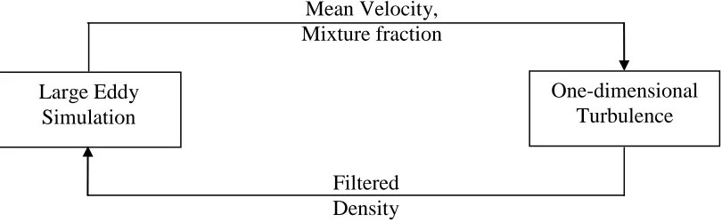
Figure 2.1 Flowchart of flow variables being transferred between LES and ODT …… 10

Figure 2.2 Flowchart of LES and ODT processes implemented together ………. 12

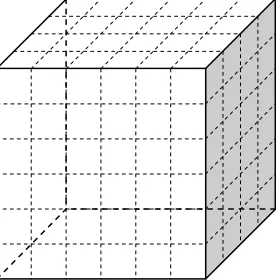
Chapter 3 Figure 3.1 LES domain and grid cell ………. 17

Figure 3.2 Flame extinction criteria used in FDS 5.0 ………. 25

Chapter 4 Figure 4.1 Implementation of ODT process ……….. 33

Figure 4.2 Stirring process in ODT ……… 39

Figure 4.3 Triplet mapping ………. 42

Chapter 5 Figure 5.1 Schematics of ODT domain ………... 47

Figure 5.2 Temperature initialization ………. 54

Figure 5.3 Mass fractions initialization ……….. 55

Figure 5.4 Interpolation of a field variable ………. 58

Chapter 6 Figure 6.1 Snapshots of temporal evolution of jet diffusion flame isosurface on Smokeview ………. 62

Figure 6.4 Management of anchor points in the LES domain………... 65 Figure 6.5 Transient snapshots of temperature at various timesteps

for velocity = 2 m/s and Reynolds number =9300 ……… 67 Figure 6.6 Transient snapshots of fuel mass fraction at various timesteps

for velocity = 2 m/s and Reynolds number = 9300 ……….. 69 Figure 6.7 Transient snapshots of oxygen mass fraction at various timesteps

for velocity = 2 m/s and Reynolds number = 9300 ……….. 71 Figure 6.8 Transient snapshots of reaction rate at various timesteps for

CHAPTER 1 Introduction

1.1Background

Turbulent Combustion is a mixture of two complex phenomena - Combustion and Turbulence. The emergence of Computational Fluid Dynamics (CFD) has really improved our understanding of the complex nature of turbulent combustion. There are three basic approaches to the turbulent combustion. They are Direct Numerical Simulations (DNS), Large-Eddy Simulations (LES), and Reynolds-Averaged Navier-Stokes (RANS) approach (Poinsot and Veynante, 2001).

The DNS is the most accurate representation of turbulent flows. The grids are well refined in a DNS approach and hence, the scalars are directly computed from the refined temporal and spatial grids (Cao and Echekki, 2008). The major disadvantage of DNS is the computational cost, which grows larger, as the problem physical size, extent of chemical complexity, and the size of the chemical mechanism are increased. The grid size is usually in the order of microns in a DNS model for practical hydrocarbon combustion.

widely available in commercial CFD codes, remains the most common solution method for turbulent combustion flows.

The third category is Large Eddy Simulation (LES) approach, which is used in our present study. This method was proposed by Deardorff (1974) for turbulent non-reacting flows. The major concept in LES is that, the large scale turbulent motions are explicitly represented, while the small scale motions are modeled additionally (Pope, 2000). The advantage of LES is that it is more accurate than the RANS approach. The large scale-dynamics are directly modeled; while this method allows the small scale dynamics to be modeled independently (Germano et al., 1991). The computational cost for LES is higher compared to RANS and lower compared to DNS. The accuracy, similarly, for LES modeling is better compared to RANS and not that better compared to DNS. LES has been applied to various scenarios like aircraft engine combustion (Di Mare et al., 2004) and gas turbine combustors (Selle et al., 2004).

1.2Motivation

In combustion, a significant portion of the relevant physics occurs on the subgrid scales and therefore, they constitute an important part of implementing closure in the LES of combustion. Turbulence in turbulent combustion also tends to increase the rate of combustion by increasing the efficiency of mixing. More importantly, to model the processes in the small scales, the resolved scales might not be enough. This leads to the only solution, being direct simulation of these sub-grid scale processes.

The One-Dimensional Turbulence (ODT) model (Kerstein, 1999) offers an important refinement of the LES model. The ODT formulation includes the solution of the reaction-diffusion equations and representations of the stirring events using „triplet maps‟. The ODT model also enables resolution for physics that is not resolved in LES.

The LES-ODT is a modeling framework for the direct simulation of these sub-grid scale physics (Cao and Echekki, 2008). It is a coupling of LES with ODT governing equations at the sub-grid scale level. The coupling involves solving coarse-grained transport equations for LES and subsequently solving, the fine grained ODT transport equations for momentum, species and temperature within the same computational domain. Here, we consider the Lagrangian form of ODT solutions, where we advance the ODT solutions along with the LES.

1.3Large-Eddy Simulations

the reaction in a diffusion flame. We have dealt with jet diffusion flame where the fuel and oxidizer do not meet before the reaction. The configuration is relevant to different fire scenarios. In the sections below, we discuss the recent refinements of the LES combustion in the non-premixed flame model. The recent refinements include one-dimensional methods such as Linear-Eddy Model (LEM) and One-dimensional One-Dimensional Turbulence (ODT) Model.

1.3.1 The Linear-Eddy Model (LEM)

The Linear-Eddy Model (LEM) was originally proposed by Kerstein (1988). This model, unlike the one-dimensional ODT model, is a mixing model. This model was basically a scalar mixing model at first, which, later was used for subgrid mixing (Ochoa and Fueyo, 2009). LEM has the capability of differentiating each physical process such as stirring, advection, and diffusion. LEM was first applied to hydrogen-air combustion (McMurthy et al., 1992) and later for both premixed and non-premixed combustion flows (Menon et al.,

1993).

1.3.2 The One-Dimensional Turbulence (ODT) Approach

The ODT approach was developed by Kerstein (1999). This approach is a refinement of the Linear-Eddy Model. It is a one-dimensional turbulence model, which include turbulent transport stochastically through discrete stirring events and molecular processes in a deterministic way, by solutions of unsteady reaction-diffusion equation along a single-dimensional domain (Kerstein, 1999). This model resolves the computational grid temporally and spatially and solves for the momentum transport, chemistry and advection. The advection is computed using random rearrangement events for scalar fields and momentum using triplet maps, while, the molecular diffusion is computed by solving reaction-diffusion equations along the one-dimensional domain. The stirring event on an eddy is modeled through the triplet maps. Triplet maps are designed to represent the compressive-strain and rotational-folding effects of turbulent eddies in one dimension. The ODT also transports components of the velocity vector, hence, has a mechanism for „driving turbulence‟. The eddy size, location, and distribution are determined by the local field, unlike LEM, and this makes ODT a self-contained turbulence model.

ODT was first implemented in combustion for jet diffusion flames by Echekki et al., (2001). As an Eulerian form, ODT was applied along with LES in autoignition in non homogeneous mixtures (Cao and Echekki, 2008) and the results were validated with DNS simulations. ODT has also been implemented as a standalone model in autoignition of hydrogen in a turbulent jet with preheated co flow air (Echekki and Gupta, 2009).

1.4 Objectives

The main objective of this thesis is to extend the LES-ODT approach to the simulation of fires, develop a code, bridging the LES and ODT and computing the scalars at intermediate LES timesteps. In contrast with the work of Cao and Echekki (2008), the present effort will be based on a Lagrangian formulation for LES-ODT. The LES and ODT solutions are carried out in a three dimensional domain. The ODT domains are attached to the flame brush. The ODT domains are also updated when the LES timestep is being incremented. The reaction mechanism involves a simple and one-step global mechanism for the complete combustion of propane.

1.5 Outline

The remaining part of the thesis is organized as follows.

 Chapter 2 deals with the introduction of LES-ODT coupling.

 Chapter 4 gives a basic concept of the ODT and governing equations of the ODT.

 Chapter 5 deals with the solution implementation of both LES and ODT. Chapter 5 also provides information regarding the way LES and ODT are coupled.

CHAPTER 2

Introduction to LES-ODT Coupling

2.1 Objectives

The main objective of this chapter is to provide a basic insight of the LES-ODT coupling procedure. This chapter also discusses the flow variables that are being passed from LES to ODT and vice versa.

2.2 Eulerian formulation of LES-ODT

The Eulerian formulation of LES-ODT approach was applied in Cao and Echekki (2008). In this approach, ODT solutions were placed in a lattice inside the LES computational domain. As with the definition of Eulerian formulation, the ODT solutions were fixed in space and time. The ODT domains were static and their positions were not updated with the LES timestep. Hence, in Eulerian formulation, the flow properties are a function of fixed position vector and time.

2.3 Lagrangian formulation of LES-ODT

scalar statistics at different timesteps and acts as a closure for the LES formulation. This formulation is related to the Eulerian formulation by the equation (2.1).





D

.

Dt t



  



V V

u V (2.1)

In the equation (2.1), u is the velocity vector and V is any flow vector, D

Dt

V

is called the

Lagrangian derivative or material derivative, t

 

V

is the Eulerian derivative or the partial

derivative.

2.4 LES-ODT Model Strategy

Figure 2.1 – Flowchart of flow variables being transferred between LES and ODT

The whole coupling of LES and ODT is shown in figure 2.2. In figure 2.2, ULES refers to the

velocity in three dimensions in LES, ZLES refers to the mixture fraction in LES, U1D refers to

the velocity in one dimension in ODT, Z1D refers to the mixture fraction in one dimension in

ODT, YF, YO refers to the mass fraction of the fuel and oxygen in ODT, and T refers to the

temperature in ODT.

The process is explained as follows. The LES process is first started. The LES simulations are implemented until the flame gets settled. Then, the ODT process is started once the flame is well established. The time, when the flame gets well established, can be computed by running the model with only LES simulations and a simplified model for combustion. Once the ODT process is started, the code checks for the initialization step. If this is the first time ODT process is started, then the temperature, mass fraction of fuel and oxygen are interpolated from the LES mixture fraction. This ensures initial values for the ODT

Filtered Density Mean Velocity, Mixture fraction Large Eddy

Simulation

Start LES Timestep

ODT Start

Initial ODT

Anchor Points

Compute ODT Grid

Interpolation of U1D from ULES and

Z1D from ZLES

Interpolation of U1Dfrom ULES

No

Yes

Yes

No

Update ODT grid Update anchor

points

YF,YO,T for ODT

from Z1D

Compute ULES and

ZLES

2.5 LES Variables passed to ODT

The LES provides the LES-ODT approach with velocity and mixture fraction solution. The velocities and mixture fraction are computed at each LES timestep after the simulation is started. Initially, the mixture fraction is used to compute the temperature and mass fractions. These flow variables are then interpolated to one-dimension using the interpolation technique discussed in Chapter 5. The ODT solutions are solved, after obtaining values through the interpolation technique.

ODT Solution

End of all LES timestep

Stop No

2.6 ODT Variables passed to LES

The ODT provides scalar statistics for the LES approach. The scalars include the density, which is needed by the LES. The density, that is computed inside the ODT solutions using temperature and mass fractions is then filtered into three dimensions and sent back to the LES. This provides a better approximation to the density compared to the density computation in LES, which follows the ideal gas relations.

2.7 The Flame Displacement Speed

CHAPTER 3

LES Formulation and Numerical Implementation

3.1 Objectives

The objective of this chapter is to describe in detail the LES process. This chapter also discusses the LES governing equations and the combustion model being used in LES. This chapter provides a basic insight of the Fire Dynamic Simulator (FDS), which is used for the LES modeling and the Smokeview, which is used for viewing the outputs of the simulation.

3.2 LES Grid Cells

Figure 3.1 – LES domain and grid cell

3.3 The Mixture Fraction

The mixture fraction is a scalar, defined as the percentage of mass of fuel, in a gaseous mixture (Kuo, 2005). This includes the burned and unburned gaseous mixture. Thus, at a burner surface, the mixture fraction is 1 and in fresh air it is 0. It is denoted by the letter Z. Consider the reaction given below involving combustion of a hydrocarbon,

2 2 2 2 2 2 2 2

x y z a b O CO H O CO S N M

C H O N M  O  CO  H O CO S N  M

Then mixture fraction Z, for the above reaction is given by equation (3.1),





F O O I F O

sY Y Y

Z

sY Y

 

 



 (3.1)

2 2 O O

f f

M s

M

 

 (3.2)

x - direction y - direction

In the equation (3.1) and (3.2), YO is the mass fraction of the Oxygen, YO 

is the ambient mass fraction of the Oxygen (default value = 0.23), I

F

Y is the mass fraction of the fuel at the inlet (default value = 1.0), Y_F is the mass fraction of the fuel, _Fis a constant equal to 1,

2 O

 is the

number of moles of oxygen required for complete combustion of one mole of the fuel, MF is

the molecular weight of the fuel and 2 O

M is the molecular weight of oxygen.

The mixture fraction is a function of space and time. A transport equation is used to resolve the spatial and temporal evolution of the filtered mixture fraction in the FDS code. This scalar can be used to represent all the other species in a chemical reaction. This results in solving one transport equation for the mixture fraction, instead of solving separate transport equations for each species (McGrattan, 2009). This process of computing mass fractions of different species from mixture fraction is called state relations of that species.

3.3.1 The Stoichiometric Mixture Fraction

When the combustion is complete, the stoichiometric mixture fraction indicates the actual flame surface in a diffusion flame, where the fuel and the oxidizer meet.

O st I F O Y Z sY Y     (3.3) 2 2 O O f f M s M    (3.4)

1, 2 O

 is the number of moles of oxygen required for complete combustion of one mole of the

fuel, MF is the molecular weight of the fuel, and MO₂is the molecular weight of oxygen The fuel we have used is propane and calculating the stoichiometric mixture fraction using equation (3.3) and (3.4), we get equation (3.5) and (3.6). The complete combustion reaction of propane is given below.

3 8 5 2 18.8 2 3 2 4 2 18.8 2

C H  O  N  CO  H O N

3.636

s (3.5)

0.0595

st

Z  (3.6)

3.4 LES Governing Equations

The LES Governing Equations that are used in FDS for a Newtonian fluid, taken from the FDS Technical Reference Guide are as given in equations (3.7) – (3.10) (Tannehill, 1997). Equation of Continuity

. m_b t



 _

  

 u (3.7)

Equation of Momentum

 

t    

 _{       }

 u uu g f (3.8)

Equation of Energy

 

t   t 

Ideal Gas Equation RT p W   (3.10)

In the equations (3.7) - (3.10), f_bis the force term representing the external forces on the fluid such as drag forces, qrepresents the conductive and radiative heat fluxes from a chemical reaction, qis the heat release rate per unit volume, q_bis the energy transferred to the evaporating droplets, and  is the dissipation rate. The following quantities are defined as follows:

,

s r

k T h _ D_ Y_ 



   



q q (3.11)

.

ij

  u (3.12)

 

ij ij ij

2 2

3

 _    _

 S u  (3.13)

j i ij j i u u 1

2 x x

    _  _     S (3.14) ij

 is the Kronecker delta, which is defined as: ,

,

ij

1 i j 0 i j

   _ 

  (3.15)

The mass conservation equation is often written in terms of the species conservation equation. This is given in equation (3.16).

 

t         

 _{       }

 u (3.16)

approximation of the equation of state, as shown in equation (3.17), is done by splitting the pressure into background pressure and a perturbation pressure (Rehm and Baum, 1978). This assumption is called as the Low Mach Number assumption.

( , ) _m( , ) ( , )

p x t  p z t p x t (3.17)

In equation (3.17), p_mis the background pressure and pis the perturbation pressure. The divergence in FDS is written as the equations (3.18) – (3.20),

. _{D P} pm

t

   



u (3.18)

m P 1 R P 1 p Wc    _  _   (3.19)





b s b b P b b

P i

Y h

m W W 1 W

D D m Pw g

W W W c T

m R

q q h D Y m Y c T T

Wc p 2

                             _  _ _  _              _           _  









q u u

(3.20)

Applying the above assumptions in the LES governing equations, (3.7) – (3.10), we get equations (3.21) – (3.26),

Equation of Continuity

. .

t

 _{ }



    

 u u (3.21)

Equation of Species

. . .

Y

Y Y D Y m

t                     

Equation of Momentum





. b ij H

t     

 _{ }

     _     _



u

u g f (3.23)

Equation of Pressure

 





F u g f (3.25)

Ideal Gas Equation

 

Y

p z t TR

W 

 







In the equations (3.21) – (3.26), the ω is the vorticity, fb is the body forces, g is the

acceleration due to gravity, ρ is the density, u is the velocity vector, Yβ is the mass fraction of

species β, R is the universal gas constant, H is the total pressure divided by the density, and pm is the background pressure. The source terms of the energy equation are added to the

divergence term, “.u”as shown in equation (3.18).

3.5 FDS Solution Algorithm

(3.27) – (3.29) refers to the predictor step. The thermodynamic quantities such as density, pressure and mass fractions are estimated at the next timestep using explicit Euler method as shown in equation (3.27).

 





. .

P

t t t t t t t

t

    

   u   u (3.27)

These thermodynamic quantities lead to the formation of the divergence at the next timestep. The pressure is then solved directly using the Poisson solver as shown in equation (3.28).

 

 

 

.

P P

t t t

t t 2 t H t                  u u F (3.28)

The velocity is then estimated using equation (3.29)

t t_P t t t t_P

t H

 _{     }  _

 

u u F (3.29)

The timestep is checked after the predictor stage to satisfy the stability criterion. The above flow properties are corrected in the corrector steps as shown in equations (3.30) – (3.32). The same set of steps is followed in the corrector stage to correct the flow properties.

   





. .

P P P P P

t t t t t t t t t t t t 1 t

t 2

  _  _  _{ }  _  _  _  

 u u  (3.30)

 

 

 

 

.

P

P

t t t t t

t t t t 2 2 H t                     

u u u

F (3.31)

t t 1 t t tP _t





2

 

 _  _{    }  

 

3.6 Introduction to the FDS source code

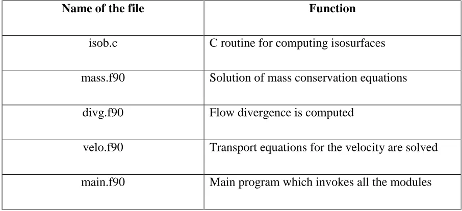
The FDS source code has twenty six FORTRAN files depending on one C file. The twenty six FORTRAN files include one main program and twenty five FORTRAN modules. The C file acts like an external procedure for the source code. The C file is linked to the main program through the twenty five modules. The major files which, we have dealt in the present study are given in the table along with their primary functions.

Table 3.1 – FDS source files and their respective functions

Name of the file Function

isob.c C routine for computing isosurfaces mass.f90 Solution of mass conservation equations

divg.f90 Flow divergence is computed

velo.f90 Transport equations for the velocity are solved main.f90 Main program which invokes all the modules

3.7 Combustion Model in FDS

to the solution of multiple transport equations, for components of the mixture fraction Zβ.

The fuel mass will still be conserved, since ∑Zβ = Z. For example, if Z1 represents the

(unburned) fuel mass fraction, YF, and Z2 = Z –Z1, then, Z2 is the mass fraction of burned fuel

and is the component of Z that originates from the combustion products. Figure 3.2 shows the extinction criteria used in FDS 5 (Mowrer, 2009). This figure represents temperature with oxygen volume fraction. Hence, for combustion to occur, fuel and oxidizer need to mix and reach a particular temperature. However, this flame extinction criterion is not included in our LES-ODT model.

The combustion model, thus, involves consideration of two reactions to consider for any hydrocarbon combustion. They are:

 Null reaction

 Complete reaction

The “null” reaction is the reaction, where fuel and oxygen simply mix and do not burn, the lower left region in figure 3.2, while the “complete” reaction (McGrattan, 2009) is the reaction, where fuel and oxygen react and form products.

Hence, the mixture fractions can be given as in equations (3.33) and (3.34)

1 F I F Y Z Y  (3.33)





2 1 CO F I F

CO H S CO

Y M

Z

Y

x  S  M



  

 

  (3.34)

In the equation (3.24) and (3.25), x is the number of carbon atoms in the fuel, SH is the soot

fraction, 2 CO

Y is the mass fraction of carbon dioxide,_COis the number of moles of carbon monoxide per mole of fuel, _Sis the number of moles of soot formed per mole of fuel, Y_FIis the mass fraction of the fuel at inlet, and YFis the mass fraction of the fuel.

The state relations of fuel and oxygen are given in equation (3.35) and (3.36).

1

I F F

Y Y Z (3.35)





2 1 2 2

O O I

O O F

F M

Y Z Y Y Z

M





The transport equation of the mixture fraction is explained as follows. Consider a simple reaction as follows:

Step 0: F + O2 No Products

Step 1: F + O2 CO + H2O+Soot

Step 2: CO + ½ O2 CO2

The step 0 is called the Null reaction.

Hence, the transport equations for Z1, Z2, Z3 are as given in equations (McGrattan, 2009)

(3.37) - (3.39)

,1 1

1

. F CO

CO M w DZ

D Z

Dt     xM (3.37)

,1 ,2

2

2

. F CO F CO

CO CO

M w M w

DZ

D Z

Dt     xM  xM (3.38)

,2 3

3

. F CO

CO M w DZ

D Z

Dt     xM (3.39)

The molecular weight and production rate for particular species in the equations (3.37) - (3.39) are given by M andw, D denotes the diffusivity, ρ the density and Z1,2,3 denote the

different mixture fractions.

The transport equation of the whole mixture fraction hence is just the addition of the three equations (3.37), (3.38) and (3.39).

.

DZ

D Z Dt

    (3.40)

3.8 Turbulent Viscosity Computation in LES

The viscosity in large eddy simulations is computed using the Smagorinsky Model (1963). The viscosity is given by the equation (3.41).





 

1

2 2

2 2

2 . .

3

LES Cs ij ij

   _   _

 S S u  (3.41)

In the equation (3.41), Cs is an empirical constant, Δ is a length on the order of the size of a

grid cell, ρ is the density, Sijis the symmetric rate of strain tensor, and uis the velocity vector.

The thermal conductivity kLES and material diffusivity DLES are computed from the viscosity,

as shown in equations (3.42) and (3.43).

Pr LES p LES

t C

k   (3.42)

,

( ) LES

l LES t D

Sc



  (3.43)

In the equation (3.42) and (3.43), Sct is the turbulent Schmidt number = 0.7, Prt is the

turbulent Prandtl number = 0.7, Cp is the specific heat, and ρ is the density.

3.9 The Smokeview

in this program including isosurfaces which, we have used in the present study. Some of the other features include slice file, which displays properties at any plane in the domain and smoke3d, which realistically displays the smoke and the fire. The isosurfaces in Smokeview is invoked using the ISOF command in the FDS input file. The isosurfaces can be used to display many flow properties, such as temperature, velocity, mixture fraction, enthalpy, and volume flow. In our present study, the mixture fraction is displayed using the isosurfaces.

3.10 Mean Mixture Fraction Isosurface

3.11 The Marching Cube Algorithm

CHAPTER 4

ODT Formulation and Numerical Implementation

4.1 Objectives

The objective of this chapter is to present the governing equations of the ODT model that are implemented within the context of the LES-ODT approach. Additionally, this chapter also discusses the various processes implemented within the ODT solution.

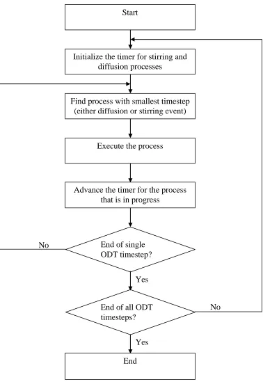
4.2 ODT Model Strategy

Find process with smallest timestep (either diffusion or stirring event)

Start

Execute the process

Advance the timer for the process that is in progress

End of single ODT timestep?

End of all ODT timesteps?

End

Initialize the timer for stirring and diffusion processes

Yes No

Yes

4.3 ODT Governing Equations

The ODT governing equations include transport equations for species, the velocity vector and temperature on the ODT domains.

Equation of Conservation of Species

1 Y Y Y D m t           _     _{  }     

 _ _  _{ } (4.1)

Equations of Conservation of Momentum

1

i

i i

u

u u

t    

 

    

 _{  }  _

 _ _  _{ } (4.2)

Equation of Conservation of Temperature

1

1 1 N

T P

T q

h m

t  c    

    

 _  _{   }

   

 _{ }



The “η” denotes the direction of the ODT domain. In the equations (4.1) - (4.3),Y_,h_, and

m are the species mass fraction, total enthalpy, and production rate for species β, qrepresents the conductive and radiative heat fluxes from a chemical reaction, and

i

 represents the stochastic terms.

The terms inside the brackets “[ ]” include resolved terms such as 1. Diffusion terms

4.4 Scalar Computation in ODT 4.4.1 Viscosity Computation

The viscosity in FDS for Direct Numerical Simulations is computed by the equation (4.4) (Poling, 2000).





7 ₂

2

26.69 *10 v

W T_

       (4.4)

 

1.6145 0.52487 T 2.16178 T

v T e e

 _{ }

    (4.5)

* k

T T



 (4.6)

In equations (4.4) – (4.6), Wβ is the molecular weight of the species β, Ωv is the collision

integral, T is the temperature in the ODT domain and σβ and ε/k are the Lennard Jones

potential parameters of the species β.

1

n

ODT DNS Y 



  



 



In the equation (4.7), Yβ is the mass fraction of the species β, and μβ is the viscosity of the

species β.

4.4.2 Mass Diffusivity and Thermal Conductivity Computation

The mass diffusivity in FDS for Direct Numerical Simulations is computed as follows. We follow the same method to compute it for the One-dimensional Turbulent solutions. The mass diffusivity is directly computed from the temperature as the mesh is finely resolved as shown in equation (4.8). The thermal conductivity is computed in equation (4.13).

3 7 ₂ 1 2 2 2.66 10 D T D W        (4.8) where 2       _{ }  _

  (4.9)

1 1 1 2 W W W        _  _

  (4.10)

 





 





exp exp exp

D B

A C E G

DT FT HT

T

     (4.11)

* AB k T T   

  _{ } (4.12)

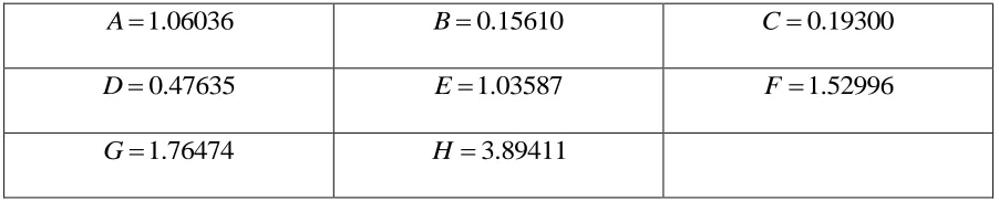
Table 4.1 – Constants used in diffusion collision integral

1.06036

A B0.15610 C0.19300

0.47635

In the equations (4.8) - (4.12), Wαβ is the average molecular weight of the species α and β,

(ε/k)AB and σαβ is the combined Lennard Jones potential parameters of the species α and β, ΩD

is the diffusion collision integral, which, is an empirical function of Temperature as shown in equation (4.11), and T is the temperature.

,

Pr p c k  



 (4.13)

In equation (4.13), _is the viscosity c_p,is the specific heat capacity of species β, and Pr is the turbulent Prandtl number.

4.4.3 Density Computation

The density is computed from the state relation. The thermodynamic pressure is going to be same all through the simulation. Hence, the density is computed using the Ideal Gas relation given in equation (4.14).

P Y RT

W 

 

 



In the equation (4.14), P is the thermodynamic pressure, R is the universal gas constant, T is the temperature, Yβ is the mass fraction of species β and Wβ is the molecular weight of the

The density is directly computed from the mass fraction and temperature, which are being solved in ODT.

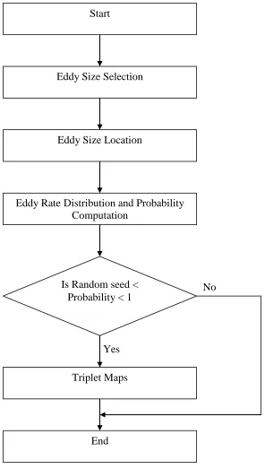
4.5 Stirring Processes in ODT

The procedure adopted here to model turbulent transport, is essentially the same procedure adopted by Kerstein and co-workers (Kerstein et al., 2001), and Cao and Echekki (2008). This procedure is also called “vector ODT” which, transports all the three components of the velocity. The 3D turbulent flow structures are actually captured with 1D line of sight for ODT through the „eddy events‟. This is done by applying a random and instantaneous mapping, called „triplet maps‟, to an interval corresponding to the stirring process. The pressure scrambling model and the derivation to get the amplitudes is shown in the Appendix.

Figure 4.2 – Stirring process in ODT Start

Eddy Size Selection

Eddy Size Location

Eddy Rate Distribution and Probability Computation

Is Random seed < Probability < 1

Triplet Maps

End Yes

min max 2

max min

. 1

( ) s s

f len

s s len

 

 _{ }

   (4.15)

In the equation (4.15), smin is the smallest eddy size, smax is the largest eddy size and len

denotes the eddy length scale. The discrete eddy size is given by equation (4.16).

x

ieds N1d 2

LODT



 

_{ } 

  (4.16)

In the equation (4.16), xis the grid spacing of LES, LODT is the length of a single ODT domain, N1d is the number of ODT grid points in a single ODT domain, and ieds is the discrete eddy size.

The eddy location is selected all along the ODT element. The probability distribution is computed using equation (4.17)





   

; , a

t x len t P

f len g x

 

 (4.17)

In the equation (4.17), tis the timestep between successive eddy events, f(len) and g(x0) are

shapes of probability density function, len denotes the eddy length scale and x0 denotes the

eddy location.

If the probability computed, lies between a random seed and one, then the triplet maps are performed.

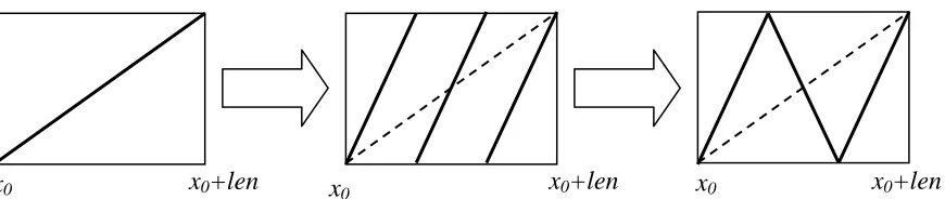
4.5.1 Triplet Mapping

The triplet map is the mapping that emulates the rotational event taking place in an eddy into a single dimension. The triplet map satisfies the conservation equations and hence, the properties remain the same either before or after employing the triplet map. It is given by equation (4.18) (Cao and Echekki, 2008).

3





3

x  x x  len

2len3





3 3

x  len x x  len (4.18) 3





3

x  len x x len

xx₀ otherwise

In the equation (4.18), f(x) is the mapping function, x0 is the starting location of eddy and len

is the length of the eddy.

The mapping clearly is shown in figure 4.3. First, the total line segment is divided into three equal parts. The second part is then inversed, to emulate the rotational effect. This transforms the eddy into triplet maps with the continuity of the function being maintained. The dotted line in figure 4.3 refers to the original eddy.

 

x0

x0 x0+len x0+len x0 x0+len

Figure 4.3 – Triplet mapping

4.5.2 Pressure-Scrambling Model

Wunsch and Kerstein (2001) found out that the triplet mapping of the density affected the total potential energy, when they applied it to buoyant stratified flows. To account for this change in potential energy, they added a kernel transformation function, to add it in the kinetic energy term so that the total energy is conserved. A kernel transformation function K(y) with a prescribed amplitude ci is added to each component of the velocity.

 

 

 

i i i

w y w _f y _c K y (4.19)

In the equation (4.19), ci is the amplitude, K(y) is the kernel transformation function given by

equation (4.20).

 

 

K y  y f y (4.20)

 

, , , ,

27

sgn 4

i i K i K i K ij j K

j

c w w w T w

len 

 

 _   _





In the equation (4.21),  is a free parameter0  1, w is the velocity vector, len is the eddy length scale and T is the transfer matrix given in equation (4.22).

2 1 1

1

1 2 1

2

1 1 2

T       _  _  _    (4.22)

4.6 Molecular Diffusion - Reaction Processes in ODT

The molecular diffusion in ODT for the momentum equations are computed deterministically, through the scalars that are described above. The energy and the species equation of the ODT, have an additional reaction term, other than the diffusion term. This can be seen in equation (4.23) – (4.25).

i i

u 1 u

t    

    

 _{ }

  _  _ (4.23)

N 1 P q T 1 h m t c              _{  }   

 _  _



,

Y 1 J

m t           _  _{ } _

 _  _{ } (4.25)

2

E 5 _RT

f f O

m  B  e (4.26)

2

O f

m  5m (4.27)

In the equations, (4.26) and (4.27), B is a pre-exponential factor, E is the activation energy, R is the universal gas constant, T is the temperature, _fand

2

O

 are the mole fractions of fuel

and oxygen, which can be derived from the mass fractions of fuel and oxygen. The complete combustion of propane involves reaction of five moles of oxygen for each mole of the fuel. Hence, the production rate of oxygen is multiplied by five as shown in equations (4.26) and (4.27). The values of the pre-exponential factor and the activation energy for propane, for stoichiometric value of 0.06, are taken from Puri and Seshadri (1986) as:- . 19

B2 9 10

CHAPTER 5

LES-ODT Formulation and Numerical Implementation

5.1 Objectives

The objective of this chapter is to present the combined LES-ODT formulation and numerical implementation. The previous chapters discussed the LES and ODT separately, while this chapter provides an extension of Chapter 2, by including the solution implementation.

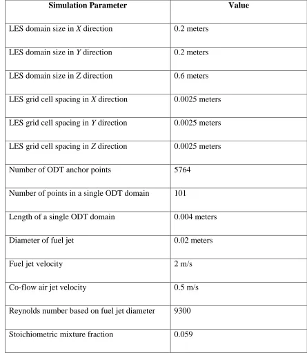
5.2 Simulation Conditions

Table 5.1 : Simulation Conditions

Simulation Parameter Value

LES domain size in X direction 0.2 meters LES domain size in Y direction 0.2 meters LES domain size in Z direction 0.6 meters LES grid cell spacing in X direction 0.0025 meters LES grid cell spacing in Y direction 0.0025 meters LES grid cell spacing in Z direction 0.0025 meters Number of ODT anchor points 5764

Number of points in a single ODT domain 101

Length of a single ODT domain 0.004 meters

Diameter of fuel jet 0.02 meters

Fuel jet velocity 2 m/s

Co-flow air jet velocity 0.5 m/s Reynolds number based on fuel jet diameter 9300

5.3 Schematics of ODT domain

The ODT anchor points are the points, where the ODT domains are attached. In figure 5.1, consider the red line to be the flame brush in two dimensions. The black dotted lines attached to the red line, represent the ODT domains in the flame brush. The intersection of the black lines and the red line provides the ODT anchor points. The ODT domains are locally normal to the flame surface and each ODT domain is of a constant length prescribed by us. The number of ODT domains can be either increased, or decreased depending upon the resolution needed. This is usually denoted as „Num1d‟. Each of the black lines will have certain number of points which, again is prescribed by us. We usually consider an odd number of grid points so that the anchor point forms the midpoint with equal points on its either side. This is denoted as „N1d‟. The flow variables in ODT hence, will be dependent on these two variables, „Num1d‟ and „N1d‟.

Figure 5.1 – Schematics of ODT domain ODT domain Stoichiometric mixture fraction surface

5.4 Minimum and Maximum Positions of ODT domains

The minimum and maximum position of the ODT domain, in each anchor point, needs to be calculated for interpolation of flow variables in one dimension. The minimum and maximum positions are computed with the help of the midpoint (anchor point) and the normals (direction of ODT solution) as shown in the equation (5.1).

1 1 . . 2

i c

N d

X X  _i _  _n

 

  (5.1)

1 1

L N d



 

 (5.2)

1 i N1d (5.3)

In the equations (5.1), (5.2), and (5.3), N1d is the number of ODT points in a single ODT domain placed at a single anchor point, i refers to any point along the ODT domain, L is the length of the ODT domain,X_cdenotes the coordinates of the anchor point and X_idenotes the coordinates of all the points in a single ODT domain. After all the points in a single ODT domain are computed, the minimum and maximum points in each ODT domain are computed.

5.5 The Flame Displacement Speed Derivation





.

j j j

j j j j

Z Z Z

u D u Z u Z

t x x x x

 

    

  _ _ 

   _  _  (5.4)

In the equation (5.4), D is the mass diffusivity and u Z_j is the combined Favre averaging of velocity uj with mixture fraction Z.

Favre averaging of any quantity φ is given by equation (5.5),

 



 (5.5)

In FDS, the last term of equation (5.4) is computed as given by equation (5.6),





j j t j

Z u Z u Z

x x Sc x



 

  

  _ _

  _  _ (5.6)

In the equation (5.6), ν is the kinematic viscosity, Sct is the turbulent Schmidt number.

Also, the total derivative or the material derivative of the mixture fraction is zero as given by equation (5.7).

0 j.

j dx

DZ Z Z

Dt t dt x

 

  

  (5.7)

The dxj

dt term in equation (5.7) is a summation of the velocity and the scalar flame displacement speed Sd.

j

j d j dx

u S n

dt   (5.8)

Substituting equation (5.8) in equation (5.7), we get equation (5.9).

Z Z Z

Substituting equation (5.9) and equation (5.6) in the main transport equation, equation (5.4), we get equation (5.10),

d j

j j j j t j

Z Z Z

S n D

x x x x Sc x



   

    

  _ _ _ _

  _  _  _  _ (5.10)

. t d D Z Sc S Z                  (5.11)

Hence, the flame displacement speed is computed by the equation (5.11).

The flame displacement speed needs to be interpolated to the anchor points after being computed all through the domain. This is done by the tri-linear interpolation technique as discussed in section 5.6. The anchor points are updated as shown in equation (5.12).

j

j d j dx

u S n

dt   (5.12)

Z n Z    (5.13)

5.6 Flow Variables Initialization for ODT 5.6.1 Temperature and Mass fractions

The temperature (T), mass fraction of oxidizer (Yo), and the mass fraction of fuel (Yf) are all

Table 5.2 : Scalar initialization from LES mixture fraction

Cases Scalar Variable Boundary

Conditions Linear Function

Surface above the flame

surface st Z Z

Temperature, T aZb

0, _u

Z  T T

, st b Z Z TT

b u

u st

T T

T Z T

Z

  

_{ } 

 

Mass fraction of Oxygen, O

Y aZb

0, _O 1 Z  Y 

, 0

st O Z Z Y 

1 O st Z Y Z  

Mass fraction of Fuel, F

Y aZb

0, _F 0 Z  Y 

1, _F 0

Z  Y 

0

F Y 

Surface below the flame

surface st Z Z

Temperature, T aZb

, st b Z Z TT

1, _u Z  T T





1

b u u st b

st

T T Z T Z T

T Z        _   

Mass fraction of Oxygen, O

Y aZb

0, O 0 Z  Y 

1, _O 0 Z  Y 

0

O Y 

Mass fraction of Fuel, F

Y aZb

1, _F 1 Z  Y 

, 0

st F

Z Z Y  1

arbitrary constants. The plots of the temperature and mass fractions with Z are shown in figure 5.2 and figure 5.3.

Figure 5.2 – Temperature initialization

Figure 5.3 –Mass fractions initialization

5.6.2 Velocity

5.7 Interpolation

The interpolation used in our case is a tri-linear interpolation, which is similar to bilinear interpolation (Press, 1996). The tri-linear interpolation is done as follows. The parameter, which needs to be interpolated, is first computed over the entire domain. For a variable, B, defined over the entire domain the interpolation is implemented as follows. The three dimensional field variable B is prescribed as an array in discrete Cartesian coordinates given by B (i,j,k) where, i ranges from 0 to ibar, j ranges from 0 to jbar and k ranges from 0 to kbar. The variables ibar, jbar, and, kbar denote the maximum integer given by following equations (5.14) – (5.16).

max min

int x x

ibar x     _{ } 

  (5.14)

max min

int y y jbar

y

  

 _{ }



  (5.15)

max min

int z z

kbar z     _{ } 

  (5.16)

In the equation (5.14) – (5.16), Δx, Δy and Δz denote the dimensions of a single grid cell in x, y, and z directions respectively, xmin, xmax, ymin, ymax, zmin and zmax denote the minimum and

maximum points of the domain in x, y and z directions respectively.

and z directions respectively, as scalars are computed at cell centers. Then the distance of the point (xi,yi,zi) is computed from the minimum x, y and z coordinate of the grid cell which

contains the point. These are correspondingly denoted by α, β and γ as shown in equations (5.17) - (5.19). Then the interpolation is given by equation (5.20).

min

i

x x

x

 _{ }  _



  (5.17)

min

i y y

y

 _{ }  _



  (5.18)

min

i

z z

z

 _{ }  _



  (5.19)

B = (1 - α) (1 - β) (1 – γ) Bi,j,k

+ (1 - α) (1 - β) ( γ) Bi,j,k+1

+ (1 - α) ( β) (1 - γ) Bi,j+1,k

+ (1 - α) ( β) ( γ) Bi,j+1,k+1

+ ( α) (1 - β) (1 - γ) Bi+1,j,k (5.20)

+ ( α) ( β) (1 - γ) Bi+1,j+1,k

+ ( α) (1 - β) ( γ) Bi+1,j,k+1

Figure 5.4 – Interpolation of a field variable B (x,y,z) β

α

i-direction

k-direction

B (x,y,z) α

γ

i-direction j-direction

k-direction

Ai+1,j+1,k+1

Ai,j+1,k

Ai+1,j,k+1

Ai,j,k+1 Ai+1,j,k+1

Ai+1,j+1,k

Ai+1,j,k

j-direction

5.8 Filtering Operation

The filtering is the inverse operation of interpolation process. The filtering process is added primarily to transfer the interpolated flow variables in one dimension back to three dimensions. This operation is also included so as to capture the fluctuations in the velocity field. Hence, this filtering process occurs, when the LES timestep is incremented and ODT process is started. The filtering operation is given by equation (5.21).

 

  



h y 



In the equation (5.21), ( )h y is the filtered flow variable, h y( ) is the original flow variable and L is the filter function satisfying equation (5.22).

 



In this present study, we have used the box filter, though there are many types of filters. The

box filter for an interval of y 1 y y 1

2  2

     is given by equation (5.23).

 

,

,

0 y y 2 1

y y

2

 

 

 

 



CHAPTER 6 Results and Conclusions

6.1Objectives

The objective of this chapter is to present the results obtained, after implementing the LES-ODT approach. This chapter also provides the conclusions of this novel approach implemented along with the FDS code. The last part of this chapter includes the recommendations for future work.

6.2 Outputs of the Simulations in Smokeview

Time 0.62 seconds

Time 0.67 seconds

6.3 Mixture Fraction during the Simulation

Figure 6.2 shows the plot of mixture fraction at a single anchor point with respect to the time. The mixture fraction value is the stoichiometric value at most of the time. This ensures that our ODT domains stay attached to the flame brush. Though, the mixture fraction need not be calculated at each timestep to generate temperature and mass fractions, as done for the initial ODT step, this plot is to verify that the ODT domains are attached to the flame brush.