Modeling Epistasis of Quantitative Trait Loci Using Cockerham’s Model
Chen-Hung Kao* and Zhao-Bang Zeng
†*Institute of Statistical Science, Academia Sinica, Taipei 11529, Taiwan, Republic of China and†Bioinformatics Research Center,
Departments of Statistics and Genetics, North Carolina State University, Raleigh, North Carolina 27695-7566 Manuscript received May 10, 2001
Accepted for publication January 9, 2002
ABSTRACT
We use the orthogonal contrast scales proposed by Cockerham to construct a genetic model, called Cockerham’s model, for studying epistasis between genes. The properties of Cockerham’s model in modeling and mapping epistatic genes under linkage equilibrium and disequilibrium are investigated and discussed. Because of its orthogonal property, Cockerham’s model has several advantages in partitioning genetic variance into components, interpreting and estimating gene effects, and application to quantitative trait loci (QTL) mapping when compared to other models, and thus it can facilitate the study of epistasis between genes and be readily used in QTL mapping. The issues of QTL mapping with epistasis are also addressed. Real and simulated examples are used to illustrate Cockerham’s model, compare different models, and map for epistatic QTL. Finally, we extend Cockerham’s model to multiple loci and discuss its applications to QTL mapping.
G
ENES interact when they express their effects;i.e., components corresponding to additive, dominance, the effects of genotypes at one locus depend on and epistatic variances using the least-squares princi-what genotypes are present at other loci. Interaction ple. Cockerham (1954) further partitioned the epi-(epistasis) between genes affecting qualitative trait varia- static variance into components using orthogonal con-tion has been demonstrated for a long time since Gregor trasts. Kempthone (1957) and Haymanand MatherMendel in 1865. Although the evidence of epistasis be- (1955) adopted the same epistasis model.Haymanand tween genes controlling quantitative traits [quantitative Mather (1955) and Mather (1967) proposed other trait loci (QTL)] has been reported by traditional tech- epistasis models for modeling epistasis.Van Der Veen
niques, such as variance component analyses (Brimand (1959) reviewed the genetic models of digenic epistasis
Cockerham1961; Lee et al. 1968;Stuber andMoll published by then and summarized them into three 1971), epistasis between individual QTL generally has categories:
been difficult to discern by traditional techniques. The
a. The pure-line-metric orF∞-metric model (F∞denotes
recent advances in molecular biology have allowed
fine-the population derived from selfing F2 individuals scale genetic marker maps of various organisms to be
for tgenerations as t →∞): The parameters in the constructed for the study of individual QTL. Using such
F∞-metric model show orthogonality with respect to
maps, statistical methods for estimating the positions and
genotypic frequencies of anF∞population under
link-effects of individual QTL (QTL mapping) have been
age equilibrium. proposed (Lander andBotstein 1989; Jansen 1993;
b. TheF2-metric model (corresponding to Cockerham’s
Zeng1994;Kaoet al.1999;SenandChurchill2001).
model): The parameters in theF2-metric model are The problem of epistasis has been considered in some
mutually orthogonal with respect to genotypic fre-QTL mapping studies (e.g., Stuber et al.1992;
Cheve-quencies of an F2population under linkage
equilib-rudandRoutman1995;Doebleyet al.1995;
Cocker-rium.
hamandZeng1996;Kaoet al.1999;Goodnight2000;
c. The mixed-metric model (corresponding to Hayman
Zenget al.2000), but not sufficiently, and many
theoreti-and Mather’s model): The mixed-metric model is a cal and statistical issues involved with epistasis have not
mixture of the Cockerham’s model and F∞-metric
been discussed. Here, we discuss a genetic model, called
model, and it can be transformed to the F2-metric Cockerham’s model, in relation to QTL mapping with
model by subtraction of the mean. epistasis. We also investigate the model properties under
linkage disequilibrium.
Later, Crow and Kimura (1970), Mather and Jinks Fisher (1918) first partitioned genetic variance into
(1982), Haley andKnott (1992), and Kearsey and
Pooni(1996) applied theF∞-metric model to the study
of epistasis between genes, and Goodnight (2000) Corresponding author :Institute of Statistical Science, Academia
Sin-adopted an alternative model modified from
Cocker-ica, Taipei 11529, Taiwan, Republic of China.
E-mail: [email protected] ham(1954) to study gene interaction. Although these
three models can be translated to each other by addition the scale component of genotypeijfor thetth contrast. The first requirement ensures that deviations around or subtraction of a constant (see Table 1 of Van Der
Veen’s 1959 article), they have different meanings in the mean are compared (the scalesWtij’s are contrasts).
The second requirement ensures that the contrasts are interpreting gene effects, show different structures of
variance components, and possess different properties orthogonal.W1andW2(W3andW4) are the linear and quadratic orthogonal contrasts for locus A (locus B). in statistical estimation, which may affect the study of
W5 is the linear ⫻ linear contrast. W6 is the linear ⫻ QTL as shown in this article.
quadratic contrast.W7is the quadratic⫻linear contrast. In this article, we start from the traditional partition
W8is the quadratic⫻ quadratic contrast. Cockerham’s of genetic variance into variance components using
orthogonal contrast scales serve the same purpose as
Cockerham’s (1954) orthogonal contrasts, then lead
the orthogonal contrasts for partitioning the sum of up to a definition of the genetic parameters for genetic
squares due to treatment into independent single-effects, and present Cockerham’s epistasis model. The
degree-of-freedom components in experimental design properties of Cockerham’s model in modeling and
map-(Steel and Torrie 1981). The statistical linear and ping epistatic genes are investigated when genes are in
quadratic terms correspond to the genetical additive linkage equilibrium and disequilibrium. The
differ-and dominance terms, respectively. Cockerham used ences between Cockerham’s model and the other
mod-these orthogonal scales to partition the genetic variance els are compared, and the advantages of Cockerham’s
and find the partition of variance2
t due to orthogonal
model are discussed. It shows that Cockerham’s model
scaleWtby
is a more appropriate model than the other models for the study of epistasis between genes and QTL mapping
2
t ⫽
(兺i,jpijGijWtij)2
(兺i,jpijW2tij)
, in the populations, such as F2and backcross. Real and
simulated examples are used to illustrate Cockerham’s
model, compare different genetic models in the analysis where Gijdenotes the genotypic value of the genotype
of epistasis between genes, and map for epistatic QTL. ij.He also definedGijin terms of the scales as
Finally, we generalize Cockerham’s model to multiple
Gij ⫽E0⫹
兺
8t⫽1
EtWtij, (1)
loci and discuss its applications to QTL mapping.
whereEt’s are the corresponding coefficients, by solving
COCKERHAM’S GENETIC MODEL the equations themselves, and used it to find the
correla-tion between relatives in a populacorrela-tion. His idea of
defin-Cockerham (1954) used eight orthogonal contrast
ing the genotypic value by the orthogonal contrast scales scales to partition the genetic variance contributed by
leads up to Cockerham’s genetic model for modeling two genes into eight components and to define the
ge-epistasis between genes. notypic value of a genotype to find the correlation
be-Cockerham’s genetic model: We now apply Cocker-tween relatives in a population. His definition of
geno-ham’s orthogonal contrast scales to the F2 population typic value using the orthogonal scales leads the way to
to derive Cockerham’s model for the F2population. For construct a genetic model, which is called Cockerham’s
an F2population, the genotypic frequencies of the nine model, for modeling epistasis and defining gene effects
genotypesAABB,AABb,AAbb,AaBB,AaBb,Aabb,aaBB, in a population. In this section, the orthogonal contrast
aaBb, andaabbare 1/16, 1/8, 1/16, 1/8, 1/4, 1/8, 1/16, scales are introduced to present Cockerham’s model,
1/8, and 1/16, respectively, and Cockerham’s orthogo-and the genetic parameters of Cockerham’s model are
nal contrasts can be modified as shown in Table 1 (see defined. The similarities and differences between
Cock-also Cockerham and Zeng 1996). By solving Equa-erham’s model and alternative models are compared,
tion 1 with the scales in Table 1, the unique solutions and their variance component structures are presented.
of the coefficients in terms of the genotypic values are
Orthogonal contrasts: Assuming that allele frequen-cies at one locus are uncorrelated with frequenfrequen-cies at
E0⫽ G22
16 ⫹ G21
8 ⫹ G20
16 ⫹ G12
8 ⫹ G11
4 another locus (two loci are in linkage equilibrium),
Cockerham (1954) partitioned the genetic variance
caused by two loci, A and B, each with two alleles (A, ⫹ G10 8 ⫹
G02 16 ⫹
G01 8 ⫹
G00
16, (2)
a, andB,b), of a diploid organism using the orthogonal contrast scales in Table 2 of his article. The scales
E1⫽G22 8 ⫹
G21 4 ⫹
G20 8 ⫺
G02 8 ⫺
G01 4 ⫺
G00
8 , (3) W⬘t’s, which are functions of genotypic frequenciespij’s,
have to satisfy two requirements
E2⫽ G12
8 ⫹ G11
4 ⫹ G10
8 ⫺ G22
16 ⫺ G21
8
兺
i,jpijWtij⫽0 and兺
i,j
pijWtijWt⬘ij ⫽0,
wherei(j) indexed by 2, 1, or 0 refers to the genotype ⫺ G20 16 ⫺
G02 16 ⫺
G01 8 ⫺
G00 16
, (4)
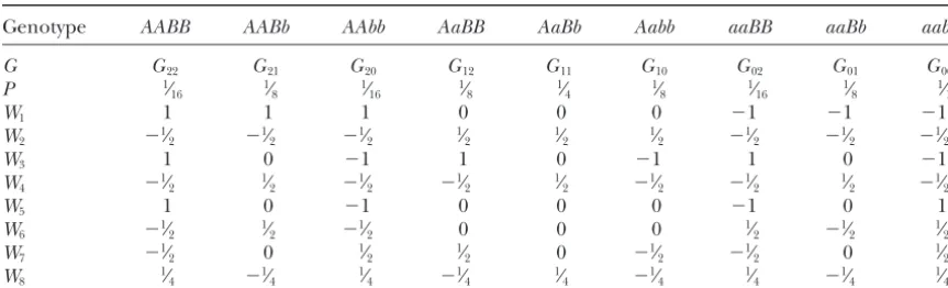
TABLE 1
The eight orthogonal contrast scales (W’s) for the F2population
Genotype AABB AABb AAbb AaBB AaBb Aabb aaBB aaBb aabb
G G22 G21 G20 G12 G11 G10 G02 G01 G00
P 1⁄
16 1⁄8 1⁄16 1⁄8 1⁄4 1⁄8 1⁄16 1⁄8 1⁄16
W1 1 1 1 0 0 0 ⫺1 ⫺1 ⫺1
W2 ⫺1⁄2 ⫺1⁄2 ⫺1⁄2 1⁄2 1⁄2 1⁄2 ⫺1⁄2 ⫺1⁄2 ⫺1⁄2
W3 1 0 ⫺1 1 0 ⫺1 1 0 ⫺1
W4 ⫺1⁄2 1⁄2 ⫺1⁄2 ⫺1⁄2 1⁄2 ⫺1⁄2 ⫺1⁄2 1⁄2 ⫺1⁄2
W5 1 0 ⫺1 0 0 0 ⫺1 0 1
W6 ⫺1⁄2 1⁄2 ⫺1⁄2 0 0 0 1⁄2 ⫺1⁄2 1⁄2
W7 ⫺1⁄2 0 1⁄2 1⁄2 0 ⫺1⁄2 ⫺1⁄2 0 1⁄2
W8 1⁄4 ⫺1⁄4 1⁄4 ⫺1⁄4 1⁄4 ⫺1⁄4 1⁄4 ⫺1⁄4 1⁄4
G’s andP’s denote the genotypic values and expected genotypic frequencies for the nine genotypes of two
unlinked genes, A and B.
AAandaaand thus is defined as the genetic parameter of dominance effect of geneA,d1. The same argument E3 ⫽G22
8 ⫹ G12
4 ⫹ G02
8 ⫺ G20
8 ⫺ G10
4 ⫺ G00
8 , (5) leads us to define coefficientsE
3andE4as the genetic parameters of additive and dominance effects of gene E4 ⫽
G21 8 ⫹
G11 4 ⫹
G01 8 ⫺
G22 16 ⫺
G12
8 B, a2 and d2. If the substitution effects at one locus depend on genotypes at the other locus, there is an interaction between the two genes in the usual sense.
⫺G02 16 ⫺
G20 16 ⫺
G10 8 ⫺
G00
16, (6) CoefficientE5 quantifies the difference between addi-tive effects of gene A (gene B), (G2*⫺ G0*)/2 [(G*2⫺ E5 ⫽(G22⫺G02)⫺(G20⫺G00)
4 G*0gotes of gene B (gene A),)/2], in the background of two different homozy-BBandbb(AAandaa), and
this difference is defined as the genetic parameter of
⫽(G22⫺G20)⫺(G02⫺G00)
4 , (7) additive ⫻ additive epistatic effect, iaa. The larger the
difference is, the stronger the interaction is. The same argument leads to the definitions ofE6,E7, andE8 as E6 ⫽(2G21⫺ G22⫺G20)⫺(2G01⫺G02⫺G00)
4
, (8)
the genetic parameters of additive ⫻ dominance, iad;
dominance ⫻ additive, ida; and dominance ⫻
domi-E7 ⫽(2G12⫺ G22⫺G02)⫺(2G10⫺G20⫺G00)
4 , (9) nance,idd; epistatic effects between genes A and B. The definitions of these nine genetic parameters are summa-rized in Table 2. After defining the genetic parameters E8 ⫽2(2G11⫺G21⫺G01)⫺(2G12⫺ G22⫺G02)
4 of genetic effects, Equation 1 can be expressed more succinctly as
⫺(2G10⫺G20⫺ G00)
4 Gij⫽ ⫹a1x1⫹ d1z1⫹a2x2 ⫹d2z2⫹ iaawaa⫹iadwad
⫹idawda⫹ iddwdd, (11)
⫽2(2G11⫺ G12⫺G10)⫺(2G21⫺ G22⫺G20)
4 by defining the coded variables as
⫺(2G01⫺G02⫺ G00)
4 . (10)
x1⫽
冦
1 if A isAA 0 if A isAa
⫺1 if A isaa,
x2⫽
冦
1 if B isBB 0 if B isBb
⫺1 if B isbb, If the two genes are in linkage equilibrium, E0 is the
mean of the genotypic values,G.., and therefore can be denoted as . Coefficient E1 is equivalent to (G2. ⫺
z1⫽
冦
1⁄2 if A isAa
⫺1⁄
2 otherwise ,
z2⫽
冦
1⁄2 if B isBb
⫺1⁄
2 otherwise , G0.)/2, which is one-half of the difference in genotypic
value between the two homozygote means ofAAandaa
waa⫽x1⫻ x2, wad⫽ x1⫻z2, wda⫽ z1⫻x2, and thus is defined as the genetic parameter of additive
effects of gene A, a1. Coefficient E2 is equivalent to w
dd⫽z1⫻z2. (2G1. ⫺ G2. ⫺ G0.)/2, which represents the departure
The coded variables of this model are mutually indepen-in genotypic value of the heterozygote mean ofAafrom
TABLE 2 tion, the structure of variance components for the total genetic variance,VG, contributed by the two genes, each
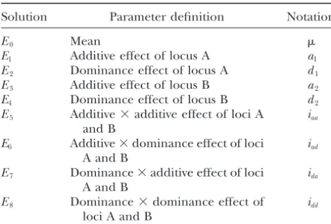
Definition of genetic parameters
with two alleles, is shown inappendix c.Fromappendix c, we can see that the total genetic variance is
com-Solution Parameter definition Notation
posed of genetic variance of individual effects and
co-E0 Mean variances between different effects, and it will change
E1 Additive effect of locus A a1
with gene frequencies (p’s) and linkage disequilibrium
E2 Dominance effect of locus A d1
(D). Certainly, the relative strengths of genetic effects
E3 Additive effect of locus B a2
will vary according to the change in gene frequency and
E4 Dominance effect of locus B d2
E5 Additive⫻additive effect of loci A iaa linkage disequilibrium. For an F2 population (pA⫽pB⫽
and B 0.5), the total genetic variance reduces to Equation 34
E6 Additive⫻dominance effect of loci iad and contains covariances between different genetic
ef-A and B fects through linkage. If genes are unlinked in the F
2
E7 Dominance⫻additive effect of loci ida
population (pA⫽pB⫽0.5 andD⫽0), the total genetic
A and B
variance can be partitioned into eight independent
E8 Dominance⫻dominance effect of idd
components without covariance as
loci A and B
Ei’s are the solutions of Equation 1 with the orthogonal V
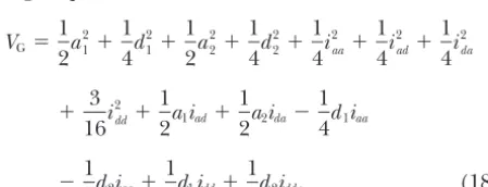
G⫽ 1 2a 2 1⫹ 1 4d 2 1⫹ 1 2a 2 2⫹ 1 4d 2 2⫹ 1 4i 2 aa⫹ 1 8i 2 ad⫹ 1 8i 2 da⫹ 1 16i 2 dd.
contrast scales in Table 2. The exact expressions ofEi’s are
shown in Equations 2–10. (12)
Each variance component is contributed by its own ge-can also be represented in a different form as Table 3. netic parameter. For example, the additive variance Note that the marginal means of the three genotypes, component of gene A,a21/2, is contributed by its additive G2., G1., andG0., for locus A are ⫹ a1 ⫺ d1/2, ⫹ effect, a1, and it has no genetic covariance with other d1/2, and ⫺a1⫺d1/2, respectively, as the segregation effects. This property greatly facilitates the evaluation ratio is 1:2:1. There are similar forms for locus B. The of the contribution of an effect to the genetic variance. grand meanG..is equivalent to. The other models, such asF∞-metric and mixed-metric Genetic variance structure: When applying Cocker- models, do not have such a property (see Equation 18).
Linkage disequilibrium:The coded variables in Cocker-ham’s model to modeling genotypic values in a
popula-TABLE 3
Cockerham’s model (theF2-metric model)
AA Aa aa
G22 G12 G02 G.2
BB ⫹
a1⫺
d1
2 ⫹a2⫺
d2
2 ⫹
d1
2 ⫹a2⫺
d2
2 ⫺a1⫺
d1
2 ⫹a2⫺
d2
2 ⫹a2⫺
d2
2 ⫹iaa⫺
iad 2 ⫺ ida 2 ⫹ idd 4 ⫹ ida 2 ⫺ idd
4 ⫺iaa⫹
iad 2 ⫺ ida 2 ⫹ idd 4
G21 G11 G01 G.1
Bb ⫹
a1⫺
d1
2 ⫹
d2
2 ⫹
d1
2 ⫹
d2
2 ⫺a1⫺
d1
2 ⫹
d2
2 ⫹
d2
2 ⫹iad
2 ⫺ idd 4 ⫹ idd 4 ⫺ iad 2 ⫺ idd 4
G20 G10 G00 G.0
bb ⫹
a1⫺
d1
2 ⫺a2⫺
d2
2 ⫹
d1
2 ⫺a2⫺
d2
2 ⫺a1⫺
d1
2 ⫺a2⫺
d2
2 ⫺a2⫺
d2
2 ⫺iaa⫺
iad 2 ⫹ ida 2 ⫹ idd 4 ⫺ ida 2 ⫺ idd
4 ⫹iaa⫹
iad 2 ⫹ ida 2 ⫹ idd 4
G2. G1. G0. G..
⫹a1⫺
d1
2 ⫹
d1
2 ⫺a1⫺
d1
2
The marginal meansGi.(G.j) for locus A (B) are calculated under segregation ratio 1:2:1 forAA(BB),Aa
(Bb), andaa(bb) in the F2population. The genetic parametersa1,d1,a2,d2,iaa,iad,ida, andiddare defined in
TABLE 4
TheF∞-metric model
AA Aa aa
G22 G12 G02 G.2
BB ⫹a1⫹a2⫹iaa ⫹d1⫹a2⫹ida ⫺a1⫹a2⫺iaa ⫹a2⫹
d1
2 ⫹
ida
2
G21 G11 G01 G.1
Bb ⫹a1⫹d2⫹iad ⫹d1⫹d2⫹idd ⫺a1⫹d2⫺iad ⫹
d1
2 ⫹d2⫹
idd
2
G20 G10 G00 G.0
bb ⫹a1⫺a2⫺iaa ⫹d1⫺a2⫺ida ⫺a1⫺a2⫹iaa ⫹
d1
2 ⫺a2⫺
ida
2
G2. G1. G0. G..
⫹a1⫹
d2
2 ⫹
iad
2 ⫹d1⫹
d2
2 ⫹
idd
2 ⫺a1⫹
d2
2 ⫺
iad
2 ⫹
d1
2 ⫹
d2
2 ⫹
idd
4
The marginal meansGi.(G.j) for locus A (B) are calculated under segregation ratio 1:2:1 forAA(BB),Aa
(Bb), andaa(bb).a1(a2) andd1(d2) are the additive and dominance effects of locus A (B).iaa, iad, ida, and
idd are the additive-by-additive, additive-by-dominance, dominance-by-additive, and dominance-by-dominance
epistatic effects.
ham’s model (the scales in Table 1) are orthogonal and between the two homozygotes is not equal to the genetic parameter of additive effecta1(a2). For example,G2.⫽ contrast to each other when the ratio of genotypic
fre-quencies is 1:2:1:2:4:2:1:2:1 (genes are unlinked) in an ( ⫹a1⫹d2/2 ⫹iad/2), (G2.⫺ G0.)⫽ a1⫹iad/2, and
G.. ⫽ ⫹ d1/2 ⫹ d2/2 ⫹ idd/4 (Table 4). This result
F2population. Therefore, the definition of the genetic
parameters in Table 2 is appropriate for interpreting the deviates from the usual definition in the one-locus analy-sis. The solutions of the marginal genetic parameters, gene effects and the genetic variance can be partitioned
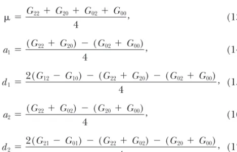
(Equation 12) as if genes are unlinked. If there is seg- a1,d1,a2,d2, in terms of the genotypic values for the F∞-metric model are
regation distortion and/or linkage, the ratio will deviate from 1:2:1:2:4:2:1:2:1 (Table 6) and there will be
covari-ances between some genetic effects (Equation 34). To take ⫽G22⫹G20⫹G02⫹G00
4 , (13)
linkage disequilibrium into account in using Cocker-ham’s model, we introduce statistical parameters to
con-a1 ⫽(G22⫹G20)⫺(G02⫹G00)
4 , (14)
trast with genetic parameters in interpreting gene ef-fects when genes are in linkage disequilibrium (see next
section). d1 ⫽2(G12⫺ G10)⫺ (G22⫹ G20)⫺ (G02⫹G00)
4 , (15)
F∞-metric and mixed-metric models:TheF∞-metric model
can be expressed in equation form as Equation 11 by
a2 ⫽(G22⫹G02)⫺(G20⫹G00)
4 , (16)
coding
d2 ⫽
2(G21⫺ G01)⫺ (G22⫹ G02)⫺ (G20⫹G00)
4 , (17)
x1⫽
冦
1 if A is AA 0 if A is Aa
⫺1 if A is aa,
x2⫽
冦
1 if B isBB 0 if B isBb
⫺1 if B isbb,
and the solutions of epistasis genetic parameters,iaa,iad,
ida, andidd, are the same as those in Cockerham’s model.
z1⫽
冦
1 if A isAa0 otherwise , z2⫽
冦
1 if B isBb
0 otherwise , Apparently, most of the heterozygotes are excluded in the estimation ofand marginal parameters, making andwaa ⫽ x1 ⫻ x2, wad ⫽ x1 ⫻ z2,wda ⫽ z1 ⫻ x2, and the F∞-metric model difficult in interpreting the gene
wdd ⫽ z1 ⫻ z2, where the coded variables for epistasis action for the F2population.
are just the products of marginal variables. Equivalently, The equation form for the mixed-metric model, which theF∞-metric model can be illustrated by Table 4. It is is a mixture of Cockerham’s model and theF∞-metric
easy to check that the coded variables of theF∞-metric model with the first part of marginal effects from the
model do not have the property of orthogonal contrast. F∞-metric model and the latter part of epistatic effects
TABLE 5
The mixed-metric model
AA Aa aa
G22 G12 G02 G.2
BB ⫹a1⫹a2 ⫹d1⫹a2 ⫺a1⫹a2 ⫹
a2⫹
d1
2 ⫹iaa⫺
iad
2 ⫺
ida
2 ⫹
idd
4 ⫹
ida
2 ⫺
idd
4 ⫺iaa⫹
iad
2 ⫺
ida
2 ⫹
idd
4
G21 G11 G01 G.1
Bb ⫹a1⫹d2 ⫹d1⫹d2 ⫹a1⫹d2 ⫹
d2⫹
d1
2 ⫹iad
2 ⫺
idd
4 ⫹
idd
4 ⫺
iad
2 ⫺
idd
4
G20 G10 G00 G.0
bb ⫹a1⫺a2 ⫹d1⫺a2 ⫺a1⫺a2 ⫺
a2⫹
d1
2 ⫺iaa⫺
iad
2 ⫹
ida
2 ⫹
idd
4 ⫺
ida
2 ⫺
idd
4 ⫹iaa⫹
iad
2 ⫹
iad
2 ⫹
idd
4
G2. G1. G0. G..
⫹a1⫹
d2
2 ⫹d1⫹
d2
2 ⫺a1⫹
d2
2 ⫹
d1
2 ⫹
d2
2
The marginal means Gi.(G.j) for loci A (B) are calculated under segregation ratio 1:2:1 forAA (BB),Aa
(Bb), and aa(bb).a1(a2) andd1(d2) are the additive and dominance effects of locus A (B).iaa,iad,ida, and
iddare the additive-by-additive, additive-by-dominance, dominance-by-additive, and dominance-by-dominance
epistatic effects.
MODELING QUANTITATIVE TRAITS
for , the solutions of the genetic parameters of the
mixed-metric model are the same as those of Cocker- When applying Cockerham’s model to analyze a quanti-ham’s model. The solution of is not equal toG... By tative trait, controlled by two epistatic genes A and B, subtractingd1/2 ⫹ d2/2, the mixed-metric model will from a sample of size n of an F2 population, the trait become Cockerham’s model. In Table 5, the marginal value of thekth individual with genotypeijcan be mod-means of one locus involve the dominance effect of eled as
another locus, which deviates from the one-locus
analy-yijk⫽Gij⫹εijk
sis. For example, the marginal mean of genotype AA,
G2., is ⫹a1⫹d2/2. Except for, the solutions of the ⫽ ⫹a1x1⫹d1z1⫹a2x2 ⫹d2z2⫹ iaawaa
genetic parameters of the mixed-metric model are the
⫹iadwad⫹ idawda⫹iddwdd⫹εijk, (19)
same as those of Cockerham’s model.
As the F∞-metric model is not an orthogonal model, whereεijkis a residual. LetP˜ijandnijdenote the observed
the total genetic variance contributed by two genes in frequency and sample size of genotypeij where nij ⫽ linkage equilibrium is n ⫻ P˜ij. In expectation,E(nij) ⫽ n ⫻ Pij and E(yij.)⫽ n ⫻ Pij ⫻ Gij, wherePij is the population frequency of
VG⫽ 1 2a
2 1⫹
1 4d
2 1⫹
1 2a
2 2 ⫹
1 4d
2 2⫹
1 4i
2
aa⫹
1 4i
2
ad ⫹
1 4i
2
da genotype ij and depends on the linkage strength
be-tween genes (Table 6). Note that the ratio of Pij’s
re-duces to 1:2:1:2:4:2:1:2:1 if genes are unlinked (D⫽0).
⫹ 3
16i 2
dd⫹
1 2a1iad⫹
1 2a2ida⫺
1
4d1iaa Least-squares estimates of genetic parameters: The least-squares estimates (LSE) of the genetic parameters in Equation (19) have similar formulations as those of
⫺ 1
4d2iaa⫹ 1 4d1idd⫹
1
4d2idd, (18) Equations 2–10 except thatGijis replaced withyij.. For example, the LSE ofa1is
which consists of the covariances between marginal and epistatic gene effects. These covariances make the
evalu-aˆ1⫽ y22.
8 ⫹ y21.
4 ⫹ y20.
8 ⫺ y02.
8 ⫺ y01.
4 ⫺ y00.
8 . (20) ation of the contribution of an individual effect to the
total genetic variance difficult. The genetic variance
struc-When genes are unlinked (the segregation ratio is ture of the mixed-metric model is the same as that of
1:2:1:2:4:2:1:2:1), the expectation ofaˆ1is Cockerham’s model. Note that the genetic variance
struc-tures of Cockerham’s model and theF∞-metric model
can-E(aˆ1)⫽G2.⫺G0.
2 , (21)
not be translated to each other by adding or subtracting a constant value, and therefore they are different models
TABLE 6
Genotypic frequencies (P’s) in terms of allele frequencies (p’s) and the linkage disequilibrium coefficient (D)
AA Aa aa Total
P22 P12 P02 P.2
BB (pApB⫹D)2 2(p
ApB⫹D)⫻(papB⫺D) (papB⫺D)
2 p2
B
P21 P11 P01 P.1
Bb 2(pApB⫹D)⫻(pApb⫺D) 2(pApb⫺D)(papB⫺D) 2(papB⫺D)⫻(papb⫹D) 2pBpb
⫹2(pApB⫹D)⫻(papb⫹D)
P20 P10 P00 P.0
bb (pApb⫺D)2 2(pApb⫺D)(papb⫹D) (papb⫹D)2 p2b
Total P2. p2A P1. 2pApa P0. p2a 1
pA,pa,pB, andpbdenote the frequencies of allelesA,a,B, andbof genes A and B.Pijdenotes the genotypic
frequencies.Dis the linkage disequilibrium between genes A and B.
However, when genes are linked,aˆ1is not a measure of nine expected normal equations are denoted as0,1, the difference between the two homozygote means as . . . ,8. Then, Equation A1 can be written as
the ratio is no longer 1:2:1:2:4:2:1:2:1. Likewise, the LSE
0⫽ P22G22⫹P21G21⫹P20G20⫹ P12G12⫹P11G11 of the genetic parameters are appropriate estimates of
the nine gene effects when genes are unlinked, but they ⫹P10G10⫹P02G02⫹ P01G01⫹P00G00, are not appropriate estimates when genes are linked.
which is the mean genotypic value in the population. To remedy this problem, statistical parameters of gene
Equation A2 can be written as effects are introduced for interpretation in contrast to
genetic parameters of gene effects.
Statistical parameters of gene effects:When the deriv- 1⫽
P22G22⫹P21G21⫹P20G20⫺P02G02⫺P01G01⫺P00G00 P22⫹P21⫹P20⫹P02⫹P01⫹P00 , atives of the error sum of squares in Equation 19 with
respect to every genetic parameter in turn are set equal and it can be reformulated as to zero, it gives the nine normal equations. For example,
the normal equation with respect toa1is
1⫽
(P22G22⫹P21G21⫹P20G20)/(P22⫹P21⫹ P20) 2
y2..⫺y0..⫽(n22⫹n21⫹n20⫺n02⫺n01⫺n00)ˆ
⫹(n22⫹n21⫹n20⫹n02⫹n01⫹n00)aˆ1 ⫺
(P02G02⫹P01G01⫹ P00G00)/(P02⫹ P01⫹P00) 2
⫹(⫺n22⫺n21⫺n20⫹n02⫹n01⫹n00) dˆ1
2 ⫽G2.⫺ G0. 2
⫹(n22⫺n20⫺n02⫹n00)aˆ2
sinceP22⫹ P21 ⫹ P20⫽ P02⫹ P01⫹ P00⫽ 1⁄
4 in the F2 population. That is,1quantifies one-half of the
differ-⫹(⫺n22⫹n21⫺n20⫹n02⫺n01⫹n00) dˆ2
2 ence in genotypic value between the two homozygote
means of gene A;i.e.,1 is a quantity to measure the
⫹(n22⫺n20⫹n02⫺n00)iˆaa
additive effect of gene A, no matter whether genes are in linkage equilibrium or not. Further, as the genotypic
⫹(⫺n22⫹n21⫺n20⫺n02⫹n01⫺n00) iˆad
2 frequencies of gene A (B) have relationship 2P
2.⫽2P0.⫽ P1. ⫽ 1⁄
2(2P.2 ⫽ 2P.0 ⫽ P.1 ⫽ 1⁄2) in the F2 population
⫹(⫺n22⫹n20⫹n02⫺n00) iˆda
2 despite linkage,
2⫽2(P12G12⫹P11G11⫹P10G10⫺P22G22⫺P21G21
⫹(n22⫺n21⫹n20⫺n02⫹n01⫺n00) iˆdd
4.(22) ⫺
P20G20⫺P02G02⫺P01G01⫺P00G00) By taking expectation, the expected normal equations
⫽2(P12G12⫹P11G11⫹P10G10)/(P12⫹P11⫹P10)
2 can be obtained and expressed in terms of genotypic
valuesGij’s, population genotypic frequenciesPij’s, and
genetic parametersE’s, as shown from Equations A1–A9 ⫺(P22G22⫹P21G21⫹P20G20)/(P22⫹P21⫹P20) 2
0⫽ ⫹
2iaa⫹
2idd
4, (24)
⫺(P02G02⫹P01G01⫹P00G00)/(P02⫹P01⫹P00)
2
1⫽a1⫹ a2⫺ 2
iad
2 ⫺
ida
2, (25)
⫽2G1.⫺G2.⫺G0.
2 , (23)
3⫽ a1⫹a2⫺
iad
2 ⫺
2ida
2 (26)
which measures the dominance effect of gene A. For epistasis parameters,
2
2 ⫽
d1
2 ⫹
2d2
2 ⫺ 2iaa, (27)
5⫽
(P22G22⫺P20G20)⫺(P02G02⫺P00G00)
P22⫹ P20⫹P02⫹P00 
4
2 ⫽
2d1
2 ⫹
d2
2 ⫺ 2iaa, (28)
⫽(P22G22⫺P02G02)⫺(P20G20⫺P00G00) P22⫹P20⫹P02⫹P00 ,
5⫽
4
1⫹ 2
冤
2 ⫺ 2
d1
2 ⫺ 2
d2
2 ⫹
冢
1⫹ 2
4
冣
iaa⫹ 2 idd4
冥
, (29)which is a weighted version of the additive⫻ additive epistasis. When genes are unlinked,5 reduces to the 6
2 ⫽2
冢
⫺ 2
2a1⫺ 2a2⫹ 1 2
iad
2 ⫹ 2
ida
2
冣
, (30)genetic parameter iaa. When genes are linked, the
ge-netic parameteriaais still valid for the additive⫻additive
effect since marginal means are not involved in it. Simi- 7
2 ⫽2
冢
⫺ 2a1⫺ 2
2a2⫹ 2 iad
2 ⫹
1 2
ida
2
冣
, (31)larly, the genetic parametersiad,ida, andiddare still
appro-priate to measure the additive ⫻ dominance, domi- 8
4 ⫽
2 ⫹
2iaa⫹ idd
4, (32)
nance⫻additive, and dominance⫻dominance effects under linkage disequilibrium, and 6,7, and 8 are
where ⫽1⫺2r. The statistical parameters (’s) are weighted versions of the epistatic effects, and they all
re-functions of the genetic parameters (E’s) and a linkage duce toiad,ida, andiddif genes are in linkage equilibrium.
parameter (), and vice versa. The approximation of Given genotypic values G’s, the quantities, ’s, will
the genetic parameter to its corresponding statistical have different values according to different strengths of
parameter depends on the strength of linkage and the linkage (ratios of genotypic frequencies). On the
con-sizes of other genetic parameters. In matrix equation, trary, the genetic parameters, E’s, will not change
ac-the above equations can be also expressed as cording to different strengths of linkage. Therefore, we
define ’s as statistical parameters to contrast with the B⫽T E, (33) genetic parameters of gene effects. The genetic
parame-where ters can be obtained directly from Cockerham’s model,
but the statistical parameters cannot. However, there
exists a one-to-one relationship between the two kinds B⬘ ⫽
冤
0 12 2 3
4 2
1⫹ 2 4 5
6 2 7 2 8 4
冥
of parameters as shown below. It allows that once thegenetic parameters are obtained from the model the sta- contains the statistical parameters, tistical parameters can be obtained by transformation.
Relationship between genetic and statistical parameters:
E⬘ ⫽
冤
a1 d1 2 a2d2 2 iaa
iad 2 ida 2 idd 4
冥
In a population, the frequency of the gameteAB,PAB, canbe expressed in terms of allele frequencies (p’s) and the
contains the genetic parameters, and linkage disequilibrium coefficientD(Weir1996) as
PAB⫽pApB⫹D,
whereDis equivalent to (1⫺2r)/4 (ris the recombina-tion fracrecombina-tion between loci A and B). If the union of gametes is random, the genotypic frequencies Pij’s are
products of gametic frequencies (Table 6). The ex-pected normal equations from Equations A1–A9 can be
further expressed in terms of the genetic parameters T⫽
1 0 0 0 0
2 0 0
2
0 1 0 0 0 ⫺2 ⫺ 0
0 0 1 0 2 ⫺
2 0 0 0
0 0 1 0 0 ⫺ ⫺2 0
0 0 2 0 1 ⫺
2 0 0 0
2 0 ⫺2 0 ⫺2
1⫹ 2
4 0 0
2
0 ⫺2 0 ⫺ 0 0 1 0
0 ⫺ 0 ⫺2 0 0 1 0
2 0 0 0 0
2 0 0 1
(E’s), the statistical parameters (’s), the population allele frequencies (p’s), and the linkage disequilibrium coefficientDas shown in Equations B1–B9 inappendix b.
In the F2 population, the allele frequencies pA, pa, pB,
andpbare one-half, and the nine expected normal
is a symmetric and nonsingular matrix with components
associated with the linkage parameter. The inverse of ⫹ 4[1 ⫺
2]i
aaidd⫹
4iadida (34) Tis
(appendix c). The genetic variance is composed of the
T⫺1⫽ 1
(1⫺ 2)2 variances and covariances of genetic parameters. If genes are in linkage equilibrium or attain equilibrium in later generations by random mating ( ⫽ 0), the covariances disappear and the genetic variance will be partitioned into eight independent components (Equa-tion 12). ⫻
1 1⫹ 2 0⫺2 1⫹ 2 0
⫺2
1⫹ 2 ⫺2 0 0 4 1⫹ 2
0 1 0 ⫺ 0 0 ⫺2 0
⫺2 1⫹ 2 0
1 1⫹ 2 0
4
1⫹ 2 2 0 0
⫺2 1⫹ 2
0 ⫺ 0 1 0 0 ⫺2 0
⫺2 1⫹ 2 0
4 1⫹ 2 0
1
1⫹ 2 2 0 0
⫺2 1⫹ 2 ⫺2 0 2 0 2 4(1⫹ 2) 0 0 ⫺2
0 ⫺2 0 0 0 1 ⫺ 0
0 0 ⫺2 0 0 ⫺ 1 0
4 1⫹ 2 0
⫺2 1⫹ 2 0
⫺2
1⫹ 2 ⫺2 0 0 1 1⫹ 2
QTL MAPPING USING COCKERHAM’S MODEL
In this section, we apply Cockerham’s model to con-struct a statistical epistasis model to map for epistatic QTL and analyze epistasis between QTL. The problems when epistasis is present and ignored in QTL mapping are also investigated. By taking epistasis into account in (Wolfram 1992). The two kinds of parameters have
QTL mapping, the accuracy of estimation and power a one-to-one relationship. When genes are in linkage
of detection can be improved. equilibrium ( ⫽ 0),T is diagonal, and’s are equal
Mapping epistatic QTL: Assume that a quantitative toE’s. When genes are not in linkage equilibrium (⬆
traityis controlled by two interacting QTL,QA andQB, 0), they are different, but transferable.
located at positions p1and p2, in two different intervals,
Random mating:Linkage disequilibrium decays after
I1 and I2. The statistical QTL mapping model can be random mating. If the F2progeny are further randomly
written as mated, linkage disequilibrium is mitigated by a factor
1⫺r, 0⬍r⬍ 0.5, gradually in each generation. The y
i⫽ ⫹a1x*1 ⫹ d1z*1 ⫹a2x*2 ⫹ d2z*2 ⫹iaax*1x*2 general formula of the linkage disequilibrium
coeffi-⫹ iadx*1z*2 ⫹idaz*1x*2 ⫹iddz*1z*2 ⫹εi,
cient in generationFtunder random mating is
i⫽ 1, 2, · · · ,n, (35)
t ⫽(1⫺ r)t⫺2,
where εi followsN(0, 2), and the codes for variables
wheretⱖ2 is the number of generations. Astgets larger,
x*1 (x*2) andz1* (z*2) follow the codes of x1(x2) and z1
tapproaches zero;i.e., linkage equilibrium will be
gradu-(z2) in Cockerham’s model (Equation 11). AsQA(QB) is ally attained in later generations by random mating. After
not located at the marker, its genotypes,i.e., the value random mating,t changes (becomes smaller), as do
ofx*1 andz*1 (x*2 andz*2), are not observable. However, the genotypic frequencies (Pij’s), and accordingly the
through its flanking markers, the conditional genotypic statistical parameters (’s) change and become closer to
distribution ofQA(QB) can be inferred on the basis of the genetic parameters (E’s). Therefore, the statistical
Haldane’s mapping function (Haldane1919) as listed parameters (’s) depend on the population
frequen-in Table 2 ofKaoand Zeng(1997). The joint condi-cies (Pij’s) and will have different values in different
tional genotypic distribution ofQAandQBin intervals I1 generations. When t approaches 0, the ratio of the
and I2can be obtained using the property of conditional genotypic frequencies approaches 1:2:1:2:4:2:1:2:1, and
independence between them (Kao and Zeng 1997). the statistical parameters (’s) will approach the genetic
Letpij’s,j⫽1, 2, · · · , 9, denote the conditional
probabil-parameters (E’s). Hence, the genetic parameters of
ities of the nine possible QTL genotypes for individuali. genes in linkage disequilibrium estimated in the F2pop- The likelihood of the statistical model is a mixture of ulation can be regarded as the gene effects in later
nine normals as generations when linkage equilibrium is attained.
Variance components:The genetic variance contrib- L(,a1,d1,a2,d2,iaa,iad,ida,idd,2|Y, X, Z)⫽
兿
ni⫽1 [
兺
32
j⫽1
pijN(ij,2)],
uted by two genes in the F2 population is
(36)
where pij’s and ij’s are the mixing proportions and
Var(G)⫽ 1 2a 2 1 ⫹ 1 4d 2 1⫹ 1 2a 2 2⫹ 1 4d 2 2⫹ 1 4i 2 aa⫹ 1 8i 2 ad⫹ 1 8i 2 da
genotypic values of the nine genotypes for individuali. To obtain the maximum-likelihood estimates (MLE) of
⫹ 1
16[1⫺ 4]i2
dd⫹ a1a2 ⫺
2
2a1iad⫺ 2a1ida the genetic parameters and their asymptotic variance-covariance matrix for the normal mixture model, the general formulas byKaoandZeng(1997) based on the
⫹ 2
2d1d2⫺ 2d1iaa⫺ 2
2a2iad⫺ 2
et al.1977) can be used. The general formulas are based stasis in QTL mapping. When the quantitative trait af-fected by the two epistatic QTL,QAandQB, is regressed on two matrices, the genetic design matrixD and the
conditional probability matrixQ. Here, the genetic de- on a marker M along the genome to infer QTL, under Cockerham’s model, the regression coefficient for the sign matrix is a matrix with dimension 9⫻8 as
additive effect of M is D⫽[W1 W2 W3 W4 W5 W6 W7 W8], (37)
aM⫽ (1⫺2rAM)a1⫹(1⫺ 2rBM)a2 whereWi’s,i⫽1, 2, · · · , 9, are the orthogonal contrast
scales of Cockerham’s model in Table 1, and the condi- ⫺ 1
2(1⫺2rAB)(1⫺ 2rBM)iad tional probability matrix Q is a 92 ⫻ 32 matrix with
elements associated with the mixing proportions. By
applying the matricesDandQto the general formulas, ⫺ 1
2(1⫺2rAB)(1⫺ 2rAM)ida, (40) the MLE and the asymptotic variance-covariance matrix
can be obtained. whererAM,rBM, andrABare the recombination fractions The proposed statistical QTL mapping model in betweenQ
Aand M,QBand M, andQAandQB, respec-Equation 35 can be used to search for epistatic QTL as tively, and the regression coefficient for the dominance well as to analyze epistasis between QTL by taking epista- effect is
sis into account. In QTL mapping, we usually first search
dM⫽(1⫺2rAM)2d1⫹(1⫺2rBM)2d2⫺(1⫺2rAM)(1⫺2rBM)iaa.
for QTL by ignoring epistasis. When epistasis is ignored,
(41) the accuracy in estimation and power of detection could
be affected (see below). Thus, it is very likely that the If the marker M is coincident withQ
A, the coefficientaM, detected epistatic QTL are those with relatively large which reduces to the estimate of additive effect ofQ
A, is marginal effects and the undetected epistatic QTL are confounded by the additive effect ofQ
Band their epistatic those with relatively minor marginal effects. By taking effects,i
adandida, via linkage, and the coefficientdM, which epistasis into account, Equation 35 can be used to search is the estimate of dominance effect ofQ
A, is confounded for the undetected minor epistatic QTL by testing by the dominance effect ofQ
Band their epistatic effects,
hypotheses i
aa, via linkage. When the quantitative trait is regressed on
bothQAandQB, the partial regression coefficient for the H0: a2⫽d2⫽ iaa⫽iad ⫽ida⫽ idd⫽0;
H1: at least one of them is not 0; (38) additive effect of
QA, given the additive effect ofQBis
given the detected QTL with marginal effectsa1andd1 aA.Ba⫽ a1⫺
1
2(1 ⫺2rAB)ida, (42) in the model. Note that hypotheses in (38) can consider
only additive effect and a part of the four epistatic effects and the partial regression coefficient for the dominance in testing. Alternatively, Equation 35 can be used to test effect ofQAgiven the dominance effect ofQB is for the existence of epistasis between two detected QTL
by setting hypotheses dA.B
d⫽ d1⫺
(1 ⫺2rAB)
1⫹(1 ⫺2rAB)2iaa. (43) H0: iaa⫽ iad⫽ida ⫽idd⫽ 0;
H1: at least one of them is not 0; (39) Again, the partial regression coefficients aA.Ba anddA.Bd
are confounded by their epistasis,idaandiaa, respectively,
given their marginal effects in the model. Certainly, via linkage. IfQ
AandQBare unlinked (rAB⫽ 0.5), the the hypotheses in (39) can contain individual epistasis confounding of epistasis disappears and the coefficients parameters in the analysis. The hypotheses in (38) and (Equations 40–43) are all unbiased for a1 and d
1. It (39) can be tested using the likelihood-ratio test (LRT) implies that if epistasis between QTL is present and statistic, ignored in QTL mapping, the estimation of the mar-ginal effects and positions of QTL are asymptotic unbi-LRT⫽ ⫺2 logL0
L1, ased if the epistatic QTL are unlinked. But, if the epi-static QTL are linked, the estimates of QTL positions and marginal effects are biased and confounded by epi-where L0andL1 are the likelihoods under H0 and H1.
The critical value of the LRT statistic for rejecting H0 static effects via linkage. This unbiasedness property for unlinked QTL attributes to the orthogonal property of can be chosen from 2distribution on the basis of the
Bonferroni argument. Cockerham’s model. The approaches of interval map-ping (LanderandBotstein1989;Jansen1993;Zeng What are the problems if epistasis is present and
ig-nored?Although epistasis is an ubiquitous phenomenon 1994;Kaoet al.1999), which test every position within marker intervals along the entire genome for QTL de-(Wright1980), many QTL mapping methods ignore
epistasis in the analysis for simplicity. It is important to tection, share the same problems and properties under Cockerham’s model.
investigate the problems if epistasis is present and
is present and ignored in QTL mapping can also be decreases. If epistasis is taken into account, the epistatic variance can be controlled, and the power will increase. done for theF∞-metric and mixed-metric models. Under
theF∞-metric model, the regression coefficient for the The increase in power depends on the size of the
epi-static effect. The larger the epiepi-static effect that can be additive effect of a marker M is
controlled in mapping, the larger the increase in power aM⫽(1 ⫺2rAM)a1 ⫹(1⫺ 2rBM)a2
that can be gained. In conclusion, by taking epistasis into account in QTL mapping, the chance of finding
⫹ 1
2(1 ⫺2rAM)[1⫺ (1⫺2rBM) 2]i
ad
more QTL and the accuracy of estimating QTL positions and effects can be improved.
⫹ 1
2(1 ⫺2rBM)[1⫺(1⫺ 2rAM) 2]i
da, (44)
ADVANTAGES OF COCKERHAM’S MODEL
and the regression coefficient for the dominance effect
of a marker M is Cockerham’s model has several advantages in the study of epistasis as compared to the F∞-metric and
mixed-dM⫽(1⫺ 2rAM)2d1⫹ (1⫺2rBM)2d2
metric models. When genes are in linkage equilibrium,
⫺(1 ⫺2rAM)(1⫺ 2rBM)iaa the advantages include the following:
1. The genetic variance can be partitioned into eight
⫹1
2[(1⫺2rAM)
2 ⫹(1⫺ 2r
BM)2]idd. (45)
independent components (Equation 12), and there is no genetic covariance. Each component is contrib-If the marker M is coincident withQA, the coefficients,
uted by its corresponding genetic parameter. This is aManddM, reduce to the estimates of the additive and
a desirable property in modeling. On the contrary, dominance effects of QA. The estimate of the additive
theF∞-metric does not have such a property
(Equa-effect ofQA is confounded by the additive effect ofQB,
tion 18). a2, and their epistatic effects,iadandida, and the estimate
2. The marginal means of one locus do not involve of dominance effect of QA is confounded by the
domi-the parameters of anodomi-ther locus and domi-the epistasis nance effect ofQB and their epistatic effects,iaa andidd.
parameters, which would make Cockerham’s model When the quantitative trait is regressed on bothQAand
readily interpretable (Table 3). The marginal means QB, the partial regression coefficient for the additive
of locus A are (a1⫺d1/2),d1/2, and (⫺a1⫺d1/2), effect ofQAgiven the additive effect ofQBis
which correspond to the one-locus analysis (differing by a constantd1/2) despite epistasis. For theF∞-metric aA.Ba⫽a1⫹1
2iad⫺ 1
2(1⫺ 2rAB)ida, (46) model, the marginal means of locus A are (a1⫹d2/ 2⫹iad/2), (d1⫹d2/2⫹idd/2), and (⫺a1⫹d2/2⫺ and the partial regression coefficient for the dominance i
ad/2), which are confounded by the genetic
parame-effect ofQAgiven the dominance effect of QBis ter of dominance effect of locus B (d
2) and their epistasis parameters,iadandidd. In the mixed-metric
dA.Bd⫽d1 ⫺
1⫺ 2rAB
1⫹(1⫺ 2rAB)2iaa⫹ 1
2idd. (47) model, the marginal means of locus A area1⫹ d2/ 2,d1⫹d2/2, and⫺a1⫹d2/2, which are confounded Again, the partial regression coefficients of the additive by the genetic parameters of dominance effect of and dominance effects are confounded by epistatic ef- locus B (d2). Both the F∞-metric and mixed-metric fects, and they are biased estimates of the additive and models do not follow the definition in the one-locus dominance effects. IfrAB⫽0.5, the four coefficients in analysis.
Equations 44–47 are still biased. For example, when 3. The difference between the two homozygote means, rAB⫽0.5,aA⫽ a1⫹iad/2 andaA.Ba ⫽a1⫹iad/2, which (G2. ⫺ G0.)/2[(G.2 ⫺ G.0)/2], estimates the genetic parametera1(a2) of locus A (B), and the departure are all biased estimates ofa1. Therefore, theF∞-metric
model always has the problems of confounding and is of the heterozygote mean to the midpoint between the two homozygote means, (2G1. ⫺ G2. ⫺ G0.)/ biased in estimation if epistasis is present and ignored
whether the QTL are linked or not. This implies that 2[(2G.1⫺G.2⫺G.0)/2], estimates the genetic param-eter d1 (d2) of locus A (B). They follow the same QTL mapping could be problematic for theF∞-metric
model if epistasis is ignored. As the mixed-metric model definition of additive and dominance effects in the one-locus analysis. In theF∞-metric model, they
esti-is also orthogonal, it possesses the same properties as
those of Cockerham’s model in the QTL analysis. matea1⫹iad/2 (a2⫹ida/2) andd1⫹idd/2 (d2⫹idd/
2) and violate the definition in the one-locus analysis. When epistasis is present and ignored in QTL
map-ping, the genetic variance contributed by epistasis is not 4. With the orthogonal property, the estimation of one genetic (marginal or epistatic) effect will not be af-controlled in the model and becomes a part of the
TABLE 7 parameters (full model) are considered, the estimated genetic parameters by Cockerham’s model, theF∞
-met-The means of trait LBIL in the F2population
ric model, and the mixed-metric model are listed in
Ta-from Doebleyet al.(1995)
ble 9. In Table 9, except for, the estimates of the eight genetic parameters by Cockerham’s model and the
mixed-QA
metric model are the same. Cockerham’s model and the
AA Aa aa Mean
F∞-metric model have different estimates of marginal
ef-QB 101.6a 83.62 47.80 77.21 fects, but the same estimates of epistatic effects (see
Cocker-BB 8b 20 11 39
ham’s genetic modelfor the reasons). The estimates ofa1
66.50 47.55 54.57 54.19 andd
1 are 15.11 (Pvalue 0.0008) and⫺3.92 (P value
Bb 22 42 21 85 0.5035), respectively, for Cockerham’s model, and they
61.11 40.94 17.98 36.37
are 24.25 (P value 0.0008) and 5.15 (P value 0.5617),
bb 3 24 10 37
respectively, for the F∞-metric model. The estimates of
74.52 54.09 44.08 55.67
a2andd2are 19.46 (P value 0.0001) and⫺5.66 (P
val-Mean 33 86 42 161
ue 0.3336), respectively, for Cockerham’s model, and
LBIL, average length of vegetative internodes in the primary
they are 17.59 (P value 0.0001) and 3.40 (P value
lateral branch.QAandQBrepresent unlinked genes UMC107
0.3336), respectively, for the F∞-metric model. Very
and BV302, respectively.
likely, the marginal effects of QA and QB are mostly
aTrait mean.
bSample size.
additive, and their dominance effects are not significant. The estimate ofiaais 2.68 (Pvalue 0.7054). Analytically,
it means that the additive effects of QB (QA) in the present and ignored, the estimation of the marginal background ofAA (BB) andaa(bb), which are (Y22⫺ effects and the location of epistatic QTL is still asymp- Y20)/2 ⫽ 20.27 [(Y22 ⫺ Y02)/2 ⫽ 26.93] and (Y02 ⫺ totically unbiased and not affected by epistasis. This Y00)/2⫽14.91 [(Y20⫺ Y00)/2⫽21.57], differ by 2.68, advantage ensures that QTL mapping can be first per- and this difference is not statistically significant at the formed without taking epistasis into account without 5% level (Figure 1a). The estimate ofiadis⫺18.28 (P causing a problem under Cockerham’s model. The value 0.0411). Analytically, it means that the dominance F∞-metric model does not have such property (see effects of QB in the background of AA andaa, which
qtl mapping using cockerham’s model). are 21.68 [(2Y01⫺Y02⫺ Y00)/2] and⫺14.88 [(2Y21⫺ Y22⫺Y20)/2], are significantly different at the 5% level. The significance of additive-by-dominance interaction
EXAMPLES
can be illustrated by Figure 1b. In Figure 1b, the cross between the two lines tells that genotype Bb performs In this section, real and simulated data were used to
illustrate Cockerham’s model, compare the differences better than BB in the background of aa, but it does worse in the background ofAA. The estimate ofida, 3.75,
between Cockerham’s model and other models, verify
the properties in statistical estimation, and map for epi- is not significant (P value 0.6725) as illustrated by the three nearly parallel lines in Figure 1c. The estimate of static QTL.
Real data: Doebley et al. (1995) crossed two corn idd,⫺18.13, is not statistically significant at the 5% level
(Pvalue 0.1227), although it shows that there is a cross inbred lines,Teosinte-M1L ⫻ Teosinte-M3L, to generate
183 F2progeny, and they concluded that two unlinked between lines in Figure 1d. The proportion of the ge-netic variance in the total variance (modelR2) is 23.66% markers UMC107 (QA) and BV302 (QB) are the
candi-date QTL for trait LBIL (average length of vegetative (Table 8).
The estimates of the statistical parameters areˆ0 ⫽ internodes in the primary lateral branch) in QTL
analy-sis. Among the 183 progeny, 21 individuals have a miss- 55.67,ˆ1⫽8.10,ˆ2⫽4.24,ˆ3⫽21.91,ˆ4⫽3.10,ˆ5⫽ 8.59,ˆ6⫽0.71,ˆ7⫽ ⫺7.52, and8⫽ ⫺38.88 following ing trait and one individual has a missing genotype.
Therefore, only the 161 individuals with complete trait the definitions, or they can be obtained by using Equa-tions A1–A9 by plugging in observed genotypic frequen-and genotype information were used in the analysis.
The observed allele frequencies are pˆA ⫽0.4720,pˆa ⫽ cies in Table 7 and the nine estimated genetic
parame-ters in Table 9. Although the values of the statistical and 0.5280, pˆB ⫽ 0.5062, and pˆb ⫽ 0.4938. The genotypic
frequencies are 0.050, 0.137, 0.019, 0.124, 0.261, 0.149, genetic parameters are expected to be very close for unlinked genes, they are very different based on this 0.068, 0.130, and 0.062 for genotypesAABB,AABb,AAbb,
AaBB, AaBb, Aabb, aaBB, aaBb, and aabb, respectively, data set. The difference occurs because the observed segregation ratio deviates from the expected segrega-which significantly deviate from the expected
frequen-cies for two unlinked genes. The small sample size of tion ratio.
If only the significant effects,a1,a2, andiad(reduced
AAbbin 3 individuals is responsible for the deviation.
The observed genotypic means (yij.’s) and sample sizes model), are considered for Cockerham’s model, the
estimates ofa1, a2, and iad are 15.27 (SD 4.13, P value
Figure 1.—Epistasis plot of the four
types of epistasis from the data ofDoebley
et al. (1995) in Table 7. (a)
Additive-by-additive epistasis. (b) Additive-by-domi-nance epistasis. (c) DomiAdditive-by-domi-nance-by-additive
epistasis. (d) Dominance-by-dominance
epistasis.
0.0003), 19.13 (SD 4.04,Pvalue⬍0.0001), and⫺18.44 in calculating the variance components, the additive effect ofQA,a1, contributesⵑ34.05% to the total genetic (SD 8.27,Pvalue⬍0.0271), respectively, which are very
close to the estimates in the full model. This shows that variance (Equation 12), the additive effect of QB, a2, contributesⵑ52.04% to the total genetic variance, and the estimation of one genetic parameter in Cockerham’s
model will not be affected by the presence or absence the epistatic effect,iad, contributesⵑ13.90% to the total
genetic variance under Cockerham’s model. There is of other genetic parameters due to its orthogonal
prop-erty. However, theF∞-metric model does not have such no genetic covariance between effects for unlinked loci.
The mixed-metric model has the same genetic variance a property. If the reduced model is considered for the
F∞-metric model, the estimates ofa1,a2, andiadbecome structure as Cockerham’s model. The genetic variance
and covariance components under theF∞-metric model
24.48 (SD 6.28,P value 0.0001), 19.12 (SD 4.04,P
val-ue⬍ 0.0001), and⫺18.44 (SD 8.27, P value 0.0271), can be obtained using Equation 18.
Simulation:Assume that a quantitative trait is affected respectively. The estimate ofa2changes from 17.59 in
the full model to 19.12 in the reduced model due to by two unlinked epistatic QTL. The first QTL,QA, is located at 52 cM on the first chromosome, and the sec-the confounding of ida/2 ⫽ 3.75/2 (estimated in the
full model) by Equation 46. Both models have the same ond QTL,QB, is located at 93 cM on the second chromo-some. There are 11 15-cM equally spaced markers on modelR2⫽ 0.2121.
If only the significant effects are taken into account each chromosome. The additive and dominance effects
TABLE 8
Two-way ANOVA of Doebleyet al.’s (1995) data in Table 7
Source d.f. Sum of square Mean square Fvalue Pvalue
QA 2 16995.08 8497.54 6.89 0.0014
QB 2 19227.48 9613.74 7.80 0.0006
QA⫻QB 4 10921.70 2730.42 2.21 0.0701
Error 152 187440.72 1233.16
Total 160 245527.72