MIMO PID Controller Tuning Method for Quadrotor Based on LQR/LQG Theory

MIMO PID Controller Tuning Method for Quadrotor

Based on LQR/LQG Theory

Rafael Guardeño1,∗, Manuel J. López1and Víctor M. Sánchez1

1 _{Escuela Superior de Ingeniería, Universidad de Cádiz, Puerto Real 11519, España; [email protected];} [email protected]; [email protected]

* Correspondence: [email protected]; Tel.: +34-638-88-70-86

Abstract:In this work a new pre-tuning multivariable PID controllers method for quadrotors is put forward. A procedure based on LQR/LQG theory is proposed for attitude and altitude control. With the aim of analyzing performance and robustness of the proposed method, a non-linear mathematical model of the DJI-F450 quadrotor is employed, where rotors dynamics, togheter with sensors drift/bias properties and noise characteristics of low-cost comercial sensors typically used in this type of applications (such as MARG with MEMS technology and LIDAR) are considered. In order to estimate the state vector and compensate bias/drift effects on rate gyros of the MARG, a combination of filtering and data fusion algorithms (Kalman filter and Madgwick algorithm for attitude estimation) are proposed and implemented. Performance and robutsness analysis of the control system is carried out by means of numerical simulations, which take into account the presence of uncertainty in the plant model and external disturbances. The obtained results show that the proposed pre-tuning method for multivariable PID controller is robust with respect to: a) parametric uncertainty in the plant model, b) disturbances acting at the plant input, c) sensors measurement and estimation errors.

Keywords: PID tuning, LQR, LQG, sensors data fusion, quadrotor mathematical model, Kalman filter, MARG, robustness analysis

1. Introduction

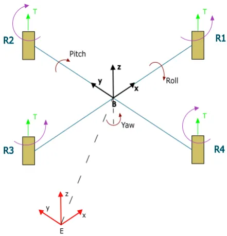
Small unmanned aerial vehicles (SUAV) are used in a great variety of application fields [1–3]. In order to achieve the required level of performance, the vehicle must include a proper automatic control system as well as electronics, sensors, communications, and signal processing algorithms. To develop and validate the control system is very useful to count with an accurate mathematical model of the vehicle, sensors and actuators dynamics [4–12,14]. The present work uses the model structure exposed in [6,12,15] as a starting point but, as a novel contribution, introduces a nonlinear time-varying mathematic model of the rotors used in the DJI F-450 quadrotor (Figure1), that is used to perform a more detailed and realistic analysis of the control system through numerical simulations.

One crucial concern to allow the indoor operation of a SUAV is the attitude and position estimation, typically based on the use of inertial measurement units (IMU) and cameras [6,8,17–21]. To estimate the attitude, position and velocity state variables of the vehicle from the measurements provided by the sensors, a variety of methods are used, such as Kalman filters (KF) [6,18,22,23], extended Kalman filters (EKF) [23-25] and complementary filters [4,27] among others.

Figure 1.Real system modeled in the present work,[16].

Several methods have been published to control the fly of SUAV [1,2,5,9–11,13,14,28–35]. In the present work, we propose a control law structure based on a combination of PID and LQR/LQG algorithms but, in contrast to those exposed in others works [5,30–35], a modified LQR/LQG controller is used to obtain the optimal pre-tuning parameters of four PID controllers, commonly employed for attitude and altitude control in multirotor systems (hover maneuver). Additionally, the uncertainty affecting the measurements are taken into account through the errors and noise modeling of a LIDAR, an optical flow camera, and a MEMS type MARG (Magnetic, Angular Rate, Gravity) sensor. The attitude of the vehicle is estimated using the sensor fusion algorithm proposed in [36], whereas the altitude and the vertical velocity are estimated by means of a Kalman filter. Thus, this study considers the effects of measurement errors, including the relatively large bias and noise errors inherent to the MEMS sensors technology, and includes all the required estimation and compensation algorithms necessary for implementation in a real system. A horizontal controller is also included to analyze the influence of an external control loop over the proposed modified LQR/LQG. Next, we study the performance and the robustness of the proposed pre-tuning method through numeric simulations, considering the non-linear model, particularized for the DJI F-450 quadrotor, as well as the rotors dynamics. The influence of uncertainty and bounded perturbations on the robustness of the method is also tested adding parametric uncertainty and significant external disturbances.

The organization of this paper is as follows: In Section 2, the mathematical model obtained experimentally, which is used to the analysis and evaluation of the control system, is presented, followed by a simplified model used in the design thereof. In Section 3, the proposed design methodology to obtain the attitude and altitude control laws, as well as the employed state estimation algorithms, are described. In Section 4 address the problem of the estimation and control of the horizontal position. Section 5 provides numeric simulation results. Finally, conclusions are drawn in Section 6.

2. Mathematical model

To carry out the synthesis and evaluation of the control system two different models of the DJI F-450 quadrotor will be developed. In the first place, a non-linear model to analyze and evaluate (AEM model) the designed controllers. This model incorporates the effects of the rotors dynamics and the measurement errors. In the second place, a non-linear model for control system design (CDM model). This model includes some simplifications compared with the previous one that will lead to a linear model. The linear model is used to design the controllers and in several estimation algorithms.

2.1. Analysis and evaluation model (AEM)

mu˙ = (cosφsinθcosψ+sinφsinψ)Tb−Kdxu|u| mv˙= (cosφsinθsinψ−sinφcosψ)Tb−Kdyv|v| mw˙ = (cosφcosθ)T_b−K_dzw|w| −mg

Tb =T1+T2+T3+T4

(1)

where(xE,yE,zE)is the position vector of the vehicle relative to the Earth frame,(u,v,w)is the linear velocity (u=x˙E,v=y˙E,w=z˙E), andTbis the total thrust force generated by the four rotors relative to the Body reference frame. On the other hand, the rotational dynamics is described by:

Ixxp˙ = (T2−T4)l−qr(Izz−Iyy) Iyyq˙= (−T1+T3)l−pr(Ixx−Izz)

Izzr˙=

−N12+N22−N32+N42

KP−(Iyy−Ixx)qp ˙

φ= p+q sin(φ)tan(θ) +r cos(φ)tan(θ)

˙

θ=q cos(φ)−r sin(φ)

˙

ψ=q sin(φ)sec(θ) +r cos(φ)sec(θ)

(2)

where (φ,θ,ψ) represents the attitude using Euler angles, (p,q,r) is the angular velocity vector

(measured in the Body frame), Ti is the thrust force generated by thei rotor (relative to the Body frame), andNiis the rotation frequency of theirotor (in RPM), fori∈ {1, 2, 3, 4}.

Figure 2.Earth (E) and Body (B) reference frames.

Table 1.Model parameters of the DJI F-450 quadrotor used for analysis and evaluation.

Simbol Description Value

Kdx Aerodynamic drag coeficient using a reference

area perpendicular toxaxis

0.01212 Kg/m Kdy Aerodynamic drag coeficient using a reference

area perpendicular toyaxis

0.01212 Kg/m Kdz Aerodynamic drag coeficient using a reference

area perpendicular tozaxis

0.0648 Kg/m KT1 Thrust—RPM quadratic relation 1.0155×10−7N/RPM2 KT2 Thrust—RPM gain −1.0327×10−4N/RPM

KP Torque—RPM quadratic relation 3.46×10−8N m/RPM2

Kf Thrust—Duty cycle gain 0.0667 N/%

l Distance from the center of one motor to the center of gravity of the system

0.235 m

m System mass 1.250 Kg

Ixx Moment of inertia aboutxaxis 0.0094 Kg m2

Iyy Moment of inertia aboutyaxis 0.01 Kg m2

Izz Moment of inertia aboutzaxis 0.0187 Kg m2

g Gravitational acceleration 9.81 m/s2

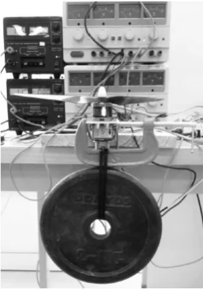
The inputs of the subsystem composed by the electronic speed controllers (ESC), the brushless motors, and the propellers are the duty-cycles values of the PWM signal applied to each ESC,Di, and its outputs are the thrust forces and torques developed by each rotor. Despite the model structure is based on that has been proposed by [6], [12], [15], its parameters have been identified to obtain a trustworthy model of these parts of the DJI F-450 quadrotor. The identification has been carried out applying step and ramp signals to the inputs (Di) and recording the rotation frequencies, thrusts, and torques. The following equipment has been used to accomplish the tests: a calibrated SEN-CC-FZ1439 load cell, a QDR1114 optical sensor functioning as a tachometer, an NI USB-6211 acquisition system, and an LPC4088-32 microcontroller development board. Figure 3 shows one of the experimental set-ups. The reference [37] provides further details.

Figure 3.Experimental setup to characterize the motor thrust.

Each group ESC-motor-propeller is modeled as a first-order system with delay, whose dynamics is described by

whereτis the system time constant,τdis the delay, andKis the stationary gain. The values derived experimentally in the hover equilibrium condition were:τ=0.038s,τd=0.012syK=82.3RPM/%. The experimental relations that link the rotational frequencyN(in RPM) with the thrust,T, and the torque,P, developed by each rotor are given by the Equations (4) and (5), respectively.

T=KT1N2+KT2N (4)

P=KPN2 (5)

In order to carry out a realistic analysis and design, the errors and noise levels of conventional commercial sensors employed in these type of systems have been obtained from the manufacturer manuals and introduced in the model. These sensors are a PulsedLight LIDAR-LITE laser range sensor [38], an InvenSense MPU-9250 MARG [39], [40], comprising a 3-Axis gyroscope, a 3-Axis accelerometer, and a 3-Axis magnetometer [38, 39], and a PX4-FLOW optical flow camera [41].

2.2. Control system design model (CDM)

To ease the task of designing the controller, we will build a simplified model relative to the one presented in the previous section. The main differences between the two are the followings:

• The CDM model does not take into account the rotor dynamics.

• The thrust and the torque are linear functions of the PWM signals duty-cycle.

• The rotational dynamical model assumes relative low angular velocities and small enough Euler angles.

After applying the cited simplifications, the CDM model is defined by the system of non-linear Equations (6). Table1shows the parameter values of this model.

p=φ˙, q=θ˙, r=ψ˙

Ixxp˙ =Uφ−qr(Izz−Iyy)

Iyyq˙=Uθ−pr(Ixx−Izz)

Izzr˙=Uψ−qp(Iyy−Ixx)

u=x˙E, v=y˙E, w=z˙E

mu˙ = (cosφsinθcosψ+sinφsinψ)Uz−Kdxu|u| mv˙= (cosφsinθsinψ−sinφcosψ)Uz−Kdyv|v| mw˙ = (cosφcosθ)Uz−Kdzw|w| −mg

(6)

The relations between the components of theUandDvectors (the duty-cycles of the four PWM signals) is defined by [6]:

    

Uφ

Uθ

Uψ

Uz      | {z }

U

=

    

0 Kfl 0 −Kfl

−Kfl 0 Kfl 0

−KP KP −KP KP

Kf Kf Kf Kf     

| {z }

M

    

D1 D2 D3 D4

     | {z }

D

(7)

whereDis the vector of duty-cycles, and the components ofUare the fictitious control signalsUφ,Uθ,

choose between considering the whole 4x4 MIMO problem or one 3x3 MIMO attitude problem plus one SISO altitude problem instead. The next section elaborates on the first option.

3. Attitude and altitude control system

The main objective of this system is the stabilization (hovering) of the vehicle at a certain altitude. Hovering is a maneuver in which the quadrotor is maintained in nearly motionless flight over a reference point at a constant altitude and on a constant heading. In order to control the vehicle, the complexity of the system and the strong coupling that exists between the manipulated variables and the controlled variables has been taken into account. Therefore, a multivariable control approach based on state space has been considered [42–44]. As a novel contribution of this work for multivariable PID tuning, it is proposed to use a modified LQR/LQG control law, in which feedback is performed considering the tracking error between the state vector and a setpoint or reference state vector. In concrete, for the design of the attitude and altitude controller the following state vector,X, is considered:

XT=φ θ ψ zE p q r w

(8)

The manipulated variables (MV) vector,U, is composed of the four componentsUφ,Uθ,UψandUz

given in (6). The process variables (PV) vector, or controlled variables (CV) vector, is given by,

YT =φ θ ψ zE

(9)

An equilibrium condition for hovering at an altitudezeqis characterized by,

XTeq =

0 0 0 zeq 0 0 0 0

, UTeq=

0 0 0 Uzeq

, YTeq =

0 0 0 zeq

(10)

Linearizing the eight non-linear differential equations of the quadrotor model (6) for hover condition, (Xeq, Ueq, Yeq), and considering incremental (or deviation) variables with respect to equilibrium point,

x=X−Xeq, u=U−Ueq, y=Y−Yeq (11)

the linearized system dynamics is defined by (12).

˙

x=Ax+Bu

y=Cx (12)

In order to add integral action to the controller, the system model is modified including four new state variables corresponding to the integral of the tracking error of the controlled variables, resulting the following augmented state vector,

xA = x

xI !

(13)

where ˙xI =r−y, andris the incremental value of the set-point vector,r=YSP−YSPeq. Therefore, the augmented system matrices are given by,

Aa= A 0

−C 0

!

, Ba= B 0

!

, Ca=

C 0 (14)

The conventional LQR control law with integral action (incremental vector value) is given by,

and the controller output (CO) vector (U) is obtained by,

U=Ueq+u (16)

For that, the feedback gain matrices,KcandKI, must be calculated solving the corresponding algebraic Riccati equation (AREc) [42–44], which results from the optimization problem of minimizing a cost function given by,

J=

Z ∞ 0

xTQcx+uTRcudt (17)

whereQcandRcare the named weighting matrices.

With the LQR controller, the linearized closed loop control system dynamics (which is an approximation of the nonlinear system for a neighborhood of the equilibrium point defined by the hover condition) is given by,

˙ x ˙ xI

!

= (Aa−BaKca)

| {z } Ayr

x xI

!

+Byrr, Kca= (Kc −KI) (18)

A proposal made in this work is to modify the conventional LQR structure given in (15), where the new control law is defined by,

u=Kc(xSP−x) +KIxI (19)

wherexSPrepresents the incremental reference (or set-point) state vector to follow,

xT_SP=φSP θSP ψSP zSP pSP qSP rSP wSP

(20)

The proposed control law (19) gets the same poles for the closed loop linearized system obtained with (15), but achieves to reduce the time response of the system to set-point changes due to (19) modifies the zeros of the closed loop system reached with (15).

3.1. Pre-tuning method for attitude and altitude controller

The aim of a pre-tuning procedure is to determineQcandRcweighting matrices in (17) for which a suitable solution is obtained. For that, diagonal weighting matrices have been chosen,

Qc=diag(qφ,qθ,qψ,qz,qp,qq,qq,qr,qIφ,qIθ,qIψ,qIz) (21)

Rc=diag(ρφ,ρθ,ρψ,ρz) (22) Taking into account experimental (computer simulations) observations behaviour of the closed loop system, and physical meaning of the relative values used in the elements of the weighting matrices, the following relations are proposed as starting point:

qθ =qφ, qψ=qφ/7, qz =qφ/35 (23)

qp=qφ/70, qq =qp, qr =qp/5, qw=qp (24)

qIφ=qp/2, qIθ=qIφ, qIψ=qIφ/5, qIz=qIφ (25)

ρφ=qφ/4, ρθ=ρφ, ρψ =ρφ/3, ρz=ρφ/30 (26)

in this way, for a givenqφparameter value, the rest of weighting parameters are calculated for the

In order to analyze the properties of the proposed controller, an illustrative example is shown below, where the following tuning parameters have been adjusted experimentally,

Qc=diag(350, 350, 50, 10, 4, 5, 1, 4, 3, 3, 1, 4) (27)

Rc=diag(88, 88, 32, 3) (28)

With these weighting matrices, the following state feedback matrices,KcandKi, are obtained,

Kc=     

2.9394 0.0000 −0.0000 0.0000 0.3174 0.0000 0.0000 0.0000 0.0000 2.9408 0.0000 0.0000 0.0000 0.3401 0.0000 0.0000 0.0000 0.0000 0.5024 0.0000 0.0000 0.0000 0.1542 0.0000 0.0000 0.0000 0.0000 2.7333 0.0000 0.0000 0.0000 2.8867

     (29)

KI =     

0.1846 0.0000 −0.0000 0.0000 0.0000 0.1846 0.0000 0.0000 0.0000 0.0000 0.0079 −0.0000 0.0000 −0.0000 −0.0000 1.2247

     (30)

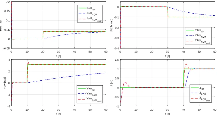
In order to analyze the effect of the modified LQR control law, in Figure4it is shown a comparative between the time response of the linearized system employing the conventional control law (15) and the proposed control law (19). In both cases the initial state vector isxT_i (0) = (0.1,−0.3,π,−1, 0, 0, 0, 0),

expressed in the international units system. As it can be seen, the control law (19) achieves a significantly faster time response.

0 10 20 30 40 50 60

t [s] -0.05 0 0.05 0.1 0.15 0.2 Roll [rad] Roll_SP Roll_LQR Roll_LQR modf

0 10 20 30 40 50 60

t [s] -0.4 -0.3 -0.2 -0.1 0

Pitch [rad] PitchSP

PitchLQR

PitchLQR

modf

0 10 20 30 40 50 60

t [s] -4 -2 0 2 4

Yaw [rad] YawSP

YawLQR

YawLQR

modf

0 10 20 30 40 50 60

t [s] -1 -0.5 0 0.5 1 1.5 Z [m] ZSP ZLQR ZLQR modf

Figure 4.Comparative of closed-loop systems obtained with control laws (15) and (19).

The proposed controller can be interpreted as a multivariable PID controller for a MIMO (4x4) system, taking into account that theKcmatrix can be expressed as

Kc= [KP KD]

KP=     

2.9394 0.0000 −0.0000 0.0000 0.0000 2.9408 0.0000 0.0000 0.0000 0.0000 0.5024 0.0000 0.0000 0.0000 0.0000 2.7333

    

, KD=

    

0.3174 0.0000 0.0000 0.0000 0.0000 0.3401 0.0000 0.0000 0.0000 0.0000 0.1542 0.0000 0.0000 0.0000 0.0000 2.8867

where the respectiveKP,KD(29) andKI(30) matrices are practically diagonal matrices, and therefore they can be approximated by

KP =     

KPφ 0 0 0

0 KPθ 0 0

0 0 KPψ 0

0 0 0 KPz

    

, KI =     

KIφ 0 0 0

0 KIθ 0 0

0 0 KIψ 0

0 0 0 KIz

    

, KD=     

KDφ 0 0 0

0 KDθ 0 0

0 0 KDψ 0

0 0 0 KDz

    

(32) With these approximations, the PID control laws (using Laplace transform domain) for the components of the controller out vector are given by,

uφ(s) =KPφeφ(s) +

KIφ

s eφ(s) +sKDφeφ(s)

u_θ(s) =KPθeθ(s) +

KIθ

s eθ(s) +sKDθeθ(s)

uψ(s) =KPψeψ(s) +

KIψ

s eψ(s) +sKDψeψ(s)

uz(s) =KPzez(s) + KIz

s ez(s) +sKDzez(s)

(33)

whereeφ,eθ,eψandezare the respective tracking error signals for the controlled variables,φ,θ,ψand

zE. Figure5shows block diagrams with the conventional LQR and the modified LQR control laws.

LQR

Kc

1

s Ki

SP

Y Y

Y E _U

SP

X

(a)

Modified LQR

Y Ki

1 s

Kp

Kd SP

SP

Selector

X

Y Y

U E

SP

SP

(p, q, r, w)

(b)

Figure 5.(a) Control Law LQR (15). (b)Control Law modified LQR (19).

Once the controller output vectorUhas been calculated, the duty cycle vector,Dfor the PWM signals applied to motors are obtained taking into account Equation (7),

In order to implement the proposed algorithm, all state variables are needed for feedback. For that, and taking into account the characteristics of the system to control, low-cost commercial sensors characteristics are used in computer simulations based on data sheets given by manufacturers. A MARG (Magnetic, Angular Rate, and Gravity) sensors system (MPU-9250 model, with 3-axes accelerometer, rate-gyro and magnetometer) is used for attitude and orientation measurements ([39], [40]). A LIDAR (Light Detection and Ranging) is used for altitude measurement ([38]). Due to bias/drif effects acting on measurements given by inertial sensors, compensation algorithms must be considered as it is described in next Section.

3.2. Attitude estimation

In order to achieve proper control of the system is very important to have attitude measurements accurate enough. The references [45] and [46] compares the performance of three sensor fusion algorithms that use the MARG measurements for attitude estimation. These are an extended Kalman filter (EFK), the non-linear complementary filter (NLCF) described in [27]], and the error optimization algorithm detailed in [36] based on the gradient descent method (MHV). Table2shows the relative computation times on a typical embedded system as well as the RMS errors for the three algorithms. This work uses the MHV algorithm since it has a good compromise between computation cost and estimation errors.

In each sample interval, the MHV algorithm proceeds first finding the best alignment between the gravity and Earth magnetic vectors and those measured by the accelerometer and the magnetometer, respectively. To get that optimal alignment of these two pairs of vectors despite the presence of measurement errors the MHV algorithm uses the gradient descent method. The output of this stage is a quaternion (B_Eq˙w,t) presenting the rate of change of the attitude. This quaternion is then combined with the obtained from the angular velocity measured by the gyroscope (B_Eq˙w,t) to calculate a better estimation (Figure6) using

B

Eq˙est,t=BEq˙w,t−βB_Eq˙ˆe,t, (35) whereβis an adjustable weighting factor representing the gyroscope measurement error expressed

as the magnitude of a quaternion derivative. The algorithm also copes with the effects of magnetic disturbances and the bias present in the gyroscope.

, est t B E

q



[rad/s]

Accelerometer measurements normalized vector

Magnetometer measurements normalized vector

Rate of change of orientation quaternion

β

ʃ

1

||𝑞𝑞||

,

ˆ

q



+

-,

B E

q



Optimal

alignment

with

gravity

and magnetic

vectors

in Earth

frame

The angular velocity vector (p,q,r) is supposed to be taken directly from the gyroscope output and, for simulation purposes, is degraded with the noise levels stated in the datasheet [39].

Table 2.RMSE in dynamic conditions and compute time of the three attitude estimation algorithms considered, [46].

Parameter EKF MHV NLCF

RMSE Roll [◦] 4.71 4.85 5.07 RMSE Pitch [◦] 1.91 2.65 2.89 RMSE Yaw [◦] 5.19 5.13 5.67 Compute time [ms] 2.7 0.15 0.11

3.3. Estimation of linear velocity and position in axis zE

The sensor LIDAR-LITE [38] gives a measurement from the quadrotor to ground, which can be used for estimating the vertical velocity and position. For that, taking into accoint the model given in (6), only the equations corresponding to ˙zEand ˙ware considered, and it is supposed thatφandθ

takes values next to zero (which is a good approximation for hover maneuver); with what turns out Equation (36).

˙

w= 1

m(Uz−Kdzw|w|)−g

˙

zE =w

(36)

If (36) is linearized for hover condition (weq=0,zeq=0,Uzeq), a linear Kalman filter (KBF) can

be used forw,zEestimation. Covariance matrices, (Qo,Ro) must be adjusted to obtain a satisfactory KBF. For that, an experimental iterative procedure has been applied, obtaining the following matrices, whereRotakes into account the noise measurement gives by [38],

Qo = 200 0

0 0.001

!

, Ro=0.05 (37)

The stationary observer gain matrix,Ko, can be obtained solving the corresponding observer algebraic Riccati equation (AREo) [42–44]. In this way, results an LQG controller, and the complete attitude-altitude controller is a combination of LQR (for attitude control) and LQG controller (for altitude control), named in this work as LQR/LQG. A block diagram with the complete structure of the control system is shown in Figure7.

4. Horizontal position controller

Equation (38) shows the control laws generated by the PIDs with filter to derivative action, employing the Laplace transform notation. Controllers parameters have been obtained experimentally, and are given in Table3(the negative sign is due to the sign criterium used forφandyB, see Figure2).

SPφ(s) =KPeyB(s) + KI

s eyB(s) + KDs

τ_{f D}s+1eyB(s)

SPθ(s) =KPexB(s) + KI

s exB(s) + KDs

τf Ds+1exB

(s)

(38)

whereexB andeyB are the error components of the horizontal position vector (eH) which are referenced

to the boty-axis reference system.

(φSP, ΘSP)

M

U D

Limit and Balance Duty Cicles

D1 D2 D3 D4 LIDAR

Efficient Orientation Fusion Filter

(MHV)

Stationary Kalman Filter Rotation

Uz

(p, q, r)

MARG

Gyroscope (3 axes) Accelerometer (3 axes) Magnetometer (3 axes)

(z, w)

(xSP, ySP) z

PX4FLOW Scaled Rotation

(x, y) _(e x, ey)

Rotation _PID

(ΨSP)

Filters

Filter

Limits

LQRM

LQG

LQRM

(zSP)

Filter zSP

xSP, ySP (φ, Θ)

(φ, Θ, Ψ)

-₊

Ψ

ΨSP

(Uφ,UΘ,UΨ)

Figure 7.Complete control system diagram for attitude, altitude and horizontal position. Blocks with LQRMreferences the modified LQR (19).

Table 3.Coefficients of the position controller.

KP KI KD τf D[s]

SPφ -0.050 -0.0025 -0.08 1

SPθ 0.050 0.0025 0.08 1

The horizontal positioning error can be referenced with respect to body-axes reference system, eH(exB,eyB), as well as to the Earth-axes reference system,eH(exE,eyE). For small values ofφandθ

angles, the relation between the horizontal coordinates is given by,

exB eyB

!

= cos(ψ) sin(ψ)

−sin(ψ) cos(ψ)

! exE eyE

!

4.1. Horizontal position estimation

The horizontal position estimation of the quadrotor derives from a CMOS optical flow camera model PX4FLOW [41] pointing down. This camera computes a displacement vector utilizing the correlation between successive images, so its output is expressed in pixels units and not in real units. To compute the truth velocity is necessary to take account the focal length of the camera lens as well as the distance from the camera to the floor, or altitude, that is already available from the LIDAR, as is shown in Equation (40). Also, the horizontal velocity has to be rotated (41) taking into account theψ

angle estimated previously to refer it to the Earth frame. Then, the horizontal velocity is integrated to get the final horizontal position in that frame (xE,yE).

vxB vyB

!

= vx

vy !

z

f (40)

wherezis the distance to the floor and f is the focal distance of the camera lens. The manufacturer states that the average error in the camera output is zero, so the position measurement drift should be negligible.

vxE vyE

!

= cos(ψ) −sin(ψ)

sin(ψ) cos(ψ)

! vxB vyB

!

(41)

5. Results

This section presents the results obtained, in a realistic simulation scenario, when analyzing the LQR/LQG controller modified for the attitude and the altitude proposed in this paper. For this purpose, an analysis of the performance of this control system is carried out by applying it to the AEM model of the quadrotor. The non-linear model AEM, (1) and (2), also takes into account: rotor dynamics (3), measurement errors [38–41], the effect of estimation algorithms (MHV and KBF) and the effect of adding an external control loop for the horizontal position (38) of the quadrotor. This framework is illustrated in Figure7, which shows the interaction between measurements provided by sensors, estimation algorithms and controllers. It should be mentioned that in all the simulations presented the numerical integration method of Runge-Kutta of fourth order with an integration step of 0.1 ms has been used. The estimation (MHV and Kalman filter) and control algorithms are executed at a frequency of 400 Hz in simple arithmetic precision. The discretization of the controllers and the Kalman filter is carried out using the Euler backward method, and β = 0.01 is used in the MHV

algorithm for fusion of sensor data. To conclude, a robustness analysis of the attitude and altitude control system to parametric uncertainty and to different types of external disturbances has been realized.

Before the attitude and altitude control performances are analysed, the MARG MPU-9250 sensor modelling is shown in Figure8. As can be seen, all measurements are affected by noise and bias levels according to the values indicated by the manufacturer [39]. In addition, in the case of accelerometers, the measurement provided (axm) is affected by both gravity (axg) and the linear accelerations experienced by the quadrotor (axl). This consideration has a negative effect on the estimation of the attitude made by the MHV algorithm, which can be seen in Figure9. As a comparison, this figure also shows the result of integrating the angular velocities provided by the MARG directly to estimate the attitude. This integration diverges with time due to the bias effect present in the measured angular velocities (pm,qm,rm). On the other hand, the Kalman Filter for altitude and linear velocityw gets to estimate these state variables accurately, see Figure10. This is in part due to the quality of the measurements provided by the sensor Lidar-Lite [38]. Once the estimated/measured state vector is presented, it can be pointed out that the most negative effect is present in the attitude estimation; the attitude controller must be robust to the coupling presented between the estimate of the angles (φ,θ)

5 10 15 t (s) -0.5 0 0.5 1 ax b (m/s 2) ax m ax g ax l

5 10 15

t (s) -1.5 -1 -0.5 0 0.5 ay b (m/s 2) ay m ay g ay l

5 10 15

t (s) -15 -10 -5 0 5 az b (m/s 2) az m az g az l

5 10 15

t (s) -0.4 -0.2 0 0.2 0.4 p (rad/s) p m p

5 10 15

t (s) -0.4 -0.2 0 0.2 0.4 q (rad/s) q m q

5 10 15

t (s) -0.3 -0.2 -0.1 0 0.1 r (rad/s) r m r

5 10 15

t (s) 24 26 28 30 32 mx b ( T) mx m mx

5 10 15

t (s) -20 -15 -10 -5 0 my b ( T) my m my

5 10 15

t (s) -32 -31 -30 -29 -28 mz b ( T) mz m mz

Figure 8.Modelling of the measurements provided by the MARG MPU-9250 on body axes (B) when it

is fixed to the quadrotor system.

0 10 20 30 40 50

t (s) -5 0 5 10 15 20 Roll (degree) Roll Roll_est

pmdt

0 10 20 30 40 50

t (s) -8 -6 -4 -2 0 2 4 6 Pitch (degree) Pitch Pitch_est

qmdt

0 10 20 30 40 50

t (s) -5 0 5 10 15 20 25 30 Yaw (degree) Yaw Yaw_est

rmdt

Figure 9.Attitude of the quadrotor system versus the attitude estimated by the MHV algorithm and the attitude obtained by integrating the measured angular velocities directly.

0 5 10 15 20 25 30 35 40 45 50

t (s) -1 0 1 2 3 4 z (m) z m z z_est

0 10 20 30 40 50

t (s) -1.5 -1 -0.5 0 0.5 w (m/s) w w_est

With the state vector used for the attitude and altitude controller feedback presented, the results obtained when applying this controller to the AEM mathematical model are shown. In Figure11can be seen how the modified LQR/LQG control gets that the system follows the setpoints requested for (φ,θ,ψ,z) adequately, despite: measurement errors (Figure8), estimation errors (Figures9and10)

and uncertainty in the AEM model with respect to the linear design model. It should be noted that for both attitude and altitude, the error between the estimated variable and the requested setpoint is quite small (±0.2 degrees forφestandθest). Therefore, if sensoric and/or estimation algorithms of superior performance are available, the following of setpoints carried out by this controller would have a considerable improvement margin. The duty cycles (D) generated by the modified LQR/LQG controller to get the above tracking are shown in Figure12.

0 5 10 15 20 25 30 35 40 45 50

t (s)

-1 0 1 2 3 4 5 6

Roll (degree)

Roll_sp

Roll Roll est

0 10 20 30 40 50

t (s)

-1 0 1 2 3 4 5 6

Pitch (degree)

Pitch_sp

Pitch

Pitch_est

0 5 10 15 20 25 30 35 40 45 50

t (s)

-5 0 5 10 15 20 25 30

Yaw (degree) _Yaw

sp Yaw Yaw est

0 10 20 30 40 50

t (s)

-1 0 1 2 3 4

z (m)

z_sp

z z est

Figure 11.φ,θ,ψandzof the closed-loop system, estimates and setpoints.

0 5 10 15 20 25 30 35 40 45 50

t (s)

50 55 60 65 70 75 80

D (%)

Rotor1

0 10 20 30 40 50

t (s)

50 55 60 65 70 75 80

D (%)

Rotor2

0 5 10 15 20 25 30 35 40 45 50

t (s)

50 55 60 65 70 75 80

D (%)

Rotor₃

0 10 20 30 40 50

t (s)

50 55 60 65 70 75 80

D (%)

Rotor₄

On the other hand, most high-level applications of SUAV systems require the vehicle to be able to track position commands in space or maintain static positions. Therefore, it is necessary to validate the attitude and altitude controller proposed in this paper by adding an external control loop (38) for the horizontal position of the system. As shown in Figure13, the closed-loop system resultant gets a satisfactory tracking of the setpoints demanded for the positions (xE,yE,zE). Since the modified LQR/LQG control achieves, even with the estimation errors committed by the MHV algorithm (due to the linear accelerations experienced by the system), to follow rapidly the setpoints (φspandθsp) demanded by the horizontal position controller. Furthermore, the proposed control structure is valid for tracking complex trajectories. Figure14shows the position in the quadrotor space when tracking ascending circular paths. It can be seen that despite the coupling of the system and the errors present in the estimates and measurements, the results obtained can be considered satisfactory in terms of stabilization and setpoint tracking, although they can be improved by controllers fine tuning.

10 20 30 40 50 60 70

t (s) -6 -4 -2 0 2 4

Roll (degree) Roll_sp

Roll Roll_est

10 20 30 40 50 60 70

t (s) -2 -1 0 1 2 3 4 Pitch (degree) Pitch_sp Pitch Pitch_est

10 20 30 40 50 60 70

t (s) -40 -20 0 20 40 60 80 Yaw (degree) Yaw_sp Yaw Yaw_est

10 20 30 40 50 60 70

t (s) -0.5 0 0.5 1 1.5 2 x (m) x_sp x x est

10 20 30 40 50 60 70

t (s) -1.5 -1 -0.5 0 0.5 1 1.5 y (m) y_sp y y_est

10 20 30 40 50 60 70

t (s) 0 1 2 3 4 5 z (m) z_sp z z_est

Figure 13.AEM model when applying the control and estimation structure shown in Figure7.

0 -0.5 0.8 0.5 1 0.6 1.5 zE ( m ) 2 0.4 2.5 3 0.2 0.2 3.5 0 yE (m)

-0.2 0

-0.4 -0.2

xE (m) -0.6 -0.8 -0.4 -1 -1.2 -0.6 -1.4 -0.8 -1.6 Path_est Path Pathsp

5.1. Robustness Analysis

In order to study the robustness of the modified LQR/LQG structure proposed in this work, for the pre-tuning of PID controllers applied to quadrotor systems, an analysis of attitude and altitude control is performed by adding: parametric uncertainty to the system inertia (which will determine the system response speed) and parametric uncertainty to the gain of the SISO model identified for the rotors. On the other hand, the robustness of the modified LQR/LQG control by exposing the quadrotor system to significant external disturbances (torques and forces) is also studied. Furthermore, in both cases all measurement/estimation errors presented in the previous section are considered.

5.1.1. Parametric Uncertainty Robustness Analysis

In this analysis, the inertia moments of the AEM model, collected in Table1, have been multiplied by a gain of∆I. Specifically, the inertia moments of the system have been varied in an interval [−17.5, 17.5]%. The study focuses on this parameter becauseIxandIyare the ones that determine the fastest dynamics of the quadrotor and, therefore, those that affect in greater measure to the system when determining the performance of the attitude control. The study of the added uncertainty in the mass of the system has not been carried out, since this can be known with sufficient precision and does not vary with time. As result of the study, Table4shows the values obtained when calculating the IAE (Integrated Absolute Error) of all controlled variables (x,y, z,φ, θ, ψ) in function of the

uncertainty added to the inertia moments. In addition, it records the IAu (Integrated Absolute) of the incremental variableu, which is defined as the sum of the incremental duty cycles (d) with respect to the equilibrium condition (Deq). All the simulations carried out to obtain the values listed in Table

4are reproductions of the one shown in Figure13. As can be seen in this table, the low variation of the indicators shows that the modified LQR/LQG controller, together with the horizontal position controller, presents robust behavior to the uncertainty added to this parameter. It should be noted that the magnitude of the IAE indicators decreases considerably if these are calculated with respect to the estimated variables, see Table5. This supports the previously mentioned, the results obtained when applying the control structure proposed in this work to the AEM model have a considerable margin of improvement if the quality of the measures/estimates is increased. As a visual support to the above, Figure15shows the variation of the IAE attitude indicators and the IAu control effort indicator.

Table 4.Performance indicators of controlled variables (I AE) and control effort (I Au) in function of parametric uncertainty added to inertia moments (Iadd).

Iadd[%] I AEX I AEY I AEZ I AEφ I AEθ I AEψ I Au

Table 5. Performance indicators of the estimated controlled variables (I AE) in function of the parametric uncertainty added to inertia moments (Iadd).

I_add[%] I AEXest I AEYest I AEZest I AEφest I AEθest I AEψest

17.5 1.0849 1.0738 5.9441 4.0947 4.4447 9.2150 15.0 1.0871 1.0741 5.9441 4.0536 4.3870 9.0385 12.5 1.0895 1.0746 5.9440 4.0185 4.3410 8.8624 10.0 1.0919 1.0751 5.9440 3.9911 4.3064 8.6862 7.5 1.0941 1.0754 5.9440 3.9774 4.2820 8.5101 5.0 1.0962 1.0759 5.9440 3.9762 4.2724 8.3350 2.5 1.0982 1.0765 5.9439 3.9865 4.2806 8.1609 0 1.0995 1.0771 5.9440 4.0120 4.3068 7.9877 -2.5 1.1007 1.0777 5.9440 4.0513 4.3638 7.8161 -5.0 1.1026 1.0786 5.9440 4.1067 4.4628 7.6468 -7.5 1.1055 1.0806 5.9440 4.1940 4.6223 7.4801 -10.0 1.1090 1.0824 5.9440 4.3763 4.8359 7.3095 -12.5 1.1134 1.0851 5.9442 4.7788 5.1354 7.1386 -15.0 1.1184 1.0927 5.9441 5.5396 5.7354 6.9640 -17.5 1.1398 1.1083 5.9445 7.5210 6.8205 6.8099

-20 -15 -10 -5 0 5 10 15 20

I_add (%)

0 5 10 15 20 25

IAE

act

IAE

IAE

e

IAE

IAE

e

IAE

IAE

e

-20 -15 -10 -5 0 5 10 15 20

I_add (%)

225 230 235 240 245 250 255 260 265 270 275

IA

u

IAu

Figure 15. Variation of the performance indices of the controlled attitude IEA(real attitude vs. estimated attitude) and variation of the control effortI Au, all of them in function of the parametric uncertainty added to the moments of inertiaIadd.

To conclude, Figure16shows the results obtained by adding a parametric uncertainty to: the inertia moments (Iadd = −10%) and the gains of the SISO models identified for the rotors,∆KR =

10 20 30 40 50 60 70 t (s) -4 -3 -2 -1 0 1 2 3 Roll (degree) Roll sp Roll Roll_est

10 20 30 40 50 60 70

t (s) -10 -5 0 5 10 Pitch (degree) Pitch sp Pitch Pitch_est

10 20 30 40 50 60 70

t (s) -40 -20 0 20 40 60 80 Yaw (degree) Yaw sp Yaw Yaw_est

10 20 30 40 50 60 70

t (s) -0.5 0 0.5 1 1.5 2 x (m) x_sp x x_est

10 20 30 40 50 60 70

t (s) -1.5 -1 -0.5 0 0.5 1 1.5 y (m) y_sp y y_est

10 20 30 40 50 60 70

t (s) 0 1 2 3 4 5 z (m) z_sp z z_est

Figure 16.AEM model withIadd=−10% and∆KR= (4,−6, 3.2,−2.9)T% when applying the control

and estimation structure shown in Figure7.

5.1.2. External Disturbance Robustness Analysis

In this section the robustness to significant external disturbances of the modified LQR/LQG control proposed in this paper is studied. First, a scenario in which the AEM model is subjected to external torques that increase until a constant value is established, adding to these torques a stochastic component (simulating a continuous wind). Furthermore, in the same scenario, a significant increase in weight is applied to the quadrotor (one third of its weight) in order to simulate a manoeuvre in which the quadrotor system would elevate a load outdoors for then transport it. The results obtained when carrying out the hover manoeuvre in this scenario are presented in Figure17.

0 10 20 30 40 50 60 70 80

t (s) -1 0 1 2 3 4 5 6 Roll (degree) Roll_sp Roll Roll_est

0 10 20 30 40 50 60 70 80

t (s) -4 -3 -2 -1 0 1 Pitch (degree) Pitch_sp Pitch Pitch_est

0 10 20 30 40 50 60 70 80

t (s) -20 0 20 40 60 80

Yaw (degree) Yawsp

Yaw

Yaw_est

0 10 20 30 40 50 60 70 80

t (s) -1 -0.5 0 0.5 1 1.5 2 2.5 z (m) z_sp z z_est

As shown in the figure above, external disturbances are successfully rejected by the attitude and altitude controller, although the rejection time could be improved if fine tuning to the integral action of the controllers is carried out. It should be added that the stochastic component of the disturbances increases the oscillation in the controlled variables. Especially in the anglesφandθ, although in

this scenario this oscillation can be considered admissible, since it is bounded between[−0.5, 0.5] degrees. The duty cycles generated by the modified LQR/LQG control system and the applied external disturbances are shown in Figure18.

0 20 40 60 80

t (s) 0

0.1 0.2 0.3 0.4

x

(Nm)

0 20 40 60 80

t (s) -0.3

-0.25 -0.2 -0.15 -0.1 -0.05 0

y

(Nm)

0 20 40 60 80

t (s) 0

0.1 0.2 0.3 0.4 0.5 0.6

z

(Nm)

0 20 40 60 80

t (s) -5

-4 -3 -2 -1 0

fz

(N)

0 20 40 60 80

t (s) 50

60 70 80 90

D1

(%)

0 20 40 60 80

t (s) 50

55 60 65 70 75 80

D2

(%)

0 20 40 60 80

t (s) 50

60 70 80 90 100

D3

(%)

0 20 40 60 80

t (s) 50

60 70 80 90

D4

(%)

Figure 18. External disturbances that affect to the AEM model and duty cycles generated by the modified LQR/LQG control to reject them.

Finally, another scenario in which the quadrotor system is exposed to occasional external disturbances (of significant magnitude) while performing the hover manoeuvre is considered. This scenario can occur in obstacle avoidance and path planning missions, in which SUAV systems are often used. Specifically, the external torques and forces to which the AEM model is exposed could be the result of punctual collisions with different obstacles, as a result of a fault in the avoidance system. In addition, in order to create an unfavorable scenario, an uncertainty ofIadd=−10% has been added to the inertia moments of the AEM model and an uncertainty∆KR= (−2.5, 2,−2.3,−2.2)% is also added to the gains of the SISO models identified for the rotors. The results obtained in this scenario are presented in Figures19and20. As it can be seen, the magnitude of the external punctual torques makes that the system deviates considerably (25 and−22.5 degrees in the anglesφandθ, respectively)

from the equilibrium position hover, for which the modified LQR/LQG control has been designed. Moreover, the punctual torque on thezBaxis causes an undesired turn of 45 degrees on theψangle.

0 10 20 30 40 50 60 70 80 t (s) -5 0 5 10 15 20 25 30 Roll (degree) Roll_sp Roll Roll_est

0 10 20 30 40 50 60 70 80

t (s) -25 -20 -15 -10 -5 0 5

Pitch (degree) Pitchsp

Pitch

Pitch_est

0 10 20 30 40 50 60 70 80

t (s) -20 0 20 40 60 80 100 Yaw (degree) Yaw_sp Yaw Yaw_est

0 10 20 30 40 50 60 70 80

t (s) -1 -0.5 0 0.5 1 1.5 2 2.5 z (m) z_sp z z_est

Figure 19.Model AEM of the quadrotor with added parametric uncertainty carrying out maneuver hover while it is exposed to the set of external punctual disturbances shown in Figure20.

0 20 40 60 80

t (s) 0 0.2 0.4 0.6 0.8 1 x (Nm)

0 20 40 60 80

t (s) -1.2 -1 -0.8 -0.6 -0.4 -0.2 0 y (Nm)

0 20 40 60 80

t (s) 0 0.2 0.4 0.6 0.8 1 1.2 z (Nm)

0 20 40 60 80

t (s) -2.5 -2 -1.5 -1 -0.5 0 fz (N)

0 20 40 60 80

t (s) 30 40 50 60 70 80 90 D1 (%)

0 20 40 60 80

t (s) 30 40 50 60 70 80 90 100 D2 (%)

0 20 40 60 80

t (s) 50 60 70 80 90 100 D3 (%)

0 20 40 60 80

t (s) 50 60 70 80 90 100 D4 (%)

Figure 20.External punctual disturbances that affect to the AEM model and duty cycles generated by the modified LQR/LQG control to reject them.

5.2. First pre-tuning tests on the real system

(a)

7

6 9

4 3

5 2

8

1

(b)

Figure 21. (a) Real system used in tests. (b) Main parts of the PCB: (1) Connections with external sensors, (2) flight unit PCBs, (3) Barometer, (4) MARG, (5) GPS, (6) Microcontroller, (7) LEDs and buzzer, (8) Rotor connections, (9) Power supply. The radius of the PCB is 6.75 cm.

The Figure22shows the attitude (φ,θ,ψ) of the quadrotor during takeoff. As it can be seen, the

modified LQR controller needs a few seconds to get that the quadrotor follows the attitude setpoints demanded. After this transitory, the system follows the demanded setpoints with a tracking error bounded between±2 degrees. These results are less favorable than those obtained with the simulated model but could be improved by fine tuning the controller. This is due to the fact that there will always be differences between the real system and the simulation. These differences are mainly due to the uncertainty in the model used for design, as well as possible disturbances acting on the system.

0 5 10 15 20

-5 0 5 10

Roll(

degrees

)

Rollest

RollSP

0 5 10 15 20

-2 -1 0 1 2 3 4 5 6

Pitch(

degrees

) PitchPitchestSP

0 5 10 15 20

t (s)

-10 -5 0 5 10 15 20 25 30

Yaw(

degrees

) YawYawestSP

t (s)

t (s)

Figure23shows the behavior of the multirotor for setpoint changes in altitude (zE). An acceptable average tracking error is obtained for a pre-tuning stage, and the maximum transient error is limited to±0.07 m. Finally, [47] presents a video in which the real quadrotor system is affected by significant external disturbances. As can be seen in this video, the pre-tuning method proposed in this work obtains a robust attitude and altitude controller to significant external disturbances.

0 20 40 60 80 100 120 140

0 0.5 1

0 20 40 60 80 100 120 140

0 0.5 1 1.5 2

z

z

0 20 40 60 80 100 120 140

0 0.5 1 1.5 2

Sp_z z z_f

z(

m

)

t (s)

Figure 23.Height of the real quadrotor in closed loop (modified LQG controller). 6. Conclusions

A method for pre-tuning a multivariable PID controller for a quadrotor attitude and altitude control has been proposed, which is based on LQR/LQG theory, using a modified structure of the LQR, where the state feedback algorithm employs the tracking error vector instead of the state vector. Realistic computer simulations have been carried out using a nonlinear mathematical model of the DJI-F450 quadrotor, considering parametric uncertainty and external disturbances acting at the plant input. Madgwick’s algorithm and a Kalman filter have been used for data fusion and estimating state variables using data from MARG, LIDAR and optical flow camera, which have been simulated using data sheets provided by manufactures. Simulation results show that the proposed tuning algorithm gives MIMO PID controllers which are robust in the face of uncertainties and external disturbances.

Supplementary Materials: The following are available online at http://www.mdpi.com//xx/1/5/https: //youtu.be/rRv-dkYR6Ro, Video S1: MIMO PID Controller Tuning Method Based on LQR/LQG Theory:

Pre-syntony tests in the real system.

Author Contributions: Rafael Guardeño was responsible for designing the controllers and the estimation algorithms, studying them and writing most of the paper. Manuel J. Lopez and Víctor M. Sánchez actively contributed throughout the modelling of the quadrotor system and the design of the algorithms, reviewed all the work done and wrote part of the document. Furthermore, Manuel J. Lopez and Víctor M. Sánchez proposed the control problems to solve using the proposed pre-tuning technique and the attitude estimation algorithm applied. Conflicts of Interest:The authors declare no conflict of interest.

References

1. Valavanis, K.; Vachtsevanos, G. J.Handbook of Unmanned Aerial Vehicles; 1st ed.; Springer Netherlands, 2015; ISBN 978-90-481-9706-4.

2. Lozano, R.Unmanned Aerial Vehicles: Embedded Control; Lozano, R., Ed.; 1st ed.; Wiley-ISTE, 2010; ISBN 1848211279.

3. Nonami, K.; Kendoul, F.; Suzuki, S.; Wang, W.; Nakazawa, D.Autonomous Flying Robots: Unmanned Aerial Vehicles and Micro Aerial Vehicles; 1st ed.; Springer Japan, 2010; ISBN 978-4-431-53855-4.

4. Mahony, R.; Kumar, V.; Corke, P. Multirotor Aerial Vehicles.IEEE Robot. Autom. Mag.2012,SEPTEMBER, 20-32, doi:10.1109/MRA.2012.2206474.

6. Li, J.; Li, Y. Dynamic Analysis and PID Control for a Quadrotor. InIEEE International Conference on Mechatronics and Automation; IEEE: Beijing, China, 2011; pp. 573–578.

7. Xiong, J.; Zheng, E. Optimal Kalman Filter for state estimation of a quadrotor UAV.Opt. - Int. J. Light Electron Opt.2015,126, 2862–2868, doi:10.1016/j.ijleo.2015.07.032.

8. Fernando, H. C. T. E.; De Silva, A. T. A.; De Zoysa, M. D. C.; Dilshan, K. A. D. C.; Munasinghe, S. R. Modelling, Simulation and Implementation of a Quadrotor UAV. InIEEE 8th International Conference on Industrial and Information Systems; IEEE; Peradeniya, Sri Lanka, 2013; pp. 207–212.

9. Lozano, Y.; Gutiérrez, O. Design and Control of a Four-Rotary-Wing Aircraft.IEEE Lat. Am. Trans.2016,14, 4433–4438, doi:10.1115/1.1517568.

10. Castillo, P.; Lozano, R.; Dzul, A. Stabilization of a Mini Rotorcraft with Four Rotors. Experimental implementation of linear and nonlinear control laws. IEEE Control Syst. Mag. 2005, 25, 45–55, doi:10.1109/MCS.2005.1550152.

11. Xiong, J.; Zheng, E. Position and attitude tracking control for a quadrotor UAV.ISA Trans.2014,53, 725–731, doi:10.1016/j.isatra.2014.01.004.

12. Rubio, J. D. J.; Cruz, J. H. P.; Zamudio, Z.; Salinas, A. J. Comparison of Two Quadrotor Dynamic Models. IEEE Lat. Am. Trans.2014,12, 531–537, doi:10.1109/TLA.2014.6868851.

13. Guerrero-Sanchez, M.; Abaunza, H.; Castillo, P.; Lozano, R.; Garcia-Beltran, C.; Rodriguez-Palacios, A. Passivity-Based Control for a Micro Air Vehicle Using Unit Quaternions. Appl. Sci. 2016, 7, 13, doi:10.3390/app7010013.

14. Reinoso, M.; Minchala, L. I.; Ortiz, J. P.; Astudillo, D.; Verdugo, D. Trajectory tracking of a quadrotor using sliding mode control.IEEE Lat. Am. Trans.2016,14, 2157–2166, doi:10.1109/TLA.2016.7530409.

15. Gómez, M.; Pérez, M.; Puentes, C. MÉCANICA DEL VUELO; 2nd ed.; GARCETA, 2012; ISBN 978-84-15452-01-0.

16. DJI, Available online: www.dji.com (accessed on 4 may 2015).

17. Altug, E.; Ostrowski, J. P.; Mahony, R. Control of a Quadrotor Helicopter Using Visual Feedback. InIEEE International Conference on Robotics and Automation; IEEE: Washington, DC, USA, USA, 2002; pp. 72–77. 18. Azfar, A. Z.; Hazry, D. A Simple Approach on Implementing IMU Sensor Fusion in PID Controller for

Stabilizing Quadrotor Flight Control. In IEEE 7th International Colloquium on Signal Processing and its Applications; IEEE: Penang, Malaysia, 2011; pp. 28–32.

19. Lee, K. U.; Kim, H. S.; Park, J. B.; Choi, Y. H. Hovering Control of a Quadrotor. InInternational Conference on Control, Automation and Systems; IEEE: JeJu Island, South Korea, 2012; pp. 162–167.

20. Zhih, C. C.; Kumar, S.; Ragavan, V.; Shanmugavel, M. Development of a Simple, Low-cost Autopilot System for Multi-rotor UAVs. InIEEE Recent Advances in Intelligent Computational Systems; IEEE: Trivandrum, India, 2015; pp. 285–289.

21. Tang, Y.; Li, Y.; Ma, T. Design , Implementation and Control of a Small-scale UAV Quadrotor. InWorld Congress on Intelligent Control and Automation; IEEE: Shenyang, China, 2014; Vol. 183, pp. 2364–2369 22. Kong, X.; Li, J.; Yu, H.; Wu, W. Robust Kalman Filtering for Attitude Estimation Using Low-cost MEMS-based

Sensors*. In IEEE Chinese Guidance, Navigation and Control Conference; IEEE: Yantai, China, 2014; pp. 2779–2783.

23. Gasior, P.; Bondyra, A.; Gardecki, S.; Giernacki, W. Robust estimation algorithm of altitude and vertical velocity for multirotor UAVs. In21st International Conference on Methods and Models in Automation and Robotics; IEEE: Miedzyzdroje, Poland, 2016; pp. 714–719.

24. Abeywardena, D.; Kodagoda, S.; Dissanayake, G.; Munasinghe, R. Improved State Estimation in Quadrotor MAVs.IEEE Robot. Autom. Mag.2013,20, 32–39, doi:10.1109/MRA.2012.2225472.

25. Burri, M.; Dätwiler, M.; Achtelik, M. W.; Siegwart, R. Robust State Estimation for Micro Aerial Vehicles Based on System Dynamics. InIEEE International Conference on Robotics and Automation; IEEE: Seattle, WA, USA, 2015; pp. 5278–5283.

26. Oh, K.; Ahn, H. Extended Kalman Filter with Multi-frequency Reference Data for Quadrotor Navigation. In International Conference on Control, Automation and Systems; IEEE: Busan, South Korea, 2015; pp. 201–206. 27. Mahony, R.; Hamel, T.; Pflimlin, J. Nonlinear Complementary Filters on the Special Orthogonal Group.IEEE

Trans. Automat. Contr.2008,53, 1203–1218, doi:10.1109/TAC.2008.923738.

29. Lee, K.; Choi, Y.; Park, J. Inverse Optimal Design for Position Control of a Quadrotor.Appl. Sci.2017,7, 907, doi:10.3390/app7090907.

30. Mukhopadhyay, S. PID equivalent of optimal regulator. Electron. Lett. 1978, 14, 821–822, doi:10.1049/el:19780555.

31. Argentim, L. M.; Rezende, W. C.; Santos, P. E.; Aguiar, R. A. PID, LQR and LQR-PID on a Quadcopter Platform. InInternational Conference on Informatics, Electronics and Vision; IEEE: Dhaka, Bangladesh, 2012; pp. 1–6.

32. Salim, N. D.; Derawi, D.; Shah Abdullah, S.; Mazlan, S. A.; ZamZuri, H. PID plus LQR Attitude Control for Hexarotor MAV in Indoor Environments. InIEEE International Conference on Industrial Technology; IEEE: Busan, Korea, 2014; pp. 85–90.

33. Reyes-valeria, E.; Enriquez-caldera, R.; Camacho-lara, S.; Guichard, J. LQR Control for a Quadrotor using Unit Quaternions: Modeling and Simulation. In23rd International Conference on Electronics, Communications and Computing; IEEE: Cholula, Mexico, 2013; pp. 172–178.

34. Khatoon, S.; Gupta, D.; Das, L. K. PID and LQR Control for a Quadrotor: Modeling and Simulation. In International Conference on Advances in Computing, Communications and Informatics; IEEE: New Delhi, India, 2014; pp. 796–802.

35. Belkheiri, M.; Rabhi, A.; Hajjaji, A. E. L.; Pégard, C. P. Different Linearization Control Techniques for a Quadrotor System. InCCCA12; IEEE: Marseilles, France, 2012; pp. 1–6.

36. Madgwick, S. O. H.; Harrison, A. J. L.; Vaidyanathan, R. Estimation of IMU and MARG orientation using a gradient descent algorithm. In2011 IEEE International Conference on Rehabilitation Robotics; IEEE: Zurich, Switzerland, 2011; pp. 1–7.

37. Guardeño, R. Modelado, Simulación, Diseño y Construcción del Sistema de Control de un Quadrotor, Universidad de Cádiz, 2016.

38. Pulsed Light,LIDAR-Lite Operating Manual, Rev 1.0, 02/12/2014. 39. InvenSense,MPU-9250 Product Specification, Rev 1.0, 01/17/2014. 40. InvenSense,Register Map and Descriptions, Rev 1.4, 9/9/2013.

41. Honegger, D.; Meier, L.; Tanskanen, P.; Pollefeys, M. An Open Source and Open Hardware Embedded Metric Optical Flow CMOS Camera for Indoor and Outdoor Applications. InIEEE International Conference on Robotics and Automation; IEEE: Karlsruhe, Germany, 2013; pp. 1736–1741.

42. Skogestad, S.; Postlethwaite, I.Multivariable Feedbaack Control, Analysis and Design; 2nd ed.; John Wiley and sons: Norway, 2005; ISBN 0-470-01168-8.

43. Ogata, K.Ingeniería de control modernaê; 5th ed.; PEARSON EDUCACIÓN S.A.: Madrid, Spain, 2010; ISBN 9788483226605.

44. Rubio, F. R.; López, M. J.Control Adaptativo y Robusto; 1st ed.; Universidad de Sevilla: Sevilla, Spain, 1996; ISBN 84-472-0319-0.

45. Alam, F.; Zhaihe, Z.; Jiajia, H. A Comparative Analysis of Orientation Estimation Filters using MEMS based IMU. InInternational Conference on Research in Science, Engineering and Technology; IEEE: Dubai, 2014; pp. 86–91.

46. Cavallo, A.; Cirillo, A.; Cirillo, P.; De Maria, G.; Falco, P.; Natale, C.; Pirozzi, S. Experimental comparison of sensor fusion algorithms for attitude estimation. InIFAC Proceedings Volumes (IFAC-PapersOnline); IFAC: Cape Town, South Africa, 2014; Vol. 19, pp. 7585–7591.