R E S E A R C H
Open Access
Application of the shooting method to
second-order multi-point integral
boundary-value problems
Huilan Wang
*, Zigen Ouyang and Liguang Wang
*Correspondence: [email protected]
School of Mathematics and Physics, University of South China, Hengyang, 421001, P.R. China
Abstract
In this paper, we focus on the following second-order multi-point integral boundary-value problem:
u(t) +a(t)f
(
u(t))
= 0, 0 <t< 1,u(0) = 0, u(1) =
n
i=1
α
iηi
0
u(s)ds,
where 0 <
η
1<η
2<· · ·<η
n< 1,α
i≥0 fori= 1,. . .,n– 1 andα
n> 0 are givenconstants. The proof is based on the shooting method. By constructing a quadratic function and a sine function as the shooting objects and combining the integral mean value theorem with the comparison principle, we consider the existence of positive solutions to the BVP respectively under the case 0 <ni=1
α
iη
i≤1 and thecaseni=1
α
iη
i> 1. The method is concise and some new criteria are established.MSC: 34B10; 34B15; 34B18
Keywords: shooting method; integral boundary-value problem; positive solution
1 Introduction
For the study of nonlinear second-order multi-point boundary-value problem, many re-sults have been obtained by using all kinds of fixed point theorems related to a completely continuous map defined in a Banach space. We refer the reader to [–] and the refer-ences therein. Some of the results are so classical that little work can exceed; however, most of these papers are concerned with problems with boundary conditions of restric-tions either on the slope of solurestric-tions and the solurestric-tions themselves, or on the number of boundary points [, –, ].
In [], Ma investigated the existence of positive solutions of the nonlinear second-order m-point boundary value problem
u(t) +a(t)fu(t)= , <t< , (.)
u() = ,
m–
i=
αiui(ηi) =u(), (.)
where <η<η<· · ·<ηm–< ,αi≥ fori= , . . . ,m– ,αm–> ,f ∈C([,∞); [,∞)), a∈C([, ]; [,∞)), and there exists at∈[ηm–, ] such thata(t) > .
Set
f= lim u→+
f(u)
u , f∞=ulim→∞
f(u)
u .
The author obtained the existence of a positive solution to (.)-(.) under the casef= andf∞=∞(super-linear case) or the casef=∞andf∞= (sub-linear case) when <
m–
i= αiηi< .
Recently, Tariboon [] considered three-point boundary-value problem (.) with the integral boundary condition
u() = , u() =α
η
u(s)ds, (.)
where <η< ,α> .
Such a boundary condition might be more realistic in the mathematical models of ther-mal conductivity, groundwater flow, thermoelectric flexibility and plasma physics, because it describes the fluid properties in a certain continuous medium. Under the assumption that <αη< , Tariboon and the author proved that problem (.)-(.) has at least one positive solution in the super-linear case or in the sub-linear one.
However, the method used in the previous two papers is Krasnoselskii’s fixed point theo-rem in a cone, which relates to constructing a completely continuous cone map in a Banach space, and the proof is somewhat procedural.
Constructively, Agarwal [] explored the solution of multi-point boundary value prob-lems by converting BVPs to equivalent IVPs, which is called shooting method. After that Man Kam Kwong [, ] used the shooting method to consider second-order multi-point boundary value problems. In [], Kwong studied the existence of a positive solution to the following three-point boundary value problem:
u(t) +fu(t)= , <t< , (.)
u() = , μu
=u(). (.)
The principle of the shooting method used in [] is converting BVP (.)-(.) into finding suitable initial slopesm> such that the solution of equation (.) with the initial value condition
u() = , u() =m (.)
vanishes for the first time aftert> . Denote byu(t,m) the solution of (.)-(.) provided it exists. Then solving the boundary value problem is equivalent to findingmsuch that
μu
,m
If we can find two solutionsu(t,m) andu(t,m) of (.) such that
u(,m)≥(or ≤)μu
,m
and
u(,m)≤(or ≥)μu
,m
,
whereu(t,m) > ,u(t,m) > fort∈(, ), then there must exist a numbermbetween m andmsuch thatu(t,m) is the solution of (.)-(.). By constructing two sine func-tions as the shooting objects and combining with the comparison principle, the author obtained some better results than thoseviafixed point techniques for the existence of positive solutions to (.)-(.).
In this paper, we try to employ the shooting method to establish the existence results of positive solutions for (.) with the more generalized multi-point integral boundary condition
u() = , n
i=
αi
ηi
u(s)ds=u(), (.)
where <η<η<· · ·<ηn< ,αi≥ fori= , . . . ,n– andαn> are given constants. Following the principle of the shooting method, there are two obstacles we encounter. The first one is that the boundary condition involves integral from toηi(i= , . . . ,n), so we transform the integral problem into a single-point problem by using the integral mean value theorem. The other difficulty is that we cannot obtain the existence results by constructing two sine functions as in [] because of the particularity ofη= in []. Therefore, we construct a quadratic function and a sine function as the objective ones.
The purpose of this article lies in two aspects. One is to explore the application of the shooting method in a more complicated multi-point integral boundary value problem, which demonstrates another way in studying BVPs. The other one is to establish new cri-teria for the existence of positive solutions to (.)-(.) under the case <ni=αiηi≤ and the caseni=αiηi> .
For the sake of convenience, we denote
max ≤t≤ a(t)
=aL, min ≤t≤ a(t)
=al,
¯
fx=lim u→xsup
f(u)
u , fx=ulim→xinf f(u)
u , x∈ {, +∞}.
Letu(t,m) be the solution of (.)-(.) and define
k(m) =
n
i=αi
ηi
u(s,m)ds
u(,m) . (.)
In this paper, we always assume:
Under the assumption, it is not difficult to prove that the initial problem (.)-(.) has at least one solution defined on [, ]×[, +∞). In fact, after translating second-order differential equation (.) into one-order equations, one can draw the conclusion [].
Further, we introduce the comparison results derived from [, ], which evolved from the Sturm comparison theorem.
Theorem . Let u(t,m),z(t,m),Z(t,m)be the solution of the initial value problems, re-spectively,
u(t) +Fu(t)= , u() = , u() =m,
Z(t) +GZ(t)= , Z() = , Z() =m,
z(t) +gz(t)= , z() = , z() =m,
and suppose that F,G,g are nonnegative continuous functions on a certain interval I for t∈[, ]and such that
g(ω)≤F(ω)≤G(ω), ω∈I.
If Z(t)does not vanish in[, ],then for <η< ,it yields
z(η) z() ≤
u(η)
u()≤
Z(η) Z().
The paper is arranged as follows. In the next section, we put forward the basic principle of the shooting method used in this paper, and show that BVP (.)-(.) has no positive solution whenni=αiηi > . In Section , the general criteria are established for the ex-istence of positive solutions to (.)-(.) under the case <ni=αiηi < . Moreover, we present the special results in the form of corollaries corresponding to the super-linear case or the sub-linear case. Finally, we come to the conclusion and an example is presented to illustrate our results.
2 Preliminaries
Lemma . If there exist two initial slopes m> and m> such that (i) the solutionu(t,m)of(.)-(.)remains positive in(, )andk(m)≤; (ii) the solutionu(t,m)of(.)-(.)satisfiesu(t,m) > fort∈(, )andk(m)≥;
then multi-point boundary value problem(.)-(.)has a positive solution with the slopeu() =mbetweenmandm.
Proof Since the solutions of (.)-(.) depend on the initial value continuously, then from (.), it implies thatk(m) is continuous onm. In view of the intermediate value theorem of continuous functions, there exists a numbermbetweenmandmsuch thatk(m) = , that is,
u(t,m) = n
i=
αi
ηi
u(s,m)ds.
Lemma . Letni=αiηi > ,then(.)-(.)has no positive solution.
Proof Assume that (.)-(.) has a positive solutionu. If u() > , then ni=αi
ηi
u(s)ds> , the convexity of u implies that u(ηi) > (i= , , . . . ,n) and
u() =
n
i=
αi
ηi
u(s)ds≥
n
i=
αiηiu(ηi)
=
n
i=
αiηi u(ηi)
ηi ≥
n
i=
αiηi u(ηn)
ηn
>u(ηn)
ηn ,
which contradicts with the convexity ofu. Ifu() = , thenni=αi
ηi
u(s)ds= , that is,u(t)≡ fort∈[,ηn]. If there existsτ ∈ (ηn, ) such thatu(τ) > , thenu() =u(ηn) = andu(τ) > , which contradicts with the convexity ofu. Thereforeu(t)≡ fort∈[, ].
In the rest of this paper, we always assume:
(H) <
n
i=αiηi< .
3 Main results
Theorem . Assume that(H)-(H)holds.Suppose <
n
i=αiηi≤and there exists a constant A∈[,π
]such that (i) f¯<A
aL ≤A
al <f∞;or
(ii) f¯∞<A
aL ≤A
al <f.
Then problem(.)-(.)has a positive solution.
Proof (i) Sincef¯<A
aL, we can choose a positive numberm∗such that
f(u)
u ≤
A
aL, <u≤m ∗.
We claim that there exists a positive numberm small enough such that <u(t,m)≤ mt≤m<m∗fort∈[, ]. The claim is based on the convexity of the functionu(t,m) and the Sturm comparison theorem (see []). Hence,
a(t)fu(t,m)
≤aLA
aLu(t,m) =A u(t,m
), t∈[, ].
Let
Z(t) =sinAt, t∈[, ], (.)
then
From (.), (.) and combining the integral mean value theorem with Theorem ., we have
k(m) =
n
i=αi
ηi
u(s,m)ds u(,m)
=
n
i=αiηiu(ξi,m) u(,m)
≤u(ξ¯,m)
n
i=αiηi
u(,m) ≤
sinAξ¯ni=αiηi
sinA ≤
sinAηn
n
i=αiηi
sinA < , (.)
whereξi∈[ηi–,ηi] andξ¯∈ {ξ, . . . ,ξn}such thatu(ξ¯,m) =max≤i≤nu(ξi,m).
The second inequality in (i) means that there exists a numberMlarge enough such that
f(u)
u ≥
A
al, u≥M.
For thisM, there exist two numbersδandM∗such that
<δ< –ηn, M∗=
( –δ) –ηn
n
i=αiηi –ni=αiηi
×MA
(.)
and there exists another numberm≥M∗such thatu(t,m)≥Mfort∈[δ, –δ]. Set
z(t) =
M∗t–MA
t
, t∈[, –δ],
M∗( –δ) – MA( –δ), t∈[ –δ, ]. (.)
In view of (H) and (.), it is not difficult to verify that
M∗>MA
( –δ),
which implies from (.) thatz(t) > fort∈(, ]. Thus, by the convexity ofu(t,m) and Theorem ., we have
k(m) =
n
i=αi
ηi
u(s,m)ds
u(,m) ≥
n
i=αiηiu(ηi,m) u(,m)
=
n
i=αiηi u(ηi,m)
ηi
u(,m)
≥
n
i=αiηi u(ηn,m)
ηn
u(,m)
≥
n
i=αiηiz(ηn) ηnz()
=
n
i=αiηi[M∗–MA
ηn] ( –δ)[M∗–MA( –δ)]
≥
n
i=αiηi[M∗–MA
ηn]
[M∗–MA( –δ)] = . (.)
By Lemma . and (.)-(.), there exists a numbermbetween m andm such that u(t,m) is the positive solution of (.)-(.). The proof for (i) is complete.
Now, we prove for (ii). In view off∞¯ <A
aL, we can choose a numberNlarge enough such that
f(u)
u ≤
A
For thisN, there exist a number small enough and a numbermlarge enough such that < <ηandu(t,m)≥Nfort∈[ , – ]. Therefore
a(t)fu(t,m)
≤aLA
aLu(t,m) =A u(t,m
), t∈[ , – ].
Obviously, → asm→ ∞. Thusu(t,m)≥Napproximately fort∈[, ] asm→ ∞. LetZ(t) =sinAt,t∈[, ]. Similar to (.), we obtain
k(m) =
n
i=αi
ηi
u(s,m)ds u(,m)
=
n
i=αiηiu(ξi,m) u(,m)
≤u(ξ¯,m)
n
i=αiηi
u(,m) ≤
sinAξ¯ni=αiηi
sinA ≤
sinAηn
n
i=αiηi sinA < ,
whereξi∈[ηi–,ηi] andξ¯∈ {ξ, . . . ,ξn}such thatu(ξ¯,m) =max≤i≤nu(ξi,m). Sincef
> A
al, then there exist two positive numbersmandσsmall enough such that
f(u)
u ≥
A
al, σ≤u≤m.
By the convexity ofu(t,m), for theseσ andm, there exists a positive numberτ small enough such that
<τ <η, σ≤u(t,m)≤m, t∈[τ, ],
which yields
a(t)fu(t,m)
≥alA
alu(t,m)≥A
σ, t∈[τ, ].
Let
m∗= –ηn
n
i=αiηi –ni=αiηi
Aσ
(.)
and
z(t) =m∗t–A σ t
, t∈[τ, ]. (.)
From (.) and (.), we havem∗>Aσ
andz(t) > fort∈(, ]. Thus
k(m) =
n
i=αi
ηi
u(s,m)ds
u(,m) ≥
n
i=αiηiu(ηi,m) u(,m)
≥
n
i=αiηi u(ηi,m)
ηi
u(,m) ≥
n
i=αiηi u(ηn,m)
ηn
u(,m)
≥
n
i=αiηiz(ηn) ηnz() ≥
n
i=αiηi[m∗–A
σ
ηn] [m∗–Aσ] = .
Theorem . Assume that(H)-(H)holds.Suppose
n
i=αiηi> and there exists a con-stant A∈[,π
]such that
sinA sinηnA
= n
i=
αiηi.
Then problem(.)-(.)has a positive solution under the case (i) f¯<A
aL ≤A
al <f∞;or
(ii) f∞¯ <AaL ≤A
al <f.
Proof Note the computation ofk(m) in Theorem .. In (.), if we substitute
n
i=αiηi with
sinA sinηnA
,
thenk(m)≤, and all the steps in the following are the same as in Theorem ..
Now, let us consider the special super-linear case or the sub-linear case. It is not difficult to verify the following corollaries.
Corollary . Assume that <ni=αiηi≤and (i) f= ,f∞=∞;or
(ii) f=∞,f∞= .
Then problem(.)-(.)has a positive solution.
Corollary . Ifni=αiηi> and there exists a constant A∈[,π]such that
sinA sinηnA
= n
i=
αiηi.
Then,problem(.)-(.)has a positive solution under the case (i) f= ,f∞=∞;or
(ii) f=∞,f∞= .
4 Conclusion and examples
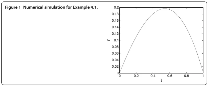
Figure 1 Numerical simulation for Example 4.1.
However, in Theorem ., whether the transcendental equation has a solution is somewhat difficult to verify. It can be seen that each method has its pros and cons.
Example . Consider the BVP
y(t) + (t+ )
y +
= , <t< , (.)
y() = , y() =
y(s)ds+
y(s)ds, (.)
where
a(t) = t+ , f(y) =y
+ , α=
, η=
, α=
, η= .
It is not difficult to see that
aL= , al= , ¯f∞=
, f=∞,
i=
αiηi= . > ,
i=
αiηi < .
In view of sinA
sinA= ., Matlab software givesA= . andA
= .. Hence
¯
f∞= <
A aL <
A
al <f=∞.
Therefore, the condition (ii) of Theorem . is satisfied. A numerical simulation (Figure ) for Example . demonstrates that BVP (.)-(.) has a positive solutiony(t) such that y() = ..
Competing interests
The authors declare that they have no competing interests.
Authors’ contributions
Acknowledgements
The authors would like to thank the editors and the anonymous referees for their valuable suggestions on the improvement of this paper. First author was partially supported by the Scientific Research Fund of Hunan Provincial Educational Department (1200361), Project of Science and Technology Bureau of Hengyang, Hunan Province (2012KJ2). Second author was partially supported by the Doctor Foundation of University of South China ( No. 5-XQD-2006-9), the Foundation of Science and Technology Department of Hunan Province (No. 2009RS3019), the Natural Science Foundation of Hunan Province (No. 13JJ3074) and the Subject Lead Foundation of University of South China (No. 2007XQD13).
Received: 3 March 2013 Accepted: 8 August 2013 Published: 9 September 2013 References
1. Chasreechai, S, Tariboon, J: Positive solutions to generalized second-order three-point boundary value problem. Electron. J. Differ. Equ.14, 1-14 (2011)
2. Gupta, CP: Solvability of a three-point nonlinear boundary value problem for a second order ordinary differential equations. J. Math. Anal. Appl.168, 540-551 (1992)
3. Kwong, MK, Wong, JSW: Some remarks on three-point and four-point BVP’s for second-order nonlinear differential equations. Electron. J. Qual. Theory Differ. Equ.20, 1-18 (2009)
4. Kwong, MK, Wong, JSW: The shooting method and nonhomogeneous multipoint BVPs of second-order ODE. Bound. Value Probl. (2007). doi:10.1155/2007/64012.
5. Li, J, Shen, J: Multiple positive solutions for a second-order three-point boundary value problems. Appl. Math. Comput.182(1), 258-268 (2006)
6. Liu, B, Liu, L, Wu, Y: Positive solutions for singular second order three-point boundary value problems. Nonlinear Anal., Theory Methods Appl.66, 2756-2766 (2007)
7. Ma, R: Positive solutions for second-order three-point boundary value problems. Comput. Math. Appl.40, 193-204 (2000)
8. Ma, R: Positive solutions of a nonlinearm-point boundary value problem. Comput. Math. Appl.42, 755-765 (2001) 9. Tariboon, J, Sitthiwirattham, T: Positive solutions of a nonlinear three-point integral boundary value problem. Bound.
Value Probl. (2010). doi:10.1155/2010/519210
10. Kwong, MK, Wong, JSW: Solvability of second-order nonlinear three-point boundary value problems. Nonlinear Anal.
73, 2343-2352 (2010)
11. Agarwal, RP: The numerical solution of multipoint boundary value problems. J. Comput. Appl. Math.5, 17-24 (1979) 12. Kwong, MK: The shooting method and multiple solutions of two/multi-point BVPS of second-order ODE. Electron. J.
Qual. Theory Differ. Equ.6, 1-14 (2006)
13. You, BL: Supplemental Tutorial of Ordinary Differential Equations. Science Press, Beijing (1987) (in Chinese)
doi:10.1186/1687-2770-2013-205