An Algebraic Approach to Maliciously Secure Private Set
Intersection
Satrajit Ghosh1 and Tobias Nilges2 1
Department of Computer Science, Aarhus University, Denmark 2
ITK Engineering GmbH, Germany
Abstract
Private set intersection is an important area of research and has been the focus of many works over the past decades. It describes the problem of finding an intersection between the input sets of at least two parties without revealing anything about the input sets apart from their intersection.
In this paper, we present a new approach to compute the intersection between sets based on a primitive called Oblivious Linear Function Evaluation (OLE). On an abstract level, we use this primitive to efficiently add two polynomials in a randomized way while preserving the roots of the added polynomials. Setting the roots of the input polynomials to be the elements of the input sets, this directly yields an intersection protocol with optimal asymptotic communication complexityO(mκ). We highlight that the protocol is information-theoretically secure assuming OLE.
We also present a natural generalization of the 2-party protocol for the fully malicious multi-party case. Our protocol does away with expensive (homomorphic) threshold encryption and zero-knowledge proofs. Instead, we use simple combinatorial techniques to ensure the security. As a result we get a UC-secure protocol with asymptotically optimal communication complexity O((n2+nm)κ), wherenis the number of parties,mis the set size andκthe security parameter. Apart from yielding an asymptotic improvement over previous works, our protocols are also conceptually simple and require only simple field arithmetic.
Along the way we develop tools that might be of independent interest.
Keywords: Private set intersection, threshold private set intersection, oblivious linear function evaluation, multi-party, UC-security
1
Introduction
Private set intersection (PSI) has been the focus of research for decades and describes the following basic problem. Two parties, Alice and Bob, each have a set SA and SB, respectively, and want to find the intersectionS∩ =SA∩SB of their sets. This problem is non-trivial if both parties must not
learn anything but the intersection. There are numerous applications for PSI from auctions [NPS99] over advertising [PSSZ15] to proximity testing [NTL+11].
Over the years several techniques for two-party PSI have been proposed, which can be roughly placed in four categories: constructions built from specific number-theoretic assumptions [Sha80, MM87, HFH99, DKT10, DT10], using garbled circuits [HEK12, PSSZ15], based on oblivious trans-fer (OT) [DCW13, PSZ14, PSZ16, OOS17, KKRT16, RR17] and based on oblivious polynomial evaluation (OPE) [FNP04, DMRY09, HN12, Haz15, FHNP16]. There also exists efficient PSI protocols in server-aided model [KMRS14].
Some of these techniques translate to the multi-party setting. The first (passively secure) multi-party PSI (MPSI) protocol was proposed by Freedman et al. [FNP04] based on OPE and later improved in a series of works [KS05, SS08, CJS12] to achieve full malicious security. Recently, Hazay and Venkitasubramaniam [HV17] proposed new protocols secure against semi-honest and fully malicious adversaries. They improve upon the communication efficiency of previous works by designating a central party that runs a version of the protocol of [FNP04] with all other parties and aggregates the results.
Given the state of the art, it remains an open problem to construct a protocol with asymp-totically optimal communication complexity in the fully malicious multi-party setting. The main reason for this is the use of zero-knowledge proofs and expensive checks in previous works, which incur an asymptotic overhead over passively secure solutions.
In a concurrent and independent work, Kolesnikov et al. [KMP+17] presented a new paradigm for solving the problem of MPSI from oblivious programmable pseudorandom functions (OPPRF). Their approach yields very efficient protocols for multi-party PSI, but the construction achieves only passive security againstn−1 corruptions. However, their approach to aggregate the intermediate results uses ideas similar to our masking scheme in the multi-party case.
1.1 Our Contribution
We propose a new approach to (multi-party) private set intersection based on oblivious linear function evaluation (OLE). OLE allows two mutually distrusting parties to evaluate a linear function
ax+b, where the sender knows aand b, and the receiver knows x. Nothing apart from the result
ax+bis learned by the receiver, and the sender learns nothing aboutx. OLE can be instantiated in the OT-hybrid model from a wide range of assumptions with varying communication efficiency, like LPN [ADI+17], Quadratic/Composite Residuosity [IPS09] and Noisy Encodings [IPS09, GNN17], or even unconditionally [IPS09].
Our techniques differ significantly from previous works and follow a new paradigm which leads to conceptually simple and very efficient protocols. This results in asymptotic efficiency improvements over previous works in both communication and computational complexity (cf. Table 1). Our approach is particularly efficient if all input sets are of similar size. To showcase the benefits of our overall approach, we also describe how our MPSI protocol can be modified into a threshold MPSI protocol.
Concretely, we achieve the following:
Protocol Tools Communication Computation Corruptions Security [KMP+17] OPPRF O(nmκ) O(nκ) n−1 semi-honest
[HV17] THE O(nmκ) O(nmlogm) n−1 semi-honest [KS05] THE, ZK O(n2m2κ) O(n2m+nm2κ) n−1 malicious [CJS12] THE, ZK O(n2mκ) O(n2m+nmκ) t < n/2 malicious [HV17] CRS, THE O((n2+nmlogm)κ) O(m2) n−1 malicious Ours+[GNN17] OLE O((n2+nm)κ) O(nmlogm) n−1 malicious1
Table 1: Comparison of multi-party PSI protocols, where n is the number of parties, m the size of the input set and κ a security parameter. The computational cost does not distinguish between exponentiations and multiplications. Some of the protocols perform better if the sizes of the input sets differ significantly, or particular domains for inputs are used. The overhead described here assumes sets of similar size, withκ bit elements.
• UC-secure Multi-party PSI in fully malicious setting with communication complexityO((n2+
nm)κ) and computational complexity O(nmlog2m) for the central party and O(mlog2m) for the other parties.
• A simple extension of the multi-party PSI protocol to threshold PSI, with the same complexity. To the best of our knowledge, this is the first actively secure threshold multi-party PSI protocol.
In comparison to previous works which rely heavily on exponentiations in fields or groups, our protocols require only field addition and multiplication (and OWF in the case of MPSI). We want to emphasize that this efficiency holds including the communication and computation cost for the OLE, if the recent instantiation by Ghosh et al. [GNN17] is used, which is based on noisy Reed-Solomon codes. This OLE protocol has a constant communication overhead and therefore does not influence the asymptotic efficiency of our result. Our results may seem surprising in light of the information-theoretic lower bound of O(n2mκ) in the communication complexity for multi-party PSI in the fully malicious UC setting. We circumvent this lower bound by considering a slightly modified ideal functionality, resulting in a UC-secure solution for multi-party PSI with asymptotically optimal communication overhead. By asymptotically optimal, we mean that our construction matches the optimal bounds in the plain model for m > n, even for passive security, where nis the number of parties, m is the size of the sets andκ is the security parameter. All of our protocols work over fields F that are exponential in the size of the security parameter κ.
We believe that our approach provides an interesting alternative to existing solutions and that the techniques which we developed can find application in other settings as well.
1.2 Technical Overview
Abstractly, we let both parties encode their input set as a polynomial, such that the roots of the polynomials correspond to the inputs. This is a standard technique, but usually the parties then use OPE to obliviously evaluate the polynomials or some form of homomorphic encryption. Instead, we devise an OLE-based construction to add the two polynomials in an oblivious way, which results in an intersection polynomial. Kissner and Song [KS05] also create an intersection polynomial similar to ours, but encrypted under a layer of homomorphic encryption, whereas our technique results in
1
aplain intersection polynomial. Since the intersection polynomial already hides everything but the intersection, one could argue that the layer of encryption in [KS05] incurs additional overhead in terms of expensive computations and complex checks.
In our case, both parties simply evaluate the intersection polynomial on their input sets and check if it evaluates to 0. This construction is information-theoretically secure in the OLE-hybrid model and requires only simple field operations. Conceptually, we compute the complete intersec-tion in one step. In comparison to the naive OPE-based approach2, our solution directly yields an asymptotic communication improvement in the input size. Another advantage is that our approach generalizes to the multi-party setting.
We start with a detailed overview of our constructions and technical challenges.
Oblivious polynomial addition from OLE. Intuitively, OLE is the generalization of OT to larger fields, i.e. it allows a sender and a receiver to compute a linear functionc(x) =ax+b, where the sender holds a, b and the receiver inputs x and obtains c. OLE guarantees that the receiver learns nothing abouta, b except for the resultc, while the sender learns nothing aboutx.
Based on this primitive, we define and realize a functionality OPA that allows to add two polynomials in such a way that the receiver cannot learn the sender’s input polynomial, while the sender learns nothing about the receiver’s polynomial or the output. We first describe a passively secure protocol. Concretely, assume that the sender has an input polynomialaof degree 2d, and the receiver has a polynomial b of degree d. The sender additionally draws a uniformly random polynomial r of degree d. Both parties point-wise add and multiply their polynomials, i.e. they evaluate their polynomials over a set of 2d+ 1 distinct points α1, . . . , α2d+1, resulting in ai = a(αi), bi =b(αi) and ri = r(αi) for i∈ [2d+ 1]. Then, for each of 2d+ 1 OLEs, the sender inputsri, ai, while the receiver inputsbi and thereby obtainsci =ribi+ai. The receiver interpolates the polynomialc from the 2d+ 1 (αi, ci) and outputs it. Since we assume semi-honest behaviour,
the functionality is realized by this protocol.
The biggest hurdle in achieving active security for the above protocol lies in ensuring non-zerob
andr. In particular, the protocol has to ensure that the inputsbandrare non-zero. Otherwise, e.g. ifb= 0, the receiver could learna. One might think that it is sufficient to perform a coin-toss and verify that the output satisfies the supposed relation, i.e. pick a randomx, computea(x), b(x), r(x) andc(x) and everyone checks ifb(x)r(x) +a(x) =c(x) and ifb(x), r(x) are non-zero. Forr(x)6= 0, the check is actually sufficient, becauser must have degree at mostd, otherwise the reconstruction fails, and only d points of r can be zero (r = 0 would require 2d+ 1 zero inputs). For b 6= 0, however, just checking forb(x)6= 0 is not sufficient, because at this point, even if the inputb6= 0, the receiver can input d zeroes in the OLE, which in combination with the check is sufficient to learn a completely. We resolve this issue by constructing an enhanced OLE functionality which ensures that the receiver input is non-zero. We believe that this primitive is of independent interest and describe it in more detail later in this section.
Two-party PSI from OLE. Let us first describe a straightforward two-party PSI protocol with one-sided output from the above primitive. Let SA and SB denote the inputs for Alice and Bob, respectively, where |SP|=m. They computepA and pB such that pP(γ) = 0 for γ ∈SP. If
Bob is supposed to get the intersection, Alice picks a uniformly random polynomialrA of degreem
and inputspA,rA into OPA. Bob inputs pB, obtainsp∩ =pA+pBrA and outputs allγj ∈SB for
which p∩(γj) = 0. Obviously, rA does not remove any of the roots of pB, and therefore all points
2
γ wherepB(γ) = 0 =pA(γ) remain in p∩.
However, as a stepping stone for multi-party PSI, we are more interested in protocols that provide output to both parties. If we were to use the above protocol and simply announce p∩ to Alice, then Alice could learn Bob’s input. Therefore we have to take a slightly different approach. LetuA be an additional random polynomial chosen by Alice. Instead of using her own input in the OPA, Alice uses rA,uA, which gives sB =uA+pBrA to Bob. Then they run another OPA in the
other direction, i.e. Bob inputsrB,uB and AlicepA. Now, both Alice and Bob have a randomized “share” of the intersection, namely sA and sB, respectively. Adding sA and sB yields a masked but correct intersection. We still run into the problem that sending either sB to Alice or sA to
Bob allows the respective party to learn the other party’s input. We also have to use additional randomization polynomialsr0A,r0B to ensure privacy of the final result.
Our solution is to simply use the masks u to enforce the addition of the two shares. Let us fix Alice as the party that combines the result. Bob computes s0B =sB−uB +pBr0B and sends it to Alice. Alice computes p∩ =s0B+sA −uA+pAr
0
A. This way, the only chance to get rid of the
blinding polynomialuB is to add both values. But since each input is additionally randomized via
the rpolynomials, Alice cannot subtract her own input from the sum. Since the same also holds for Bob, Alice simply sends the result to Bob.
The last step is to check if the values that are sent and the intersection polynomial are consistent. We do this via a simple coin-toss for a randomx, and the parties evaluate their inputs onxand can abort if the relationp∩ =pB(rA+r
0
B) +pA(r 0
A+rB) does not hold, i.e. p∩ is computed incorrectly. This type of check enforces semi-honest behaviour, and was used previously e.g. in [BFO12].
A note on the MPSI functionality. We show that by slightly modifying the ideal func-tionality for multi-party PSI we get better communication efficiency, without compromising the security at all. A formal definition is given in Section 6.1. Typically, it is necessary for the sim-ulator to extract all inputs from the malicious parties, input them into the ideal functionality, and then continue the simulation with the obtained ideal intersection. In a fully malicious setting, however, this requires every party to communicate in O(mκ) with every other party—otherwise the input is information-theoretically undetermined and cannot be extracted—which results in
O(n2mκ) communication complexity.
The crucial observation here is that in the setting of multi-party PSI, an intermediate intersec-tion between a single malicious party andall honest parties is sufficient for simulation. This is due to the fact that inputs by additional malicious parties can only reduce the size of the intersection, and as long as we observe the additional inputs at some point, we can correctly reduce the inter-section in the ideal setting before outputting it. On a technical level, we no longer need to extract all malicious inputs right away to provide a correct simulation of the intersection. Therefore, it is not necessary for every party to communicate in O(mκ) with every other party. Intuitively, the intermediate intersection corresponds to the case where all malicious parties have the same input. We therefore argue that the security of this modified setting is identical to standard MPSI up to input substitution of the adversary.
their intersection with the central party.
First, consider the following (incorrect) toy example. Let each party Pi execute the two-party PSI as described above with P0, up to the point where both parties have shares siP0,s
0
Pi. All parties Pi send their shares s0P
i to P0, who adds all polynomials and broadcasts the output. By design of the protocols and the inputs, this yields the intersection of all parties. Further, the communication complexity is in O(nmκ), which is optimal. However, this protocol also allowsP0
to learn all intermediate intersections with the other parties, which is not allowed. Previously, all maliciously secure multi-party PSI protocols used threshold encryption to solve this problem, and indeed it might be possible to use a similar approach to ensure active security for the above protocol. For example, a homomorphic threshold encryption would allow to add all these shares homomorphically, without leaking the intermediate intersections. But threshold encryption incurs a significant computational overhead (and increases the complexity of the protocol and its analysis) which we are unwilling to pay.
Instead, we propose a new solution which is conceptually very simple. We add another layer of masking on the sharessPi, which forces P0 to addall intermediate shares—at least those of the honest parties. For this we have to ensure that the communication complexity does not increase, so all parties exchange seeds (instead of sending random polynomials directly), which are used in a PRG to mask the intermediate intersections. This technique is somewhat reminiscent of the pseudorandom secret-sharing technique by Cramer et al. [CDI05]. We emphasize that we do not need any public key operations.
Concretely, all parties exchange a random seed and use it to compute a random polynomial in such a way that every pair of parties Pi, Pj holds two polynomials vij,vji with vij +vji = 0. Then, instead of sending s0Pi, each party Pi computes s00Pi = s0Pi +P
vij and sends this value. If
P0 obtains this value, it has to add the valuess00P
i of all parties to remove the masks, otherwise s
00 Pi will be uniformly random.
Finally, to ensure that the central party actually computed the aggregation, we add a check similar to two-pary PSI, where the relation, i.e. computing the sum, is verified by evaluating the inputs on a random value x which is obtained by a multi-party coin-toss.
Threshold (M)PSI. First of all, we clarify the term threshold PSI. We consider the setting where all parties havem elements as their input, and the output is only revealed if the intersection of the inputs among all parties is bigger than a certain threshold `. In [HOS17] Hallgren et al. defined this notion for two party setting, and finds application whenever two entities are supposed to be matched once a certain threshold is reached, e.g. for dating websites or ride sharing. In contrast, Kissner and Song [KS05] previously defined an over-threshold PSI protocol, where an element appears in the intersection if the number of occurrences of this element among the n
parties is bigger than the threshold.
We naturally extend the idea of threshold PSI from [HOS17] to a multi-party settings and propose the first actively secure threshold multi-party PSI protocol. On a high level, our solution uses a similar idea to [HOS17], but we use completely different techniques and achieve stronger security and better efficiency. The main idea is to use a robust secret sharing scheme, and the execution of the protocol basically transfers a subset of these shares to the other parties, one share for each element in the intersection. If the intersection is large enough, the parties can reconstruct the shared value.
pi(γj) = 1. Further, for each of the random polynomialsri,r0i we setri(γj) =ρj and r0i(γj) =ρ0j, where ρ1, . . . , ρn, ρ01, . . . , ρ0n are the shares of two robust (`, n)-secret sharings of random values
s0i and s1i, respectively. Now, by computing the intersection polynomial p∩ as before, each party obtains exactly m∩ =|S∩|shares, one for eachγj ∈Si. If m∩ ≥`then each party can reconstruct
r∩ = Pni=1(s 0
i +s1i), otherwise the intersection remains hidden completely. Given a successful
reconstruction, the set S∩ can be easily identified by using the locations γj of valid shares in p∩. We believe that our techniques can also be applied to [KS05] or follow-up works, but due to the use of threshold homomorphic encryption and zero-knowledge proofs, the efficiency of these protocols would be inferior to our solution.
A New Flavour of OLE. One of the main technical challenges in constructing our protocols is to ensure a non-zero input into the OLE functionality by the receiver. Recall that an OLE computes a linear functionax+b. We define an enhanced OLE functionality (cf. Section 3) which ensures that x 6= 0, otherwise the output is uniformly random. Our protocol which realises this functionality makes two black-box calls to a normal OLE and is otherwise purely algebraic.
Before we describe the solution, let us start with a simple observation. If the receiver inputs
x = 0, an OLE returns the value b. Therefore, it is critical that the receiver cannot force the protocol to output b. One way to achieve this is by forcing the receiver to multiply b with some correlated value via an OLE, lets call it ˆx. Concretely, we can use an OLE where the receiver inputs ˆ
xand a randoms, while the sender inputsband obtains ˆxb+s. Now if the sender usesa+bxˆ+s,0 as input for another OLE, where the receiver inputsx, the receiver obtainsax+bxxˆ +sx. Which means that if ˆx =x−1 then the receiver can extract the correct output. This looks like a step in the right direction, since for x = 0 or ˆx = 0, the output would not be b. On the other hand, the receiver can now force the OLE to outputaby choosing ˆx= 0 andx= 1, so maybe we only shifted the problem.
The final trick lies in masking the output such that it is uniform for inconsistent inputsx,xˆ. We do this by splittingbinto two shares that only add tobifx·xˆ= 1. The complete protocol looks like this: the receiver plays the sender for one OLE with inputx−1, s, and the sender inputs a randomu
to obtaint=x−1u+s. Then the sender plays the sender for the second OLE and inputst+a, b−u, while the receiver inputsxand obtainsc0 = (t+a)x+b−u=ux−1x+sx+ax+b−u=ax+b+sx, from which the receiver can subtract sx to get the result. A cheating receiver with inconsistent input x∗,xˆ∗ will getax+b+u(x∗xˆ∗−1) as an output, which is uniform over the choice ofu.
1.3 Structure of the Paper
We start with the definition and construction of the enhanced OLE functionality in Section 3. In Section 4 we define an ideal functionality for the addition of polynomials and describe a protocol that realizes this functionality black-box from OLE. Based on this primitive, we first provide a two-party PSI protocol in Section 5 and later a multi-party PSI protocol in Section 6.
2
Preliminaries
In the proofs, ˆx denotes an element either extracted or simulated by the simulator, while x∗
denotes an element sent by the adversary.
We slightly abuse notation and denote by v=PRGd(s) the deterministic pseudorandom
poly-nomial of degreedderived from evaluating PRGon seeds.
2.1 Security Model
We prove our protocol in the Universal Composability (UC) framework of Canetti [Can01]. In the framework, security of a protocol is shown by comparing a real protocol π in the real world with an ideal functionality F in the ideal world. F is supposed to accurately describe the security requirements of the protocol and is secure per definition. An environmentZis plugged either to the real protocol or the ideal protocol and has to distinguish the two cases. For this, the environment can corrupt parties. To ensure security, there has to exist a simulator in the ideal world that produces a protocol transcript indistinguishable from the real protocol, even if the environment corrupts a party. We say π UC-realises F if for all adversaries A in the real world there exists a simulator S in the ideal world such that all environments Z cannot distinguish the transcripts of the parties’ outputs.
Oblivious Linear Function Evaluation. Oblivious Linear Function Evaluation (OLE) is a special case of Oblivious Polynomial Evaluation (OPE). In contrast to OPE, only linear functions can be obliviously evaluated. The sender has as input two values a, b∈F that determine a linear functionf(x) =a·x+boverF, and the receiver gets to obliviously evaluate the linear function on input x∈F. The receiver will learn onlyf(x), and the sender learns nothing at all. Consider the ideal functionality in Figure 1.
FunctionalityFOLE
1. Upon receiving a message (inputS,(a, b)) from the sender witha, b∈F, verify that there is no stored
tuple, else ignore that message. Storeaandb and send a message (input) toA.
2. Upon receiving a message (inputR, x) from the receiver withx∈ F, verify that there is no stored
tuple, else ignore that message. Storexand send a message (input) toA.
3. Upon receiving a message (deliver,S) fromA, check if both (a, b) andxare stored, else ignore that message. Send (delivered) to the sender.
4. Upon receiving a message (deliver,R) fromA, check if both (a, b) andxare stored, else ignore that message. Sety=a·x+b and send (output, y) to the receiver.
Figure 1: Ideal functionality for oblivious linear function evaluation.
To instantiate our PSI protocol we choose an efficient batch-OLE protocol based on Noisy Reed-Solomon-Codes from [GNN17]. The protocol has a constant communication overhead of 64 field elements per OLE, and require onlyO(logm) simple field operations, whereκ-bit prime field gives
κ-bit security.
2.2 Commitment from FOLE
queries with a random x, we get a UC-secure commitment. Intuitively, the commitment can be simulated because the simulator knows x and can adjust r, and it can be extracted because the simulator learns the message as an input.
The above commitment protocol, however, does not realise FmCOM. In order to do so, we have to include the id of the sender pid to prevent man-in-the-middle attacks, in particular copying of the commitment. Interestingly, this poses a difficulty in theFOLE-hybrid setting, since our message space is limited. So either we pick a larger fieldF0 such that we can embed inm0∈F0 both m∈F andpid, or we directly construct a commitment which has a slightly larger message space. We take the second approach in Figure 2.
Protocol ΠmCOM
Letpid∈F denote the ID of partyPi.
Commit Phase
1. Party Pi (Input m ∈ F): Choose a random r1, r2 ∈ F. Input (inputS,(m, r1)) into F (0) OLE and
(inputS,(m·pid, r2)) intoFOLE(1) .
2. Party Pj: Choose random x, y ∈ F. Input (inputR, x) into F
(0)
OLE and (inputR, y) into F (1) OLE to
obtainq1, q2.
Unveil Phase
3. PartyPi: Send (m, r1, r2) toPj.
4. PartyPj: Accept ifq1=m·x+r1andq2=m·pid·y+r2, abort otherwise.
Figure 2: ΠmCOM in theFOLE-hybrid model.
Lemma 1. The protocol ΠmCOM UC-realizes FmCOM in the FOLE-hybrid model.
Sketch. CorruptedPi. The simulator against the committing party observes ˆm,mˆ0and alsor1, r2. It aborts ifγ = ˆm0/mˆ 6=pid forPi. Otherwise, it sends (commit, Pi, Pj,mˆ) to FmCOM.
Let (α, β1, β2) denote the unveil. This simulation is indistinguishable from the real protocol,
since the check of the unveil will always fail ifα6= ˆm. Letσ denote the outcome of the check from A’s view.
σ=αx+β1−q1 = (α−mˆ)x+β1−r1.
Thus, from A’s view,σ is uniform over the choice ofx. We now know thatα= ˆm. Ifγ 6=pid,
σ0 = ˆm·pidy+β2−q2= ( ˆm·pid−mˆ ·γ)y+β2−r2.
In this case, σ0 is uniform over the choice of y and the protocol would abort. In conclusion, the simulator extracts the right input and provides an indistinguishable simulation of the real protocol.
Corrupted Pj. The simulator against the receiving party observes the challenges ˆx,yˆ and simulates the commit phase with a random input ρ using randomness r1, r2. Upon receiving a
2.3 Non-malleable Commitments
Roughly, the setting of concurrent non-malleable commitments is as follows. An adversary MIM
interacts in a left session with polynomially many committers, while simultaneously interacting with receivers inm right sessions. We denote byMIMmCOM(v, z) the distribution of all values committed
by MIM in the right sessions, and SimmCOM(1κ, z) the joint distribution of all values committed by the simulator.
Definition 2. A commitment scheme{COM.Commit,COM.Open}is said to bem-bounded-concurrent non-malleable if for every PPT MIM, there exists a PPT simulator S such that the following en-sembles are computationally indistinguishable:
{MIMmCOM({v}, z)}κ∈
N,v∈{0,1}κ,z∈{0,1}∗ and {Sim
m
COM(1κ, z)}κ∈N,v∈{0,1}κ,z∈{0,1}∗
2.4 Technical Lemmas
We state several lemmata which are used to show the correctness of our PSI protocols later on.
Lemma 3. Let p,q∈F[X]be non-trivial polynomials. Then,
M0(p)∩ M0(p+q) =M0(p)∩ M0(q) =M0(q)∩ M0(p+q).
This lemma shows that the sum of two polynomials contains the intersection with respect to the zero-sets of both polynomials.
Proof. Let M∩ =M0(p)∩ M0(q).
“⊇00: ∀x∈ M∩: p(x) =q(x) = 0. But p(x) +q(x) = 0, so x∈ M0(p+q).
“ ⊆00: It remains to show that there is no x such that x∈ M0(p)∩ M0(p+q) but x /∈ M∩, i.e.M0(p)∩(M0(p+q)\ M∩) =∅. Similarly, M0(q)∩(M0(p+q)\ M∩) =∅.
Assume for the sake of contradiction that M0(p)∩(M0(p+q)\ M∩)6=∅. Let x∈ M0(p)∩ (M0(p +q)\ M∩). Then, p(x) = 0, but q(x) 6= 0, otherwise x ∈ M∩. But this means that
p(x) +q(x) 6= 0, i.e.x /∈ M0(p+q). This contradicts our assumption, and we get that M0(p)∩ (M0(p+q)\ M∩) =∅.
Symmetrically, we get that M0(q)∩(M0(p+q)\ M∩) =∅. The claim follows.
Lemma 4. Let d ∈ poly(log|F|). Let p ∈ F[X], deg(p) = d be a fixed but unknown non-trivial polynomial. Further let q1, . . . ,ql∈F[X] withdeg(qi)≤d.
Pr
p∈F[X]
[(M0(p)∩ M0(
l X
i=1
qi))6= (M0(p)∩
l \
i=1
M0(qi))]≤negl(|F|).
This lemma is basically an extension of Lemma 3 and shows that the sum of several polynomials does not create new elements in the intersection unless the supposedly unknown zero-set ofp can be guessed with non-negligible probability.
Proof. We first observe that Tli=1M0(qi)⊆ M0(Pli=1qi): it holds that for all x∈Tli=1M0(qi),
Now, assume for the sake of contradiction that
(M0(p)∩ M0(
l X
i=1
qi))6= (M0(p)∩
l \
i=1
M0(qi))
with non-negligible probability . LetM=M0(Pli=1qi)\Tli=1M0(qi).
Then with probability at least , the set M is not empty. Further, we can bound |M| ≤ d. Pick a random x ∈ M. It holds that Pr[x ∈ M0(p)] ≥ /d, which is non-negligible. But since
p is unknown, so is M0(p), and the probability that we can find x, so that x ∈ M0(p) is upper bounded by d/|F|overp.
This is a contradiction and the claim follows.
Lemma 5. Let d, d0 ∈poly(log|F|). Let r∈F[X], deg(r) =d be a uniformly random polynomial.
For all non-trivial p∈F[X], deg(p) =d0,
Pr
r∈F[X]
[(M0(r)∩ M0(p))6=∅]≤negl(|F|).
This lemma establishes that the intersection of a random polynomial with another polynomial is empty except with negligible probability.
Proof. This follows from the fundamental theorem of algebra, which states that a polynomial of degree devaluates to 0 in a random point only with probabilityd/|F|.
Sincer(and therefore allx∈ M0(r)) is uniformly random and|M0(r)|=d, while|M0(p)|=d0, we get that
Pr[(M0(r)∩ M0(p))6=∅]≤dd0/|F|.
Lemma 6. Let d ∈ poly(log|F|). Let p ∈ F[X], deg(p) = d be a fixed but unknown non-trivial polynomial. Further letr∈F[X],deg(r) =dbe a uniformly random polynomial. For all non-trivial q,s∈F[X]with deg(q)≤dand deg(s)≤d,
Pr
r∈F[X][(
M0(p)∩ M0(ps+rq))6= (M0(p)∩ M0(q))]≤negl(|F|).
This lemma shows that the multiplication of (possibly maliciously chosen) polynomials does not affect the intersection except with negligible probability, if one random polynomial is used.
Proof.
M0(p)∩ M0(ps+rq) Lemma= 3 M0(p)∩(M0(ps)∩ M0(qr))
= M0(p)∩ (M0(p)∪ M0(s))∩(M0(q)∪ M0(r))
= M0(p)∩ (M0(p)∩ M0(q))∪(M0(p)∩ M0(r)
| {z }
T1
)
∪(M0(s)∩ M0(q)
| {z }
⊆M0(q)
)∪(M0(s)∩ M0(r)
| {z }
T2
From Lemma 5 it follows that Pr[T1 6=∅]≤d2/|F|, and also Pr[T26=∅]≤d2/|F|. Since
M0(p)∩ (M0(p)∩ M0(q))∪ M0(q)=M0(p)∩ M0(q),
we get
Pr
r∈F[X][(
M0(p)∩ M0(ps+rq))6= (M0(p)∩ M0(q))]≤2d2/|F|.
3
Enhanced Oblivious Linear Function Evaluation
F
OLE+In this section we present an enhanced version of the OLE functionality. The standard OLE functionality allows the sender to inputa, b, while the receiver inputsxand obtainsax+b. For our applications, we do not want the receiver to be able to learn b, i.e. it has to hold that x6= 0. Our approach is therefore to modify the OLE functionality in such a way that it outputs a random field element upon receiving an input x = 0 (cf. Figure 3). A different approach might be to output a special abort symbol or 0, but crucially the output must not satisfy the relation ax+b. This is a particularly useful feature, as we will show in the next section.
FOLE+
1. Upon receiving a message (inputS,(a, b)) from the sender witha, b∈F, verify that there is no stored
tuple, else ignore that message. Otherwise, store (a, b) and send (input) toA.
2. Upon receiving a message (inputR, x) from the receiver withx∈ F, verify that there is no stored
value, else ignore that message. Otherwise, storexand send (input) toA.
3. Upon receiving a message (deliver) from A, check if both (a, b) andxare stored, else ignore that message. Ifx6= 0, setc=ax+b, otherwise pick a uniformly randomc∈F and send (output, c) to
the receiver. Ignore all further messages.
Figure 3: Ideal functionality for the enhanced oblivious linear function evaluation.
While it might be possible to modify existing OLE protocols in such a way that a non-zero input is guaranteed, we instead opt to build a protocol black-box from the standard OLE functionality FOLE.
Let us begin with a short overview of our construction. Our main goal is to prevent leakage of the value b on input x = 0. One way to ensure that is by using an OLE and computing xb. However, the result of the enhanced OLE should still beax+bforx6= 0. Thus, we have to remove the connection of x and b with a second OLE, while at the same time adding another connection with a. The key idea is to force the receiver to use x−1 and x as his inputs, thus cancelling the relation betweenx and bif the inputs were chosen correctly.
Concretely, one first attempt might be to execute an OLE from receiver to sender, where the receiver inputsx−1 and a random value s. The sender inputs band obtains bx−1+s, then addsa
and uses (bx−1+a+s,0) for the second OLE. The receiver inputsxand thereby obtainsax+b+sx
from which he can subtractsx(because he knows both sand x) and output c=ax+b.
not be allowed. Therefore, we make a small modification to the above described protocol. Instead of sending b to the first OLE, the sender picks a uniformly random u and obtains ux−1+s. In order to still get the correct result, the senders input into the second OLE has to be changed to (ux−1+a+s, b−u). If the receiver cheats with his inputs, the term u will completely randomize the output, since c = ax+b+uxx−1−u+sx. The formal description of the protocol is given in Figure 4.
ΠOLE+
1. Receiver (Inputx∈F): Picks∈F and send (inputS,(x−1, s)) to the firstFOLE.
2. Sender (Inputa, b∈F): Pick u∈F uniformly at random and send (inputR, u) to the firstFOLE to
learnt=ux−1+s. Send (inputS,(t+a, b−u)) to the secondFOLE.
3. Receiver: Send (inputR, x) to the secondFOLE and obtainc=ax+b+sx. Outputc−sx.
Figure 4: Protocol that realizes F
OLE+ in the FOLE-hybrid model.
Lemma 7. ΠOLE+ unconditionally UC-realizes F
OLE+ in the FOLE-hybrid model.
Proof. The simulator against a corrupted sender simulates both instances of FOLE. Let α1 be the
sender’s input in the first OLE, and (α2, α3) be the inputs into the second OLE. The simulator sets ˆb=α1+α3 and ˆa=α2−ˆt, where ˆt is chosen as the uniformly random output to AS of the first OLE. The simulator simply inputs (inputS,(ˆa,ˆb)) intoF
OLE+. Let us briefly argue that this
simulation is indistinguishable from a real protocol run. The value ˆt is indistinguishable from a valid t, since the receiver basically uses a one-time-pad s to mask the multiplication. Therefore, the sender can only change his inputs into the OLEs. Since his inputs uniquely determine both ˆa
and ˆb, the extraction by the simulator is correct and the simulation is indistinguishable from a real protocol run.
Against a corrupted receiver, the simulator simulates the two instance of FOLE and obtains the receiver’s inputs (ξ1, ξ3) and ξ2. If ξ1·ξ2 = 1, the simulator sets ˆx = ξ2, sends (inputR,xˆ) to F
OLE+ and receives (output, c). It forwards c
0
=c+ξ2ξ3 to AR. If ξ1·ξ2 6= 1, the simulator
sends (inputR,0) toF
OLE+ and forwards the outputcto the receiver. It remains to argue that this
simulation is indistinguishable from the real protocol. From A’s view, the output c is determined as
c=uξ1ξ2+aξ2+b−u+ξ2ξ3 =aξ2+b+u(ξ1ξ2−1) +ξ2ξ3.
We can ignore the last term, since it is known to A. If ξ1ξ2 = 1, then6 u(ξ1ξ2−1) does not vanish and the result will be uniform over the choice ofu. Thus, by usingξ2 as the correct input otherwise, we extract the correct value and the simulation is indistinguishable from the real protocol.
4
Randomized Polynomial Addition from OLE
this privacy property by using a randomization polynomial that prevents the receiving party from simply subtracting its input from the result. This functionality is defined in Figure 5.
Notice that we have some additional requirements regarding the inputs of the parties. First, the degree of the inputs has to be checked, but the functionality also makes sure that the receiver does not input a 0 polynomial, because otherwise he might learn the input of the sender. Also note that the functionality leaks some information about the sender’s polynomial. Looking ahead in the PSI protocol, where the input of the sender is always a uniformly random 2d degree polynomial, this leakage of the ideal functionality will not leak any non-trivial information in the PSI protocol.
FOPA
Implicitly parameterized bydsignifying the maximal input degree.
1. Upon receiving a message (inputS,(a,r)) from the sender wherea,r∈F[X], check whether • r6= 0
• deg(r)≤dand deg(a) = 2dOR deg(r) =dand deg(a)≤2d and ignore that message if not. Store (a,r) and send (input) toA.
2. Upon receiving a message (inputR,b) from the receiver whereb∈F[X], check whether deg(b)≤d
and b6= 0. If not, ignore that message. Otherwise, retrieve a,r, compute s= r·b+a and send (res,s) to the receiver. Ignore all further messages.
Figure 5: Ideal functionality that allows to obliviously compute an addition of polynomials.
4.1 Passively Secure Protocol for FOPA
It is instructive to first consider a passively secure protocol. In the semi-honest case, both sender and receiver evaluate their input polynomials on a set of distinct points P = {α1, . . . , α2d+1},
wheredis the degree of the input polynomials. The sender additionally picks a random polynomial
r∈F[X] of degreedand also evaluates it on P.
Instead of using OLE in the “traditional” sense, i.e. instead of computingab+rwhererblinds the multiplication of the polynomials, we basically compute rb+a. This means that the sender randomizes the polynomial of the receiver, and then adds his own polynomial. This prevents the receiver from simply subtracting his input polynomial and learninga. In a little more detail, sender and receiver use 2d+ 1 OLEs to add the polynomials as follows: for each i∈[2d+ 1], the sender inputs (ri, ai) in OLEi, while the receiver inputsbi and obtainssi =ribi+ai. He then interpolates the resulting polynomials of degree 2dusing the 2d+ 1 valuessi. The above protocol is described in Figure 6.
Due to the security guarantees of OLE, the sender learns nothing about the result, while the receiver’s input is randomized byr, i.e. he is not able to reconstruct a.
Lemma 8. ΠshOPA UC-realizesFOPA with passive security in the FOLE-hybrid model.
ΠshOPA
LetP ={α1, . . . , α2d+1}, αi∈F be a set of distinct points.
1. Sender (Input a ∈F[X], deg(a) = 2d): Pick r∈ F[X] of degree duniformly at random. Evaluate
a,ronP to obtain (ai, ri), i∈[2d+ 1]. Input (ri, ai) intoF
(i) OLE.
2. Receiver (Input b∈F[X], deg(b) =d): EvaluatebonP and obtain bi, i∈[2d+ 1]. Input bi into
FOLE(i) and receivesi=ribi+ai. Reconstructsfrom thesi and outputs
Figure 6: Protocol that realizes FOPA in theFOLE-hybrid model with passive security.
input. This follows from the fundamental theorem of algebra: we evaluate b in 2d+ 1 distinct points independent of b, and b has exactly droots. The probability that a root is contained inP is therefore (2d+ 1)·d/|F|, which is negligible in|F|.
4.2 Actively Secure Protocol for FOPA
In going from passive to active security, we have to ensure that the inputs of the parties are correct. Here, the main difficulty obviously lies in checking for b = 0. In fact, since FOPA does not even leak a single pointai we have to make sure that all bi6= 0. However, this can easily be achieved by
using F
OLE+ instead of FOLE. We also have to verify that the inputs are well-formed via a simple
polynomial check. For a more detailed overview we refer the reader to the introduction. The complete actively secure protocol is shown in Figure 7.
ΠOPA
LetP ={α1, . . . , α2d+1}, αi∈F be a set of distinct points.
1. Sender (Inputa,r∈F[X], deg(a)≤2d,deg(r) =d): Evaluatea,ronP to obtain (ai, ri), i∈[2d+1]. Input (ri, ai) intoF
(i) OLE+.
2. Receiver (Input b∈F[X], deg(b)≤d): EvaluatebonP and obtain bi, i∈[2d+ 1]. Input bi into
F(i)
OLE+ and receivesi =ai+bi·ri. Reconstructs from thesi and check if deg(s) = 2d, otherwise
abort.
3. Sender: Pick a random xS∈F and send it to the receiver.
4. Receiver: Compute b(xS),s(xS) and pick a randomxR∈F. Send (b(xS),s(xS), xR) to the sender.
5. Sender: Ifs(xS)6=a(xS) +b(xS)·r(xS), abort. Send (a(xR),r(xR)) to the receiver.
6. Receiver: Ifs(xR)6=a(xR) +b(xR)·r(xR) orr(xR) = 0 ora(xR) = 0, abort, otherwise outputs.
Figure 7: Protocol that realizes FOPA in theF
OLE+-hybrid model.
Lemma 9. ΠOPA unconditionally UC-realizesFOPA in the FOLE+-hybrid model.
Proof. Corrupted Sender. The simulatorSS against a corrupted sender proceeds as follows. It simulates F(i)
OLE+ and thereby obtains (r
∗ i, a
∗
reconstructs ˆr and ˆa. It aborts in Step 6 if deg(ˆr)> d or deg(ˆa)>2d. It also aborts if ˆaor ˆrare zero, and otherwise sends (inputS,(ˆa,ˆr)) to FOPA.
The extraction of the corrupted sender’s inputs is correct if his inputs r∗ corresponds to a polynomial of degreedanda∗ corresponds to a polynomial of degree 2d. Thus, the only possibility for an environment to distinguish between the simulation and the real protocol is by succeeding in answering the check while using a malformed input, i.e. a polynomial of incorrect degree or 0-polynomials. If the polynomials have degree greater than d and 2d, respectively, the resulting polynomial s has degree 2d+ 1 instead of 2d, i.e. the receiver cannot reconstruct the result from 2d+ 1 points. Since the sender learns nothing about the receiver’s inputs, the thus incorrectly reconstructed polynomial will be uniformly random from his point of view and the probability that his response to the challenge is correct is 1/|F|. Also, both ˆa and ˆr have to be non-zero, because in each case the polynomials are evaluated in 2d+ 1 points, and it requires 2d+ 1 zeros as ai, ri
to get a 0 polynomial. But since both a,r have degree at most 2d, there are at most 2d roots of these polynomials. Therefore, in order to pass the check,a(x) andb(x) would need to be 0, which is also checked for.
Corrupted Receiver. The simulator SR against a corrupted receiver simulates F(i)
OLE+ and
obtainsb∗i for all i∈[2d+ 1]. It reconstructs ˆb and aborts the check in Step 5 if deg(ˆb)> d. The simulator sends (inputR,bˆ) to FOPA and receives (res,ˆs). It evaluates ˆs on P and returns si for
the corresponding OLEs. SR simulates the rest according to the protocol.
Clearly, if the corrupted receiver AR inputs a degree d polynomial, the simulator will extract the correct polynomial. In order to distinguish the simulation from the real protocol, the adversary can either input 0 in an OLE or has to input a polynomial of higher degree, while still passing the check. In the first case, assume w.l.o.g. that AR cheats inF(j)
OLE+ for some j. This means AR
receives a value ˆsi, which is uniformly random. This means that only with probability 1/|F| will ˆ
si satisfy the relationrb+a and the check will fail. In the second case, the resulting polynomial would be of degree 2d+ 1, while the receiver only gets 2d+ 1 points of the polynomial. Therefore the real polynomial is underdetermined andA can only guess the correct value ˆs(x), i.e. the check will fail with overwhelming probability.
Remark. We use the abstraction ofFOPAto modularize the construction of our PSI protocols. For practical purposes it is possible to remove the check in ΠOPA, since this check only ensures that the inputs and output of the protocol are well-formed polynomials and this can also be checked directly in the PSI protocols.
5
Maliciously Secure Two-party PSI
In this section we provide a maliciously secure two-party PSI protocol with output forboth parties, i.e. we realizeFPSI as described in Figure 8.
FPSI
1. Upon receiving a message (input, P, SP) from party P ∈ {A,B}, store the setSP. Once all inputs are given, setS∩=SA∩SB and send (output, S∩) toA.
2. Upon receiving a message (deliver) fromA, send (output, S∩) to the honest party.
Figure 8: Ideal functionalityFPSI for two-party PSI.
behaviour, and no computational primitives. A formal description is given in Figure 9.
Π2PSI
Letm= maxi|Si|+ 1.
Computation of Intersection
1. Alice (Input SA): Compute a polynomial pA of degree m such that pA(γj) = 0 for all γj ∈ SA. Generate two random polynomialsrA,r
0
A of degreemand a random polynomialuA of degree 2m. • InputrA,uA intoF
(1) OPA. • InputpA intoF
(2)
OPA and obtainsA=pArB+uB. • Sets0A=sA−uA+pAr
0
A and send it to Bob.
2. PB(InputSB): Compute a polynomialpBof degreemsuch thatpB(γj) = 0 for allγj∈SB. Generate
two random polynomialsrB,r 0
B of degreemand a random polynomialuB of degree 2m. • InputrB,uB intoF
(2) OPA. • InputpB intoF
(1)
OPA and obtainsB=pBrA+uA. • Upon receivings0A, computep∩=s0A+sB+pBr 0
B−uB and send it to Alice.
Output Verification
3. Alice: Pick a randomxA∈F and send it to Bob.
4. Bob: Set αB = pB(xA), βB = rB(xA) and δB = r0B(xA). Pick a random xB ∈ F and send (xB, αB, βB, δB) to Alice.
5. Alice: Check ifpA(xA)(βB+r 0
A(xA)) +αB(rA(xA) +δB) =p∩(xA), otherwise abort. For eachγj∈SA:
Ifp∩(γj) = 0, add γj toS∩. SendαA=pA(xB),βA =rA(xB) andδA=r 0
A(xB) to Bob. Output S∩.
6. Bob: Check ifαA(rB(xB) +δA) +pB(xB)(βA+r 0
B(xB)) =p∩(xB), otherwise abort. For eachγj∈SB:
Ifp∩(γj) = 0, add γj toS∩. OutputS∩.
Figure 9: Protocol Π2PSIUC-realises FPSI in theFOPA-hybrid model.
Theorem 1. The protocol Π2PSI UC-realises FPSI in the FOPA-hybrid model with communication complexityO(mκ).
Proof. Let us argue that p∩ = pA(r 0
A+rB) +pB(rA +r 0
B) actually hides the inputs. The main
validly encodes the intersection (see Lemma 3), p∩ is uniformly random over the choice of the randomization polynomialsrA,r0A,rB and r0B, except for the roots denoting the intersection.
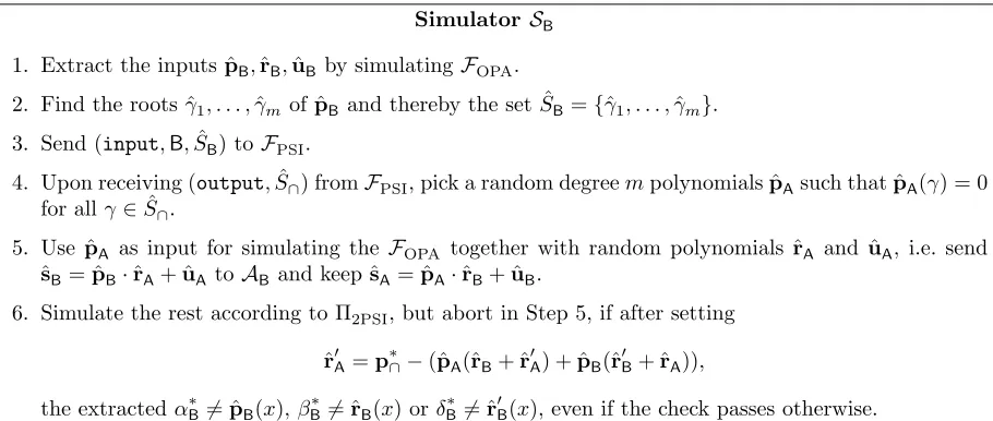
Corrupted Alice. We show the indistinguishability of the simulation ofSA(cf. Figure 10). The simulator extracts Alice’s inputs and then checks for any deviating behaviour. If such behaviour is detected, it aborts, even if the protocol would succeed. Proving indistinguishability of the simulation shows that the check in the protocol basically enforces semi-honest behaviour by Alice, up to input substitution.
Simulator SA
1. Extract the inputs ˆpA,ˆrA,uˆA by simulatingFOPA.
2. Find the roots ˆγ1, . . . ,ˆγmof ˆpA and thereby the set ˆSA={γˆ1, . . . ,γˆm}. 3. Send (input,A,SˆA) toFPSI.
4. Upon receiving (output,Sˆ∩) fromFPSI, pick a random degreempolynomial ˆpBsuch that ˆpB(γ) = 0
for allγ∈Sˆ∩.
5. Use ˆpB as input for simulating the FOPA together with random polynomials ˆrB and ˆuB, i.e. keep
ˆ
sB= ˆpB·ˆrA+ ˆuA and send ˆsA = ˆpA·ˆrB+ ˆuB to A.
6. Simulate the rest according to Π2PSI, but abort in Step 6, if after setting
ˆ
r0A = (s0∗A + ˆuA−uˆB−pˆAˆrB)/pˆA, α∗A6= ˆpA(x),β
∗
A6= ˆrA(x) orδ ∗ A 6= ˆr
0
A(x), even though the check would pass. Figure 10: Simulator SA against a corrupted Alice.
Consider the following series of hybrid games.
Hybrid 0: RealAA Π2PSI.
Hybrid 1: Identical to Hybrid 0, except that S1 simulates FOPA, learns all inputs and aborts if
α∗A 6= ˆpA(x) or βA∗ 6= ˆrA(x), but the check is passed.
Letα∗A =αA+ebe AA’s check value. Then the check in Step 6 will fail with overwhelming probability. Letσ denote the outcome of the check. IfAA behaves honestly, then
σ =α∗A(rB(x) +δ∗A) +pB(x)(β∗A+r0B(x))−p∩(x) = 0.
Usingα∗A =αA+e, however, we get
σ0 = (αA+e)(rB(x) +δA∗) +pB(x)(βA∗ +r0B(x))−p∩(x) =e·(rB(x) +δ ∗
A)6=const.
This means that the outcome of the check is uniformly random fromAA’s view over the choice ofrB (or pB forβ
∗
A 6=rA(x)). Therefore, the check will fail except with probability 2/|F|and Hybrids 0 and 1 are statistically close.
Hybrid 2: Identical to Hybrid 1, except thatS2 aborts according to Step 6 in Figure 10. An environment distinguishing Hybrids 1 and 2 must manage to send s0∗A such that
while passing the check in Step 6 with non-negligible probability.
Let f =s0∗A + ˆuA−uˆB−pˆA ·(ˆrB+ ˆr 0
A). We already know that f(x) = 0, otherwise we have
α∗A =αA+f(x)6=αA (or an invalidβ∗A), and the check fails. But sincexis uniformly random, the case that f(x) = 0 happens only with probability m/|F|, which is negligible. Therefore, Hybrid 1 and Hybrid 2 are statistically close.
Hybrid 3: Identical to Hybrid 2, except thatS3 generates the inputs ˆsA,ˆsB according to Step 5
in Figure 10 and adjusts the output. This corresponds to IdealSA
FPSI.
The previous hybrids established that the inputs ˆpA,ˆrA are extracted correctly. Therefore, by
definition, ˆSA =M0(ˆpA). It remains to argue that the simulated outputs are
indistinguish-able. First, note that the received intersection ˆS∩ = M0(ˆpB) defines ˆpB. From Lemma 6
it follows that M0(p∩) = M0(ˆpA)∩ M0(ˆpB) = ˆS∩ w.r.t. M0(ˆpB), even for a maliciously
chosen ˆrA, i.e. theAA cannot increase the intersection even by a single element except with
negligible probability.
Further, note that ˆsA = ˆpA·ˆrB+ ˆuB is uniformly distributed over the choice of ˆuB, and ˆp∩ is uniform over the choice of ˆrB,ˆr0B.
Finally, since ˆrB,ˆr 0
B are uniformly random and the degree of ˆpB is m, i.e. maxi|Si|+ 1, the
values ˆαB, ˆβB and ˆδB are uniformly distributed as well. In conclusion, the Hybrids 2 and 3 are statistically close.
As a result we get that for all environments Z,
RealAA
Π2PSI(Z)≈sIdeal
SA FPSI(Z).
Corrupted Bob. The simulator against a corrupted Bob in Figure 11 (and therefore the proof) is essentially the same as the one against a corrupted Alice, except for a different way to check his inputs.
Simulator SB
1. Extract the inputs ˆpB,ˆrB,uˆB by simulatingFOPA.
2. Find the roots ˆγ1, . . . ,ˆγmof ˆpB and thereby the set ˆSB={γˆ1, . . . ,γˆm}. 3. Send (input,B,SˆB) toFPSI.
4. Upon receiving (output,Sˆ∩) fromFPSI, pick a random degreempolynomials ˆpAsuch that ˆpA(γ) = 0
for allγ∈Sˆ∩.
5. Use ˆpA as input for simulating the FOPA together with random polynomials ˆrA and ˆuA, i.e. send
ˆ
sB= ˆpB·ˆrA+ ˆuA toAB and keep ˆsA= ˆpA·ˆrB+ ˆuB.
6. Simulate the rest according to Π2PSI, but abort in Step 5, if after setting
ˆ
r0A=p∗∩−(ˆpA(ˆrB+ ˆr0A) + ˆpB(ˆr0B+ ˆrA)), the extractedα∗B 6= ˆpB(x),β
∗
B6= ˆrB(x) orδ ∗ B 6= ˆr
0
B(x), even if the check passes otherwise. Figure 11: Simulator SB against a corrupted Bob.
Hybrid 0: RealAB Π2PSI.
Hybrid 1: Identical to Hybrid 0, except that S1 simulates FOPA, learns all inputs and aborts if
α∗A 6= ˆpA(x) or βA∗ 6= ˆrA(x), but the check is passed.
This step is identical to the case of a corrupted Alice. Let α∗B =αB+ebeAB’s check value. Then the check in Step 5 will fail with overwhelming probability. Letσ denote the outcome of the check. If AB behaves honestly, then
σ =α∗B(rA(x) +δ ∗
B) +pA(x)(β ∗ B+r
0
A(x))−p∩(x).
Usingα∗B =αB+e, however, we get
σ0 = (αB+e)(rA(x) +δB∗) +pA(x)(βB∗ +r0A(x))−p∩(x) =e·(rA(x) +δ ∗
B)6=const.
This means that the outcome of the check is uniformly random fromAB’s view over the choice ofrA (or pA forβB∗ =6 rB(x)). Therefore, the check will fail except with probability 2/|F|and Hybrids 0 and 1 are statistically close.
Hybrid 2: Identical to Hybrid 1, except thatS2 aborts according to Step 6 in Figure 11. An environment distinguishing Hybrids 1 and 2 must manage to send p∗∩ such that
p∗∩6= ˆpA(ˆrB+ ˆr 0
A) + ˆpB(ˆr 0
B+ ˆrA),
while passing the check in Step 5 with non-negligible probability.
Letf =p∗∩−(ˆpA(ˆrB+ ˆr 0
A) + ˆpB(ˆr 0
B+ ˆrA)). We already know thatf(x) = 0, otherwise we have
α∗B =αB+f(x)6=αB (or an invalidβ∗B), and the check fails. But sincexis uniformly random, the case that f(x) = 0 happens only with probability m/|F|, which is negligible. Therefore, Hybrid 1 and Hybrid 2 are statistically close.
Hybrid 3: Identical to Hybrid 2, except thatS3 generates the inputs ˆsB,ˆsA according to Step 5
in Figure 11 and adjusts the output. This corresponds to IdealSB
FPSI.
The previous hybrids established that the inputs ˆpB,ˆrB are extracted correctly. Therefore, by definition, ˆSB =M0(ˆpB). It remains to argue that the simulated outputs are
indistinguish-able. First, note that the received intersection ˆS∩ =M0(ˆpA) defines ˆpA. From Lemma 6 it
follows thatM0(p∩) =M0(ˆpB)∩ M0(ˆpA) = ˆS∩ w.r.t.M0(ˆpA), even for a maliciously chosen
ˆ
rB, i.e. AB cannot increase the intersection even by a single element except with negligible probability.
Further, note that ˆsB = ˆpB·ˆrA+ ˆuA is uniformly distributed over the choice of ˆuA, and ˆp∩ is uniform over the choice of ˆrA.
Finally, since ˆrA,ˆr0A are uniformly random and the degree of ˆpA is m, i.e. maxi|Si|+ 1, the values ˆαA, ˆβA and ˆδA are uniformly distributed as well. In conclusion, the Hybrids 2 and 3
are statistically close.
As a result we get that for all environments Z,
RealAB
Π2PSI(Z)≈sIdeal
Efficiency. The protocol makes two calls to OPA, which in turn is based on OLE. Overall, 2m calls to OLE are necessary in OPA. Given the recent constant overhead OLE of Ghosh et al. [GNN17], the communication complexity of Π2PSI lies inO(m).
On the computational side, the parties have to compute interpolations of polynomials of degree
m, which brings the computational complexity to O(mlogm) using NTT. Note that this cost includes the computational cost of the OLE instantiation from [GNN17]. This concludes the proof.
6
Maliciously Secure Multi-party PSI
6.1 Ideal Functionality
The ideal functionality for multi-party private set intersectionFMPSI* simply takes the inputs from all parties and computes the intersection of these inputs. Our functionality FMPSI* in Figure 12 additionally allows an adversary to learn the intersection and then possibly update the result to be only a subset of the original result.
FMPSI*
LetAdenote the set of malicious parties, andHthe set of honest parties.
1. Upon receiving a message (input, Pi, Si) from partyPi, store the setSi. Once all inputsi∈[n] are input, setS∩=Tn
i=1Si and send (output, S∩) toA.
2. Upon receiving a message (deliver, S∩0) from A, check if S∩0 ⊆ S∩. If not, set S∩0 = ⊥. Send
(output, S∩0) to H.
Figure 12: Ideal functionalityFMPSI* for multi-party PSI.
Let us briefly elaborate on why we chose to use this modified functionality. In the UC setting, in order to extract the inputs of all malicious parties, any honest party has to communicate with all malicious parties. In particular, since the simulator has to extract the complete input, this requires at leastO(nm) communication per party for the classical MPSI functionality. In turn, for the complete protocol, this means that the communication complexity lies inO(n2m).
and may not changed arbitrarily by the adversary. We believe that this weaker multiparty PSI functionality is sufficient for most scenarios.
6.2 Multi-party PSI from OLE
Our multi-party PSI protocol uses the same techniques that we previously employed to achieve two-party PSI. This is similar in spirit to the approach taken in [HV17], who employ techniques from the two-party PSI of [FNP04] and apply them in the multi-party setting. We also adopt the idea of a designated central party that performs a two-party PSI with the remaining parties, because this allows to delegate most of the computation to this party and saves communication. Apart from that, our techniques differ completely from [HV17]. Abstractly, they run the two-party PSI with each party and then use threshold encryption and zero-knowledge proofs to ensure the correctness of the computation. These tools inflict a significant communication and computation penalty.
In our protocol (cf. Figure 13) we run our two-party PSI between the central party and ev-ery other party, but we ensure privacy of the aggregation not via threshold encryption and zero-knowledge proofs, but instead by a simple masking of the intermediate values and a polynomial check. This masking is created in a setup phase, where every pair of parties exchanges a random seed that is used to create two random blinding polynomials which cancel out when added.
Once the central party receives all shares of the computation, it simply add these shares, thereby removing the random masks. The central party broadcasts the result to all parties. Then, all parties engage in a multi-party coin-toss and obtain a random value x. Since all operations in the protocol are linear operations on polynomials, the parties evaluate their input polynomials on x
and broadcast the result. This allows every party to locally verify the relation and as a consequence also the result. Here we have to ensure that a rushing adversary cannot cheat by waiting for all answers before providing its own answer. We solve this issue by simply committing to the values first, and the unveiling them in the next step. This leads to malleability problems, i.e. we have to use non-malleable commitments3.
Let us briefly give an intuition on why this protocol computes the intersection of all parties. The intersection polynomialp∩ =Pn
−1
i=1 (p0+pi)·(ri+r i
0) is the sum of all two-party intersection
polynomials. Every such intermediate polynomial contains exactly the intersection between the parties Pi and P0 in its roots (plus some additional, but random, roots). By simply adding all
of these polynomials, the common roots of the intermediate polynomials are preserved, while the other roots are blinded by random values. The probability that two of these random blindings cancel out is negligible in the field size. Therefore, from the view of each party, the common roots of p∩ and pi represent the intersection with all other parties.
Theorem 2. The protocol ΠMPSI computationally UC-realises FMPSI* in the FOPA-hybrid model with communication complexity in O((n2+nm)κ).
Proof. We have to distinguish between the case where the central party is malicious and the case where it is honest. We show UC-security of ΠMPSI by defining a simulatorS for each case which
produces an indistinguishable simulation of the protocol to any environmentZtrying to distinguish
3
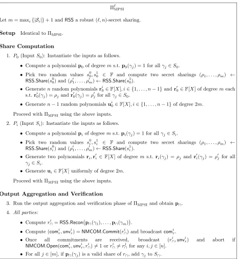
ΠMPSI
Letm= maxi{|Si|}+ 1 andNMCOMbe a bounded-concurrent non-malleable commitment scheme against synchronized adversaries. FOPA(i,j) denotes thejth instance for partiesP0andPi.
Setup
1. All partiesPiandPj fori, j∈ {1, . . . , n−1}exchange a random polynomial as follows. For allj6=i, ifvij =⊥,Pi picksseedij uniformly at random and setsvij =PRG2m(seedij). It sendsseedij toPj, who setsvji=−PRG2m(seedij).
Share Computation
2. P0 (Input S0): Compute a polynomial p0 of degree m s.t.p0(γj) = 0 for all γj ∈S0. Generate n
random polynomialsri0∈F[X], i∈ {1, . . . , n−1}andr 0
0∈F[X] of degreemeach andn−1 random
polynomialsui0∈F[X], i∈ {1, . . . , n−1} of degree 2m. Fori∈[n−1] • Inputri0,u
i
0 intoF (i,1)
OPA for eachi∈ {1, . . . , n−1}. • Inputp0into F
(i,2)
OPA and obtains
i
0=p0·ri+ui.
3. Pi (Input Si): Compute a polynomialpi of degree m s.t.pi(γj) = 0 for allγj ∈Si. Additionally, pickri,r
0
i∈F[X] uniformly of degreemandui∈F[X] uniformly of degree 2m. • Inputpi intoF
(i,1)
OPAand obtainsi=pi·r i
0+u
i
0.
• Inputri,ui into F
(i,2) OPA. • Sets0i=si−ui+pir
0
i+
P
i6=jvij and send it toP0.
Output Aggregation and Verification
4. P0: Computep∩=Pn−1
i=1 (s 0
i+s i
0−u
i
0+p0r 0
0) and broadcastp∩.
5. All parties:
• Run a multiparty coin-toss protocol ΠCT to obtain a randomx∈F.
• Evaluate αi = pi(x), βi = ri(x), δi = r
0
i(x) and compute (comi,unvi) = NMCOM.Commit(αi, βi, δi). Broadcastcomi.
• Once all commitments are received, broadcast unvi and (αi, βi, δi). Abort if
Pα
0·(βi+δ0) +αi·(β0+δi)6=p∩(x) orNMCOM.Open(comi,unvi,(αi, βi, δi))6= 1.
• For eachγj ∈Si: ifp∩(γj) = 0, addγj to S∩. OutputS∩.
Figure 13: Protocol ΠMPSI UC-realisesFMPSI* in the FOPA-hybrid model.
for the honest parties. We show that A can only reduce the intersection unless it already knows
x ∈Sj for at least one j ∈H, i.e. we assume that A cannot predict a single element of the set of an honest party except with negligible probability. This reduced intersection can be passed by the simulator to the ideal functionality.
P0 is malicious: Consider the simulator in Figure 14.
Simulator SP0
LetA={i|Pi is malicious}denote the index set of corrupted parties, where|A|=t≤n−1. Further letH denote the index set of honest parties.
1. Simulate the setup and obtain all v∗ij for i ∈A and j ∈H. Pick uniformly random ˆvjl ∈F[X] of
degree 2mforj, l∈Hand set ˆvlj=−ˆvjl.
2. Extract the inputs (ˆpj0,ˆrj0,uˆj0) ofP0 for allj∈Hby simulatingFOPA.
3. Abort in Step 5 of ΠMPSI if the ˆpj0 are not all identical. Set ˆpA= ˆpj0 for a randomj∈H, and find the roots ˆγ1, . . . ,γˆ2mof ˆpA and thereby the set ˆSA ={ˆγ1, . . . ,ˆγ2m}.
4. Send (input, Pi,SˆA) toFMPSI* for all partiesi∈A. 5. Upon receiving (output,Sˆ∩) fromF
*
MPSI, pick n−t random degree m polynomials ˆpj such that ˆ
pj(γ) = 0 for allγ∈Sˆ∩, j∈H.
6. Use the ˆpjas input for each instance ofFOPAtogether with random polynomials ˆrjand ˆujforj∈H, i.e. send ˆsj0= ˆpj0·ˆrj+ ˆuj toAand keep ˆsj = ˆpj·ˆr
j
0+ ˆu
j
0.
7. Simulate the rest according to ΠMPSI, but abort in Step 5, if the extracted ˆpA(x)6=α0or ˆr
j
0(x)6=β
j
0
for anyj∈H, even if the check passes otherwise.
8. Upon receivingp∗∩ fromA, if the check in Step 5 of ΠMPSIpasses, test for all s∈Sˆ∩ ifp∗∩(s) = 0.
If yes, set ˆS0∩= ˆS∩0 ∪s. Send (deliver,Sˆ∩0) toFMPSI* .
Figure 14: Simulator SP
0 forP0 ∈A.
We show the indistinguishability of the simulation and the real protocol through the following hybrid games. In the following, letA denote the dummy adversary controlled by Z.
Hybrid 0: RealAΠMPSI.
Hybrid 1: Identical to Hybrid 0, except thatS1 simulatesFOPA and learns all inputs.
Hybrid 2: Identical to Hybrid 1, except thatS2 aborts according to Step 7 in Figure 14.
Hybrid 3: Identical to Hybrid 2, except thatS3 aborts if the extracted ˆp0 are not identical, but the check is passed.
Hybrid 4: Identical to Hybrid 3, except that S4 replaces the vjl between honest parties j, l by uniformly random polynomials.
Hybrid 5: Identical to Hybrid 4, except that S5 generates the inputs ˆsj0,ˆsj according to Step 6 in Figure 14 and adjusts the output. This corresponds to IdealSP0
FMPSI*