Implementation of blind source separation of speech signals using independent component analysis

Implementation of blind source separation of speech

signals using independent component analysis

Vivek Anand. Dr. R. S. Anand.Dr. M. L. Dewal

Department of Electrical Engineering,

Indian Institute of Technology Roorkee, Roorkee – 247 667, Uttarakhand, India.

Abstract- Blind source separation (BSS) is the separation

of sources without having prior information about the mixtures. This is a major problem in real time world whether we have to identify a particular person in the crowd or it be an area of biomedical signal extraction like Electroencephalogram (EEG). It is really very difficult to estimate a source out of the mixtures. If the brain is malfunctioning, just by looking at the EEG we can’t say which part of brain is causing malfunction because the outputs are the mixtures from 21 electrodes. Similarly in a multiple speaker environment, when numbers of people are speaking simultaneously it is difficult to identify a particular speaker. Hence there is a need of source separation. Several methods are available for separating the sources like independent component analysis (ICA), auto decorrelation filtering (ADF) and beamforming. Here ICA has been used for the purposes of separation of signals and Matlab –GUI has been implemented for creating the user friendly environment.

Key Words: Blind source separation, Independent component analysis, Mixing signals, Unmixing signals

1. INTRODUCTION

BSS is a well researched area. One key advantage of ICA is that the microphone location and speaker locations do not need to be known in advance. Consequently the restriction on sensor placement is less critical as compare to the beam-forming techniques.Independent component analysis (ICA) is a well-known method of finding latent structure in data. ICA is a statistical method that expresses a set of multidimensional observations as a combination of unknown latent variables. These underlying latent variables are called sources or independent components and they are assumed to be statistically independent of each other. The ICA model is

x



f

(



,

s

)

Where

x



(

x

1

,

x

2

...

....

x

m

)

is an observed vector and

f

is a general unknown function with parameters



that operates on statistically independent latent variables listed in the vector

s



(

s

1

,

s

2

...

..

s

n

)

When the function is linear, and we can write

X



AS

Where

A

is an unknown mixing matrix. We consider

x

and

s

as random vectors. When a sample of observations

)

....

...

,

(

x

1

x

2

x

m

x



becomes available, we write

AS

X



where the matrix

X

has observations

x

as its columns and similarly the matrix

S

has latent variable vectors

s

as its columns. The mixing matrix

A

is constant for all observations. If both the original sources

S

and the way the sources were mixed are all unknown, and only mixed signals or mixtures

X

can be measured and observed, then the estimation of

A

and

S

is known as blind source separation (BSS) problem.

1.1 STATISTICAL INDEPENDENCE

Statistical independence is the key foundation of independent component analysis. For the case of two different random variables

x

and

y

,

x

is independent of the value of

y

if knowing the value of

y

does not give any information on the value of

x

. Statistical independence is defined mathematically in terms of the probability densities as: the random variables and are said to be independent if and only if

)

(

)

(

)

,

(

X

Y

P

X

P

Y

P

_xy



_{x y}

Where

P

xy

(

X

,

Y

)

is the joint density of

x

and

y

,

)

(

X

P

x

P

y

(

Y

)

and are marginal probability densities of

x

and

y

respectively. Marginal probability density function of

x is defined as

dy

Y

X

P

X

P

_x

(

)





_x,y

(

,

)

Other way stated, the density of

s

₁ is unaffected by

s

₂, when two variables

s

₁ and

s

₂ are independent. Statistical independence is a much stronger property than uncorrelated behaviour which takes into account the second order statistics only. If the variables are independent, they are uncorrelated but the converse is not true [1].

1.2 CENTRAL LIMIT THEOREM







k i i K

Z

X

1

be a partial sum of sequence

Z

_i of independent and identically distributed random variables

Z

_i. Since the mean and variance of

X

_k can grow without bound as, consider the standardized variables

Y

_k instead of

X

_k,

K K X X K K

m

X

Y







Where

m

and



are mean and variance of

X

_k .The distribution of

Y

_k converges to a Gaussian distribution with zero mean and unit variance when

K





This theorem has a very crucial role in ICA and BSS. A typical mixture or component of the data vector

x

is of the form







N j j ij i

a

S

X

1

Where

a

,

j



1

,

2

,

3

...

.

N

are constant mixing coefficients and

s

,

j



1

,

2

,

3

...

.

N

are the

N

unknown source signals. The central limit theorem can be stated as “the sum of even two independent identically distributed random variables is more Gaussian than the original random variables” [2]. This implies that independent random variables are more non-Gaussian than their mixtures. Hence non-Gaussianity is independence.

1.3 CONTRAST FUNCTIONS FOR ICA

The data model for independent component analysis is estimated by formulating an objective function and then minimizing or maximizing it. Such a function is often called a contrast function or cost function or objective function. The optimization of the contrast function enables the estimation of the independent components. The ICA method combines the choice of an objective function and an optimization algorithm [3]. The statistical properties like consistency, asymptotic variance, and robustness of the ICA technique depend on the choice of the objective function and the algorithmic properties like convergence speed, memory requirements, and numerical stability depend on the optimization algorithm. The contrast function in some way or other is a measure of independence. In this section different measures of independence is discussed which is frequently used as contrast functions for ICA.

1.4 MEASURING NON GAUSSIANITY Kurtosis:

According to the Central limit theorem, non -Gaussianity is a strong measure of independence. Traditional higher order statistics uses kurtosis or the named fourth-order cumulant to measure non-Gaussianity. The kurtosis of a zero-mean random variable v is defined by

2 2 4

})

{

(

3

}

{

)

(

v

E

v

E

v

Kurt





Where

E

{

v

4

}



Fourth moment of

v

E

{

v

2

}



Second moment of

v

For a Gaussian random variable

v

, the

E

{

v

4

}

equal

,

})

{

(

3

E

v

2 2 so that the kurtosis is zero for a Gaussian random variable. If v is a non-Gaussian random variable, its kurtosis is either positive or negative. Particularly when kurtosis value is positive the random variables are called

Supergaussian or Leptokurtic and when negative called

Subgaussian or Platykurtic. Supergaussian random variables have a spiky probability density function with heavy tails and subgaussian random variables have a flat probability density function. Thereore, non-gaussianity is measured by the absolute value of kurtosis [4].

1.5 DATA PRE-PROCESSING FOR ICA

It is often beneficial to reduce the dimensionality of the data before performing ICA. It might be well that there are only a few latent components in the high-dimensional observed data, and the structure of the data can be presented in a compressed format. Estimating ICA in the original, high-dimensional space may lead to poor results. For example, several of the original dimensions may contain only noise [5]. Also, over learning is likely to take place in ICA if the number of the model parameters (i.e., the size of the mixing matrix) is large compared to the number of observed data points. Care must be taken, though, so that only the redundant dimensions are removed and the structure of the data is not flattened as the data are projected to a lower dimensional space. In this section two methods of dimensionality reduction are discussed: principal component analysis and random projection.

In addition to dimensionality reduction, another often used pre processing step in ICA is to make the observed signals zero mean and décorrelate them. The decorrelation removes the second-order dependencies between the observed signals. It is often accomplished by principal component analysis which will be briefly described next.

1.6 PRINCIPAL COMPONENT ANALYSIS

In principal component analysis (PCA), an observed vector

x

is first centred by removing its mean (in practice, the mean is estimated as the average value of the vector in a sample). Then the vector is transformed by a linear transformation into a new vector, possibly of lower dimension, whose elements are uncorrelated with each other. The linear transformation is found by computing the Eigen value decomposition of the covariance matrix. For a zero-mean vector

x

, with

n

elements, the covariance matrix

C

_X is given by: T

T

X

E

XX

EDE

C



{

}



Where

E



(

e

1

,

e

2

...

e

n

)

=Orthogonal matrix of

)

...

,

(

1 2 n

diag

D











Diagonal matrix of Eigen

value of

C

_X

Whitening or Sphering can be described as

X

P

Z



*

Where

P

is the whitening matrix and

Z

is a new matrix that is white.

P

is defined as T

E

D

P



0.5



Subsequent ICA estimation is done on

Z

instead of

X

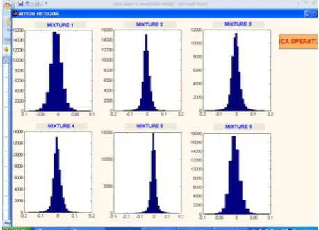
. For whitened data it is enough to find an orthogonal demixing matrix if the independent components are also assumed white. Dimensionality reduction can also be accomplished by methods other than PCA. These methods include local PCA and random projection [6][7].

During Experiments we recorded the 6 voice samples from each of 25 speakers. Out of the total of 150 samples we have taken various combinations of 6 samples in such a manner so that each sample belongs to a different speaker. We have made 6 linear mixtures for each of these combinations using matlab coding. FASTICA algorithm has been applied on each of these set of mixtures. These mixtures have been separated out into corresponding independent components. In order to check the accuracy of algorithm, we have plotted histograms corresponding to sources, linear mixtures and independent components. We have found peaky histograms for speech sources, Gaussian histograms for mixtures and non-Gaussian histograms for independent components. Results are observed by listening to the output voice signals through headphone which are shown in figure 5. The resultant voice signals are very clear.

This paper is organized as follows. Section 2 summarizes the Fast ICA algorithm, which is used for the separation purposes. Details of database, which is used during experiments, are given in section 3. Results and discussions are given section 4.

2. FAST ICA ALGORITHM

The Fast ICA algorithm involves the following steps. 1. Make the available mixed data zero mean. 2. Whiten the data.

3. Choose an initial weight vector w of unit norm.

w

w

w

_norm



4. Let

w

m

w

g

m

E

m

w

g

m

E

w

_new



{

_i

(

T _i

)}



{

_i

'

(

T _i

)}

This is the basic weight update equation, where g is the contrast function. 5. Let new new new

_w

w

w



This is the normalization step that makes the new w as unit norm, which will be updated at every iteration. Compare

new

w

with the old vector, if converged than move ahead, if not go to step 4[8] [9].

3. DETAILS OF DATABASE

For Experimentation purposes we have recorded the database. The Details of database are as follows.

Total number of speakers: 25 Number of audio files per speaker: 6 Total number of audio files recorded: 150 Number of male speakers: 23

Number of female speakers: 02 Duration of recording: 5 seconds

Size of each audio file: 500 kb with double class format. Sampling frequency: 12500 samples per second Number of samples per speaker: 62500

Speech samples consist: newspaper reading, songs, mantras, introduction of speakers.

Languages used: Hindi, English, Punjabi, Bengali, Tamil, Telgu, Gujarti, Marathi, Malayalam.

4. RESULTS AND DISCUSSION

We have successfully implemented Mat lab-GUI for the separation of speech mixtures using FAST ICA algorithm. We have found very good results of all performed experiments. Play buttons have been incorporated in GUI window by which we can listen source signals, mixtures and independent components in the corresponding window. Sampling frequency should be the same for source signals, mixtures as well as independent components otherwise quality separation will not be achieved.

When the mixtures are nonlinear convolutive mixtures and reverberation of room environment is high then conventional ICA does not perform well because of an unknown transfer function of the room will be generated due to impulse response of acoustic impedance. This impedance will be there because of the walls, wood and glasses. Hence algorithm can be developed to implement ICA in frequency domain for nonlinear convolutive mixtures.

5. CONCLUSIONS

We were reliably able to record independent speech signals, digitally mix them to create linear speech mixtures, and then recover the independent components using ICA. Blind source separations of 6 speech signals using the ICA algorithm have done.

Figure 1 Representing six speech source signals.

Figure 2 Representing peaky histograms corresponding to source signals.

Figure 3 Representing linear mixtures of sources.

Figure 4 Representing Gaussian histograms of corresponding mixtures.

Figure 5 Representing six independent components extracted from mixtures through ICA.

REFERENCES

[1] Z.Koldovsky and P.Tichavsky “Time-Domain Blind Audio

Source Separation using Advanced ICA Methods”. Proc. INTERSPEECH 2007 ,Antwerp, Belgium , august 2007

[2] Apo Hyvarinen and Erkki Oja, ”Independent Component

Analysis: Algorithms and Applications . Neural Networks Research Centre, Helsinki University of Technology,http://www.csi.hut.fi/Projects/ica,2000.

[3] Taesu Kim,Attias,H.T.,Soo-Young Lee and Te-Won Lee,”Blind

Source Separation Exploring Higher-Order Frequency dependencies”,IEEE Transactions on Speech and Audio Processing,Vol 15,No1,Jan 2007,pp 70-79.

[4] A. Belouchrani, K. Abed-Meraim, J. Cardoso, and E. Moulines,

“A blind source separation technique using second-order statistics,” IEEE Trans. Signal Process. 45, 434–444 (1997)

[5] Y. Zhao, R. Hu and X. Li,”Speedup Convergence and Reduce

Noise for Enhanced Speech Separation and Recognition”IEEE Trans.Audio, Speech and Language Processing, Vol.14, no.4.July 2006.

[6] N.Murata, S.Ikeda, and.Ziehe, BSIS Technical Report, 98-2

Apr.1998.

[7] Hyvarinen, A., "Fast and robust fixed-point algorithms for

independent component analysis", Neural Networks, IEEE

Transactions on, On page(s): 626 - 634, Volume: 10 Issue: 3, May 1999

[8] Hyvarinen, A., "Gaussian moments for noisy independent

component analysis", Signal Processing Letters, IEEE, On

page(s): 145 - 147, Volume: 6 Issue: 6, Jun 1999

[9] S. Amari, A. Cichocki, and H. H. Yang, "A new learning