ISSN 2286-4822 www.euacademic.org
Vol. II, Issue 6/ September 2014
Impact Factor: 3.1 (UIF) DRJI Value: 5.9 (B+)
Build Mathematical Model by MANET
Parameters
ZEINA H. AL- HADAD
Department of Computer Science Kufa University Iraq
Abstract:
A mathematical model was built and implemented to estimate the optimal number of nodes required to be deployed in each new designed MANETs environment. Many queuing theory parameters were used to study and analyze the behavior of the MANETs.
Mobile Ad-hoc Network (MANET) was defined as a set of mobile nodes that moved freely and connected among each other without any infrastructure or administrator control. Each node contains a kind of queuing system like buffer used it to serve the arriving packets that reached to the busy node. The packets reach each node in certain sequence. The number of received (arriving packets) per unit time is called “arrival rate". The average rate or the average time between any two successive packets is called the inter- arrival time and follow certain statistical distributions. The node will serve the packets according to certain mechanism (discipline) like drop tail.
Key words: MANET, NS-2, DropTail, Mobility Model, Queuing,
DSDV, Mathematical model.
Introduction
infrastructure or centralized administration. MANET capabilities and its applications are expected to become an important part of overall next-generation wireless network functionalities. MANET's nodes are free to move randomly. Such network’s topology may change rapidly and unpredictably. Each mobile node can have one or more network interface, each of which is attached to a channel . Channels are the conduits that carry packets between mobile nodes. When a mobile node transmit a packet to a channel, the channel distributes a copy of the packet to all the other network interface on the channel. These interface then use a radio propagation model to determine if they are actually able to receive the packet [ D. B. Johnson, et al., 1999].
Queuing theory is the process of handling the sequence of activities that arrives to certain server in certain shape. The server will serve these arriving units in certain order. In MANETs the nodes will serve the arriving packets in certain discipline (FIFO (Drop Tail), PRIORITY, RED, etc). The effects of the sent packets mean inter arrival time and packets mean service times on the network nodes idle times, loss packets, mean servers (nodes) utilization and throughput were studied and analyzed in this study [Moshe Zukerman].
Queuing Concept
leaves the network. Customers that complete their service in one queuing system goes to another and then to another and so forth, and never leaves the network. In open queuing systems new customers from outside of the network can join any queue, and when they complete their service in the network obtaining service from an arbitrary number of queuing system they may
leave the network [Moshe Zukerman].
Performance Evaluation
Many performance metrics were developed to collect and report the required information to measure the performance of the networks. All of the measuring performance processes requires the use of statistical modeling to determine the results [Odge, 2003]. This study deals with the following important performance metrics.
1- Throughput
It is represents the mount of data received by the destination nodes through period of time [Ravi Kumar Bansal, 2006].
Throughput=receive packets/simulation time
2- Dropped Packets
It is the number of packets that sent by the source node and fail to reach to the destination node [Aliff Umair Salleh, et al., 2006].
Dropped packets = sent packets(i) – received packets(i)
3- Mean Inter Arrival Time
The arrival process is characterized by the arrival time ari of
the packets or customers (received packets) and it can be computed by the following equation:
ai= (ar i –ar (i-1)
Mean arrival time average is the summation of inter-arrival times by the number of received packets (n) :
4- System Busy Time
system Busy time represents the total service times of the server [Hyungwook Park, 2009].
B = ∑ si
5- System Idle Time
If the queue is empty and the server is idle, a new packet is immediately sent to the node for service, otherwise the packet remains in the queue joining the waiting line until the queue is empty and the server becomes idle. The system idle time (I) can be computed by the following equation [Hyungwook Park, 2009].
I = T- B .
Where T is the simulation time and B is the busy time.
6- Mean Server Utilization
The server utilization is one of the important indication to design systems that will maintain high utilization [Moshe Zukerman]. Mean server utilization is the percentage of time where the server is busy. The server utilization (U) can be estimated by the following equation.
U = B/ T
7- Mean Service Time
Mean service time (S) is the average required time for each packet to be served (or to be forwarded for certain cases). It can be computed by the following equation :
S=∑si /n
where si is the service time of ith packets and n is the number
of the sent packets.
Simulation Environment
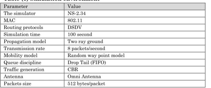
Table (1) Simulation environment
Parameter Value
The simulator NS-2.34
MAC 802.11
Routing protocols DSDV Simulation time 100 second Propagation model Two ray ground Transmission rate 8 packets/second Mobility model Random way point model Queue discipline Drop Tail (FIFO) Traffic generation CBR
Antenna Omni Antenna
Packets size 512 bytes/packet
To evaluate the performance metrics with different MANET's parameters such as varying numbers of nodes and different areas. Table (2) shows these MANET's variables values.
Table (2) The suggested MANET variables. Case
number Nodes number Speed
Pause time
Simulation area
1 3,4,5,6,7,8 10m/s 6s 500m*500m
2 4,5,6,7,8,9,10,11,12,13 10m/s 6s 800m*800m
3 6,7,8,9,10,11,12,13,14,15,16,17,18 10m/s 6s 1000*1000
Simulation Results
In order to collect the required data and information to be used in queuing modeling, the following steps were proposed to be followed during the implementation of the NS-2 to simulate the suggested designed MANET scenarios in this paper.
Step1: start.
Step2: build the traffic generators between the mobile nodes using the "cbrgen".
Step3: generate the movement file (scenario file) for the suggested MANET using the "setdest".
Step5: feed this "tcl" file with the traffic file and the scenario file to achieve the simulation process. At this step, two files (trace file and NAM file) are resulted. Step6: compute the average values for each metric. Step7: apply the mathematical model based on the average values for certain metrics (selected maximum value) which indicate the best nodes number for this MANET.
Step8: end.
Probability Computations
The authors were tried to compute the probability of finding receiving packets of destination node during the simulation time with different areas using the following developed equation :
; av is the average execution of the 25 runs
and Ts is the run simulation time.
The similar equation was also used to compute the probability of the lost packets, busy time, idle time and mean server utilization during the simulation time. The following figures show these probabilities for certain performance metrics.
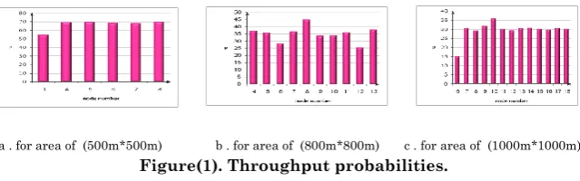
Figure (1) clarifies the probability of the throughput during simulation time within different with different areas.
a . for area of (500m*500m) b . for area of (800m*800m) c . for area of (1000m*1000m) Figure(1). Throughput probabilities.
a . for area of (500m*500m) b. for area of (800m*800m) c. for area of (1000m*1000m) Figure(2). Probability of the lost packets.
Histograms in figure (3) show the probability of the busy time, idle and utilization for varying number of nodes with area
500*500m.
a . probability of busy time. b . probability of idle time. c . probabilityof mean server utilization Figure (3). The probability of busy, idle and utilization with area of (500m*500m).
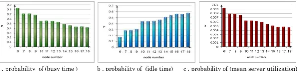
Histograms in figures (4) and figure(5) shows the probability of busy ,idle and utilization for varying number of nodes with area of 800m*800 m and area of 1000m*1000m respectively.
a . probability of (busy time ) b . probability of (idle time) c . probability of (mean server utilization) Figure(4) . The probability of busy ,idle and utilization with area of (800m*800m).
a . probability of (busy time ) b . probability of (idle time) c . probability of (mean server utilization)
In this study the Poisson equation was suggested to compute the packets arrival rate as a probability density function within each area :
!
)
/
1
(
)
(
/ 1
x
e
x
p
x
Where λ is average of inter arrival time and x node numbers in above table.
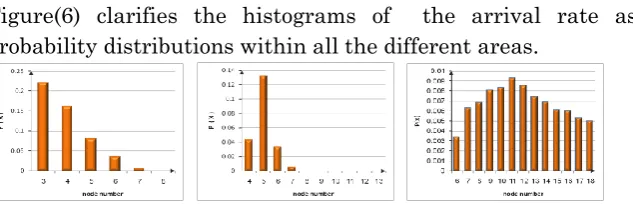
Figure(6) clarifies the histograms of the arrival rate as probability distributions within all the different areas.
Figure (6). Mean inter-arrival times for different number of nodes.
The Poisson equation was also used in calculating the service time as probability density function for each number of nodes with different areas :
Where µ is the mean service time and x is the number of nodes.
a . probability with (500m*500m) b. probability with (800m*800m) c . probability with ( 1000m*1000m) Figure(7). Probability of mean service time for varying number of nodes.
Mathematical Model
optimum number of nodes with certain area. So, this model gives more accurate information using the defined value probabilistic mathematical model. After experimentation with several equation on the calculated result tables.
The following equation was suggested and applied to calculate the value which indicate the best number of nodes in each area size.
V = ( AV_T(i) + (AV_U(i) *1000) - AV_L(i) - AV_I(i) )* e (µ+λ)
Where AV_T , AV_U, AV_L and AV_I are average of throughput, utilization, loss packets and idle time respectively. λ is the transmission rate( reception rate) and μ is the service rate.
This equation was applied and it is results were shown in tables (3) .These tables are clarifies the optimum number of nodes.
Tables (3) Results value and number of nodes with different areas.
Number
of node V
3 7735.174
4 10518.36
5 10893.28
6 10830.61
7 10813.63
8 10910.03
(a)
Area of 500m*500m
Number of node V
4 4496.434
5 4605.419
6 4781.228
7 6416.608
8 9207.82
9 6938.394
10 5647.1
11 5532.143
12 3975.586
13 3958.918
(b)
Area of 800m*800m
Number of node V
6 2033.63
7 6122.605
8 6145.126
9 7541.964
10 8977.607
11 7479.679
12 7383.792
13 7218.31
14 6126.22
15 6083.126
16 6039.263
17 5650.2
18 5516.251
(c) Area
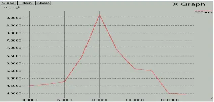
Figures (8), (9) and (10) shows graphs to indicate the maximum value which indicate the optimum number of nodes for different areas. X graph tool that supported by NS-2 was used to draw the results in the following figures.
Figure (8). Optimum value of nodes number for area of 500*500m.
In figure (8) shows that for area 500m*500m with DSDV protocol, the optimum number of nodes for this MANET is ( 5). This value represents the maximum value in the curve.
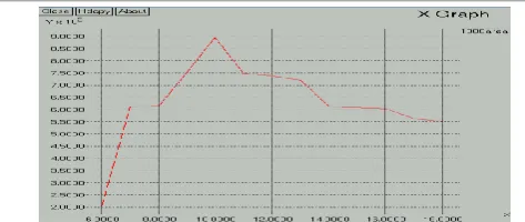
Figure(9). Optimum number of nodes for the area of 800*800m.
Figure (10). Optimum number of nodes for the area of 1000*1000m.
Figure (10) show that (10) nodes are optimal value for area 1000*1000 with routing protocol DSDV.
Conclusion
There are many tools that can be utilized to improve and develop the behavior of the MANETs. The well- known performance metrics were studied in the current and previous times by many researchers. This study concludes that there is a possibility to make use of many other performance metrics in addition to these well known metrics. These new metrics (or special used) were mixed with the other metrics to develop and estimate certain indications about the MANET's behavior.
A suggested mathematical model was built and
implemented to compute the optimal number of nodes for each MANET's area with the use of the DSDV routing protocol. The optimum number of nodes are depending on the effects of the mean inter arrival time, mean service time, maximum throughput, mean service utilization, minimum idle time and lost packets. Ns-2 was used as a simulation tool in simulating each of developed scenarios. The AWK language was also used to estimate many performance metrics values.
REFERENCES
Science and Engineering Department, Thapar Institute of Engineering and Technology, Deemend University, 2006.
Hyungwook, Park, "Parallel Discrete Event Simulation of Queuing Networks Using GPU-Based Hardware Acceleration", of the Requirements for The Degree of Doctor of Philosophy University of Florida , 2009.
Johnson, D. B., Josh Broch, Yih-Chun Hu, Jorjeta Jetcheva and David A.Maltz, "The CMU Monarch Project 's Wireless and Mobility Extensions to ns", computer science department Carnegie mellon university Pittsburgh, 1999
avilable [Online] : http://www.monarch.cs.cmu.edu/.
Odge, "The Oxford Dictionary of Statistical Terms", OUP.
ISBN0-19-920613-9, 2003,[Online].Available:
http://www.bth.se/fou/cuppsats.nsf/all.
Salleh, Aliff Umair, Zulkifli Ishak , Norashidah Md. Din and Md Zaini Jamaludin, "Trace Analyzer for NS-2", IEEE, pp. 29-32, Student Conference on Research and Development (SCOReD), Malaysia, 2006.
Zukerman, Moshe. Introduction to Queueing Theory and Stochastic Teletraffic Model, Teaching Textbook
Manuscript, Retrieved from