Using Michell Truss Principles to find an Optimal Structure Suitable for Additive Manufacturing

(1)

ABSTRACT

KRISHNAN, ARVIND SIVARAMA. Using Michell Truss Principles to find an Optimal Structure Suitable for Additive Manufacturing. (under the direction of Dr. John

Strenkowski.)

Additive Manufacturing (AM) technology is improving its capabilities in terms of

precision, variety of materials available, build time and mechanical properties of the final

part. Due to the nature of the process, the time required to manufacture a design is only

dependent on its dimensions and independent of the complexity of the geometry. It is now

used for rapid manufacturing in aerospace and biomedical applications and other industries

as well. Michell truss inspired optimum designs, which are complex to manufacture through

traditional methods, can now be made using AM technology. In this thesis, a new method for

finding the internal lattice of a Michell truss is introduced using a finite element analysis. For

a simply-supported beam, the internal shape is defined and an algorithm is used to optimize

the geometry taking AM constraints into account and the results are compared with existing

published data. Once the method is validated, the same procedure is applied to a cantilever

beam with a point end load. The internal lattice is defined and an optimization algorithm is

used to find the minimum required thickness of all struts to achieve a minimum weight beam.

(2)

(3)

Using Michell Truss Principles to find an Optimal Truss Structure Suitable for Additive Manufacturing

by

Arvind Sivarama Krishnan

A thesis submitted to the Graduate Faculty of North Carolina State University

in partial fulfillment of the requirements for the degree of

Master of Science

Mechanical Engineering

Raleigh, North Carolina

2015

APPROVED BY:

_______________________________ ______________________________

Dr. Scott Ferguson Dr. Kara Peters

________________________________ Dr. John Strenkowski

(4)

BIOGRAPHY

Arvind Krishnan was born in Doha, Qatar on February 28th, 1989 and grew up in

Mumbai, India. In 2005, his family moved to Austin, Texas where he studied at West Lake

High School. He completed his Bachelors of Science in Mechanical Engineering with high

honors from the University of Texas at Arlington. Then, he worked at GoEngineer as a

Simulation Technical Support Engineer for a couple of years.

Following this, Arvind moved to Raleigh, North Carolina to pursue his graduate

studies at the North Carolina State University beginning August 2013. During the summer of

2014, he interned at The Gigtank in Chattanooga, TN. Working as an Additive

Manufacturing Specialist, Arvind worked on multiple projects in collaboration with multiple

3D-Printing start-up companies.

Arvind enjoys playing Tennis, Badminton, Racquetball, Chess and Soccer. He is also

(5)

ACKNOWLEDGEMENTS

I would like to thank Dr. John Strenkowski for giving me the opportunity to work

under his guidance during my research. You have been open to new ideas and always had the

bigger picture in mind. Thank you Dr. Peters and Dr. Ferguson for being part of my

committee and providing valuable inputs.

I would not be here today without my amazing parents. Amma, you have sacrificed so

much and constantly catered to my unending needs. Appa, you have been my best friend,

mentor and protector at all times. My brother Anand has always been there to cover up when

I got into trouble with my continuous mischief. With you all by my side, no challenge seems

daunting, no task impossible and no mountain is too tall to climb. To my family, including

Kirti, thank you for the constant support.

My mentors Dr. Hyejin Moon, Dr. Kamesh Subbarao, Srinivas Krishnan, and Brad

Hansen, thank you for your continuous guidance during pivotal moments in my career.

To my undergraduate friends: Channa, Abhilash, Isura, Sunny, and Andie, here is to

all the crazy and irreplaceable memories, to the countless arguments about religion and

politics, plans to take over big companies, endless parties and family-like support. Thank you

all.

Graduate school has been a crazy ride thanks to the awesome people of Chai Khaana

Vagera (Tea, Snacks etcetera). The memories of coming home after a long day of work to tea

(6)

memory. A special note of appreciation to Subramaniam Iyer and Navneet Arakony, for

always caring and being there at all times.

Last, but not least, I’d like to mention Nikhil Shrivatsan, Ketan Shende, Shengqi

Zhang and Rohit Pagedar for helping me with the optimization algorithm, Arunachalam

Thiravium for valuable inputs on Michel truss layouts, and my optimization project group.

(7)

LIST OF TABLES

(11)

LIST OF FIGURES

Figure 1.1: Custom Chair Design……… …..1

Figure 2.1: Cube 3 Printer from 3D Systems……….4

Figure 3.1: Michell Truss Layout……… ………10

Figure 3.2: Alpha and Beta lines………..11

Figure 3.3: Stress Field for Perfectly Plastic Material……… ……….12

Figure 4.1: Discretized ESO Optimized Structure Shape……… ……16

Figure 4.2: Topology Optimization by Bubble Method………..17

Figure 5.1: Symmetrical Simply-Supported Beam...……… .……..23

Figure 5.2: Image of Symmetrical Simply-Supported Beam..……….……25

Figure 5.3: Stress-Strain Curve of Simply-Supported Beam………..……… ….26

Figure 5.4: Force-Deflection Curve for Simply-Supported Beam………..……….26

Figure 5.5: Simply-Supported Beam Model in ANSYS APDL……… …..27

Figure 5.6: Line Numbers for Reaction Force Comparison……….…………29

Figure 5.7: Deformed Shape of Simply-Supported Beam Model………... …….32

Figure 5.8: Maximum Stress in Simply-Supported Beam Model………. …...33

Figure 6.1: Principal Stress Trajectories for a Simply-Supported Beam……….35

Figure 6.2: FEA Model showing Constraints and Loads for Simply-Supported Beam ……..36

Figure 6.3: Original Michell Paper Example ……… ..37

Figure 6.4: Finite Element Model Setup for 2nd Model……… ..………37

Figure 6.5: Max and Min Principal Stress trajectories Superimposed on a CAD Model.. ..…39

Figure 6.6: Slip Lines Trajectories Superimposed for 2nd Model……… ………40

Figure 7.1: Flowchart for Simulated Annealing Algorithm……….………44

Figure 8.1: Hollow Model with Holes for Powder to Escape……….. ………50

Figure 8.2: Line Number for Simply-Supported Beam ANSYS Model.……….... 52

Figure 9.1: Fitness vs Iterations for Symmetrical Simply-Supported Beam………...55

Figure 9.2: CAD Model with Optimized Thicknesses……….………56

(12)

Figure 9.4: Maximum Stress Distribution for Optimized Design………. …...58

Figure 9.5: Minimum Stress Distribution for Optimized Design……….………59

Figure 9.6: Different Depths for Different Struts in Published Results………... ....60

Figure 9.7: Thicknesses of Struts Compared with Different Starting Thicknesses.…….……62

Figure 9.8: CAD Model of Optimized Beam……….……...……63

Figure 9.9: Deformation Results for Tetrahedral Mesh..……….…….…63

Figure 9.10: Additive Manufacturing Violations vs Iteration……….…….………65

Figure 10.1: Cantilever Beam Loading Conditions………..………68

Figure 10.2: Maximum and Minimum Principal Stress Trajectories………...69

Figure 10.3: Cantilever Beam Model Topology………..…….70

Figure 10.4: Michel Truss for Cantilever Beam with Point Load………....………71

Figure 10.5: FEA Setup for Point Load Cantilever Beam………. ….…….72

Figure 10.6: Line numbers for Additive Manufacturing Constraints………. ..…….…..73

Figure 10.7: Fitness vs Iteration……….…..75

Figure 10.8: Tensile Stress in Optimized Design……….…75

Figure 10.9: Compressive Stress in Optimized………76

Figure 10.10: Maximum Stress vs Iteration……….…77

Figure 10.11: Optimized CAD Model………..77

Figure 10.12: Deformation of Optimized Model………. …………78

(13)

1. INTRODUCTION

Over the past thirty years, three-dimensional (3D) printers have gained prominence as

an integral component in the design to manufacturing process. In this method, a CAD model

is additively manufactured one layer at a time using a 3D printer. Due to the nature of the

process, the time, cost and material required to manufacture a part is only dependent on its

dimensions and independent of the complexity of the geometry.

Originally, this technology was used mainly for prototyping purposes. However, with

improvements in various aspects of the technology like speed, material properties and cost of

production, there has been a gradual switch towards more end products and customized

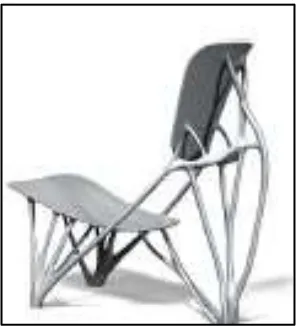
designs which allow this technology to be used by a more diverse range of people (1). One

such customized design of a chair can be seen in Figure 1.1 below (1).

Figure 1.1 Custom Chair Design

As expected, there are many engineering applications that can benefit from additive

(14)

the stiffest structure possible by using the least amount of material. Michell (3) laid the

foundations for such a structure by saying that all elements must follow paths of maximum

strain so that the topology is the stiffest for a given mass.

The resulting topology from such a structure is too complex for traditional

manufacturing techniques. However, with the use of additive manufacturing, it is now

possible to design such structures with no additional cost or time. In the past, design for

manufacturing guidelines would dictate that parts be kept simple so that manufacturing

process requirements such as draft angles and wall thickness could be adhered to. With this

new technology, parts can be made with greater complexity, and process considerations are

less prominent (4). There is a clear need for a methodology to optimize the creation of

complex shapes while taking the requirements of an additive manufacturing process into

consideration.

The objective of this thesis is to create a topology optimized design using a Michell

truss layout while also accounting for additive manufacturing constraints. The design

freedom provided by additive manufacturing (AM) will be utilized in designing a minimum

weight lattice structure. A brief background of the additive manufacturing industry, Michell

trusses, and optimization procedures is first described. The internal lattice of a

simply-supported beam is determined using a Michell truss as the basis of the structure. The mass of

the truss is minimized by optimizing the thickness of each strut in the truss and then it is

compared with an existing optimized design. The optimization algorithm used is called

(15)

A second example is provided of a Michell truss layout of a cantilever beam with a

point load. Although the additive manufacturing process affords new design freedom as

compared with more traditional manufacturing methods, it also requires that additional

constraints be satisfied. These constraints are described in the thesis and included in the

algorithm for manufacturing real parts. The algorithm and constraints described in this thesis

(16)

2. ADDITIVE MANUFACTURING INDUSTRY

2.1 Description and History

The industrial revolution paved the way to manufacture one part repetitively using

production lines. Men and woman operate highly automated machinery using a computer and

manufacturing facilities to produce parts (5). However, this approach is not cost effective if a

single part with a customized design is required. Manufacturers would need to invest in

tooling, casting and a unique suitable finishing technique. It would costs thousands of dollars

just to create one unique customized design (5). This is where additive manufacturing proves

useful.

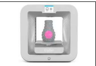
Figure 2.1 Cube 3 Printer from 3D Systems (6)

The 3D printing or additive manufacturing industry started with Chuck Hull who filed

a patent in 1986 for using Stereolithography to solidify a thin layer of liquid plastic and

(17)

3D printer manufacturer company, while other innovators used the concept of solidifying one

layer at a time to create new AM techniques and 3D printers. Figure 2.1 above shows a 3D

printer currently manufactured by 3D Systems.

The mechanical properties of the final part are dependent on which additive

manufacturing process is used and which options are selected for each of the parameters like

speed of printer head and temperature. These mechanical properties are constantly evolving

with time and research. The following sections briefly describe the different AM processes in

use today and some of the current on-going research.

2.2 Current Research and Industry Usage

In 2009, a meeting of 65 experts in the additive manufacturing field released a document titled ‘2009 Roadmap for Additive Manufacturing’. The document gave recommendations on

the direction of focus of research for the next few years in this field (7). Some recent research

developments are highlighted here. The parameters that determine the properties of the

finished part are:

 Purity of material used

 Mechanical properties of powder

 Printer head temperature relative to melting point of material

 Speed of the printer head, thickness of each layer, and

(18)

There has been considerable research to improve performance of these parameters.

Jariwala conducted a study on a process planning method with the ability to cure a film to

various thicknesses (8). Recently, greater emphasis has been focused on freedom of design to

manufacture parts, especially cellular structures, optimal designs and repeatable unit cells (9).

As additive manufacturing becomes a more integral part of how things are made, there is

research and development in supply chain management, and logistics for using additive

manufacturing (9). Microstructural lattice design is another area that is gaining prominence.

Recently, Krishnan Suresh developed a framework for the same, expecting increased

manufacturing through 3D printers in the near future (10). Using this, the density of the

lattice at different areas of a design can be altered based on the stress distribution, resulting in

weight reduction.

Although it is a new technology, many people own something that has been 3D

printed. This technology is also spreading to new markets. Customized foods of different

shapes and designs like pancakes and cakes are being 3D printed for special occasions.

Artists are using it to create 3D sculptures of varied complexity. Multiple start-ups and

research institutes like 3D Ops and Formlabs are trying to make replications of human organs

with 3D printers (11).

The aerospace industry manufactures complicated parts that must meet stringent

design requirements for strength and weight, but does not usually have high production

volumes. As a consequence, the aerospace industry has adopted AM technology for the

production of many aircraft parts. As of 2012, Boeing produced more than 20,000 3D printed

(19)

Dreamliner which has about thirty 3D printed parts (12). General Electric (GE) recently used

additive manufacturing to fabricate a leap engine that was successfully used in flight (13).

GE Aviation estimates that the majority of their parts will be manufactured in this manner by

2020 (14).

2.3 Methods of Additive Manufacturing

In this section, the different methods of additive manufacturing are briefly reviewed.

Electron Beam Melting (EBM) is primarily used for metals. For this process, a bed of pure

metal powder is selectively melted using a powerful electron beam. The printer head is

heated to the melting temperature of the feedstock material. Once a particular layer is melted

based on CAD geometry, the bed is lowered, and a new layer of metal powder is rolled above

the bed, and flattened. Then, the printer head again selectively melts another layer. Each

layer is melted to the exact geometry as defined by a CAD model until the entire part is

created (15). Arcam AB (R) is a Swedish company that produces machines using the EBM

technology and prints finished parts that are used in many real world applications. Another

similar technology used for metal printing is called Direct Metal Laser Sintering (DMLS). In

this process, a laser is used to sinter the powder one layer at a time.

A technique commonly used for plastic parts is Fusion Deposition Modeling. A

thermoplastic is heated to a semi-liquid state and deposited along the extrusion path as

defined by a CAD model (16). In some machines, support material is added where needed

(20)

printed parts. The feedstock plastic material used in this process comes in a variety of

textures and mechanical properties.

Stereolithography is another commonly used technology where liquid resin is

selectively hardened as defined by the desired geometry. A Boston-based startup company

called Formlabs has developed printers using this technology. High precision can be

achieved with these printers so they may be used to manufacture intricate parts (17).

2.4 Summary

As 3D printing becomes an intrinsic part of manufacturing, the topology of a design

can undertake more and more complex shapes. Previously optimized topology designs that

were considered too complicated to manufacture can now be made at no additional cost or time. From a design engineer’s standpoint there are new and untapped possibilities. 3D

printing provides the ability to use multiple materials at different areas of the design and

creates a seamless transition from one material to the other. The next section reviews Michell

(21)

3. REVIEW OF MICHELL TRUSSES

3.1 History of the Michell Truss

Topology optimization has been a central theme of engineering for many decades. In

1869, Clerk Maxwell described the amount of material needed to resist a set of compressive

and tensile forces for a given framework (18). However, the theory had direct use only for

tension and compression loads. Michell worked on Maxwell’s theorem to generalize it for

any displacement input. The basic goal of this layout is to transmit the forces to a point of

support with minimal volume, without exceeding stress limits; the forces are point loads and

the solution is discrete continuous (19).

In 1904, AGM Michell (3) described the stiffest structure for a given design by

adding material along the paths of maximum strain magnitude. The optimization for

minimum-weight was solely for 2D structures. Hence, only plane strain problems with

constant cross sectional areas could be optimized as a Michell truss. He said that a frame

attains the limit of economy of material possible under the same applied force. The feasible

space consists of orthogonal systems of members in tension and compression. These

members are called slip lines and will be discussed later in more detail. Michell’s trusses

were initially an inspiration for civil engineers for designing new shapes of buildings.

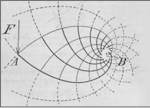
Figure 3.1 was used by Michell to explain the theory. The bolder continuous

trajectories are in compression and the lighter continuous trajectories are in tension. These

(22)

value F X length (AB) Frames whose bars coincide with these curves will represent minimum

quantity of material required. The dotted lines represent trajectories of principal strain where

material bars are not required.

Figure 3.1 Michell Truss Layout

Michell’s work was largely unnoticed for 50 years until Cox and Hemp realized the

importance of his findings and developed it further. Cox found exact solutions for an optimization problem based on Michell’s work and publish his findings in 1965 (20). Hemp

was credited with finding a correlation between Michell’s truss layout and the plastic

deformation of metals during operations such as die casting (21). The trajectories of plastic

(23)

3.2 Slip Lines

The lines in the middle of the Michell truss layout in tension are called alpha lines

and the ones in compression are called beta lines. Together, they are referred to as slip lines

and they are shown in Figure 3.2. Alpha and beta lines are always perpendicular to each other

at their points of intersection.

Figure 3.2 Alpha and Beta lines

Slip lines intersect the neutral axis at either a positive or negative angle of 45o. Any

number of slip lines can be used to describe a Michell truss layout. The coordinate system is

created with alpha and beta lines such that the angle of tangential stress τ is positive. The

angle of τ with respect to the alpha line is measured as θ. The relationship of θ with the

curvature of alpha and beta lines are described as

(24)

3.3 Correlation with Other Fields

As described above, once a correlation was found between slip line fields and the

lines of plastic deformation of metals, the interest in solving these topology problems grew.

Hemp developed an analytical method to derive slip line fields, but in general, complex

analytical expressions are needed especially when the geometry is not trivial.

It was found that these slip lines could be correlated with the plastic deformation field

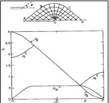
around a crack tip in the study of fracture mechanics as explained by Hutchinson in 1968

(22). He constructed a stress field centered at the crack tip. This field also had resemblance

with slip line fields initially developed by Michell. Perfectly plastic behavior was assumed

for these fields. Figure 3.3 below shows such a field for a plane strain case.

(25)

During the 1960’s, multiple numerical methods were derived to create slip line fields.

This coincided with the advent of computers and increased computing power. J. F. Ewing

developed a series method for constructing plastic slip line fields. He used a power series to

numerically approximate the slip line field (23). He defined the radii of curvature across the

field as a power series function of the different parameters and developed a numerical

solution. It was found that inverting the resulting equations to find the unknown coefficient

was difficult especially for complicated problems.

There is a small distinction in finding slip lines for optimum structures as opposed to

finding them for plane strain deformations. As described by Dewhurst (24), in the plane

strain metal deformation theory, the main area of focus was finding solutions to specific

boundary value problems for commonly used tool geometries such as die casting. In contrast

to designing structures with minimum weight, multiple examples can be developed for

unrestricted optimum structures.

3.4 Michell Theory Shortcomings

In 1973, Hemp (25) described some modifications needed to Michell’s theory and called them Michell’s optimality criteria in honor of the original work. Also, Hemp assumed

one permissible stress value for both compressive and tensile stresses. Examples of solutions

in which different permissible stresses are present were not given. This was followed by

Rozvany (2) demonstrated that Michell’s criteria is valid for all support conditions only if the

(26)

support conditions. Also, statically indeterminate loading conditions do not conform to

Michell’s optimality criteria. Michell’s truss exclusively optimizes two dimensional

structures in a plane stress condition.

In this section, a brief history of Michell Trusses including a description of slip lines

and their correlation with plastic strain was described including some of its shortcomings.

The following section reviews recent work in the field of topology optimization including an

(27)

4. REVIEW OF TOPOLOGY OPTIMIZATION

4.1 Categorizing Topology Optimization Methods

Topology optimization is the process of determining the connectivity, shape, and

location of voids inside a given domain (26). In the last two decades, there has been rapid

growth and continuous research in optimization techniques and it is an active area of research

in the field of structural and multidisciplinary optimization. In structural optimization, there

are a variety of different loading conditions. If the loading condition is similar to a pressure

vessel, it is design-dependent as well. One of the difficulties in shape optimization is that the

optimal shape may represent a multiply-connected set with internal boundaries whose

topology is not known and is difficult to determine because new internal boundaries cannot

be easily generated (27). There have also been exhaustive reviews conducted in this field.

This section provides a brief overview and discusses some specific methods.

The various methods of topology optimization can be broadly classified into two

specific groups as described by Srithongchai (28). The first is to change the size and layout

of trusses for a given number of nodes to achieve a specific design objective. In this method,

nodes that are too close to each other are merged together. Another approach couples a Finite

Element Analysis (FEA) code such as ANSYS with an optimization procedure. Density

values are modified based on the stress distributions. Regions of very low stress are removed

from the design altogether.

The specific methods gaining recent popularity are density-based methods called

(28)

(ESO). Within a fixed domain, the goal of the optimization problem is to identify whether

each element should contain a solid material or remain void (26). In most similar problems,

the objective function will be a volume to stiffness ratio or compliance, and constraints are

set on material usage and the physical model is represented in a discretized form. For this

method, the algorithm is often coupled with an FEA code. Such optimization techniques have

often resulted in a structure as shown in Figure 4.1 (29) as a discretized form. This specific

example also considered traditional manufacturing constraints.

Figure 4.1 Discretized ESO Optimized Structure Shape (29)

In the previous method for density variation calculation, density was a discrete

variable where each cell is either void or solid. Currently, research is being conducted using

material models which allow the density of the material to cover a complete range from 0

(void) to 1 (solid) where all intermediate values are also acceptable (30). This can be

achieved with a periodic perforated microstructural material whose density is a design

(29)

A bubble method was described by Eschenauer (31) about twenty years ago which is

included under the ESO method. An iterative positioning and a hierarchically structured

shape optimization for new holes were used. The boundaries were treated as parameters and

the shape of new bubbles was determined as a parametric optimization. Figure 4.2 shows the

initial design and the increasing size of the bubbles as it progresses towards the optimized

design.

(30)

The method chosen for topology optimization also changes based on the application.

Dentistry, biomedical, and aerospace applications have slight differences depending on

whether they are structural or aeronautical applications.

4.2 Coupling Optimization Methods with a Finite Element Code

Optimization algorithms are often coupled with finite element analysis code in the

pre- and post-processing steps. This thesis couples the ANSYS finite element code with an

optimization algorithm. In the following discussion, a review of recent research is given in

which a similar approach was taken.

A common problem with coupling a finite element code with an optimization method

is related to defining the mesh as the shape changes. In general, the definition of a finite

element mesh is a manual process that depends on an analyst’s past experience, knowledge

and intuition (32). It is difficult to automate this procedure when the geometry changes.

Nevertheless, this approach is commonly used for optimization analyses. A general approach

that works well when coupled with finite element analysis is hard-kill methods, such as ESO

methods. They work by gradually removing a finite amount of material from the design

domain (26). Bendsoe (33) also coupled finite element analysis and performed shape

optimization using the solid/void approach as previously described. The main goal was to

replace the discrete nature of the approach and introduce the density as a continuous design

variable. Zhou (27) solved a simple truss layout problem for compliance using an iterative

continuum-based optimality criteria (COC) method. A finite element program was combined

(31)

(34) who coupled a finite element code with an algorithm for shape and topology

optimization. They were able to find a numerical solution comparable with an analytical

solution for a Michell truss shape. A shape and topology optimization was conducted for

multiple loading scenarios as well. Another problem that frequently occurs when finite

element analysis is coupled with topology optimization is that the finite element model

experiences numerical singularities that do not exist in the physical model. This problem was

addressed by Jog (35). He suggested several strategies to stabilize solutions such as using

filters in post-processing operations.

4.3 Heuristic Approaches to Optimization

Optimization techniques can be broadly classified as either continuous or heuristic

techniques. For continuous functions, there are zeroth-order, first-order and second-order

information that are used by different techniques to find the optimum solution. Some

common approaches are the Golden section method, Powell’s method of conjugate direction,

BFGS, and the Augmented Lagrangian Method. These methods are derived from a common

principle in which the search direction at a starting point is determined by evaluating the

objective function so that it has a lower value and it travels the maximum amount in that

direction. This process is repeated until an optimum is reached. Note that this set of problems

can also incorporate multiple constraints.

Heuristic approaches are more suitable for black-box optimization. Some common

optimization techniques are Simulated Annealing, Genetic Algorithms, and Particle Swarm

(32)

clear pattern between the objective function at one point as compared to another. Heuristic

approaches try to refine the selected points based on information from a previous set of

results. These methods can accept discrete and continuous variables. One distinct

characteristic of heuristic approaches is that it is not known if the global optimum has been

reached. In addition, different simulations using the same algorithm may often yield different

results.

Genetic Algorithms use random number generation to find specific values for the

design variables and it progresses towards a solution without regard to how the function is

evaluated (36). The algorithm gets its name because of the similarity to genetics. A set of

designs is developed from random numbers which constitute the initial generation. Based on

the function values the fittest designs are selected, and are used to create ‘children’ or new

designs for a subsequent generation. Every generation also has some ‘mutated’ designs or

randomly generated designs. This approach is extremely flexible and is widely used in many

engineering disciplines for finding an optimum solution.

Another heuristic method is called Particle Swarm Optimization. This method is

similar to genetic algorithms in the fact that the initial set of designs is generated from

random numbers (37). Once the objective function is evaluated, a particular design or

‘particle’ remembers its coordinates in hyperspace. Each particle has a position and velocity.

The position and velocity of a given particle are dependent on the objective function value at

the current position as well as the objective function value of other particles at their

(33)

particle. In this manner, all particles move around the hyperspace and find the best fitness

(36).

Another popular heuristic method is called Simulated Annealing. Like its name, the

algorithm is inspired by the annealing process. A space might have multiple local minima

and if a design solution is stuck in such a local minimum, an algorithm must be able to accept

objective function values of greater value before descending to the global minimum. A

random point is evaluated initially. Then, a second point is evaluated and the objective

functions are compared. If the objective function is less, the new coordinates are accepted

and the objective function value is updated. If the objective function of the new point is

higher, then the new point is sometimes accepted and sometimes rejected. The acceptance is

dependent on the probability density function (PDF) of the Boltzmann distribution. If the

density is greater than a random value generated, the point is accepted. Otherwise, the

algorithm reverts to the previous point. As the number of iterations increases, the PDF

decreases and fewer unsatisfactory points are accepted (36).

This completes the review of the optimization concepts used in the thesis. In the

following chapters, these concepts are applied to a specific problem to achieve an optimum

(34)

5. PROBLEM DESCRIPTION

5.1 Overview of the Thesis

In the previous chapters, a review of the additive manufacturing (AM) industry was

described, and the concepts of a Michell truss layout and topology optimization were

discussed. As described in the Introduction, a technique to determine the topology of a part is

developed in this thesis. The topology is inspired by a Michell truss layout and optimized

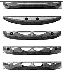
using an existing heuristic technique. Srithongchai created a design of a simply-supported

beam that was inspired by a Michell truss layout (28). A part was manufactured with a CNC

milling machine and several tests of the truss were conducted. This paper and its results are

presented in the following section and it forms the basis for this thesis. The results from

Srithongchai (28) are subsequently used to validate the technique developed in this thesis.

5.2 Summary of ‘A theoretical and experimental investigation of a family of minimum-weight simply-supported beams’ (28)

A summary of the paper ‘A theoretical and experimental investigation of a family of

minimum-weight simply-supported beams,’ authored by Sriruk Srithongchai, Murat

Demircubuk, and Peter Dewhurst is presented in this section (28). The Michell truss layout

described in this paper is used as a basis for demonstrating the optimization technique

developed in this thesis. The authors used a matrix method to find a solution for a

(35)

tested and deflections were compared with theoretical results. The subject is a symmetrical

beam case study as shown in Figure 5.1.

Figure 5.1 Symmetrical Simply-Supported Beam (28)

The joint coordinates are shown below in Table 5.1. Note that these numbers are

rounded off to the nearest hundredth. The dimensions are based on a height of unit length and

so they may be scaled accordingly.

Table 5.1: Unit Joint Coordinates (28)

J0 J11 J12 J13 J14 J15 J22 J23

(0,1) (0,0) (0.38,0.08) (0.71,0.29) (0.92,0.61) (1,1) (0.4,0) (0.85,0.09)

J24 J25 J33 J34 J35 J44 J45 J55

(36)

For a unit load applied at the location shown above in Figure 5.1, the reaction forces

in each of the tension and compression members to the left of the joint are shown in Table

5.2. These numbers are also rounded to the nearest hundredth and will be used to validate of

the beam model in Section 5.5.

Table 5.2 Reaction Forces for Unit Load (28)

J0 J11 J12 J13 J14 J15

- (0,-0.08) (0.22,-0.16) (0.21,-0.27) (0.18,-0.31) (0.13,-0.67)

J22 J23 J24 J25 J33 J34

(0.98,-0.08) (0.37,-0.19) (0.32,-0.25) (0.25,-0.65) (0.60,-0.05) (0.26,-0.14)

J35 J44 J45 J55

(0.23,-0.60) (0.33,-0.04) (0.19,-0.56) (0.13,-0.52)

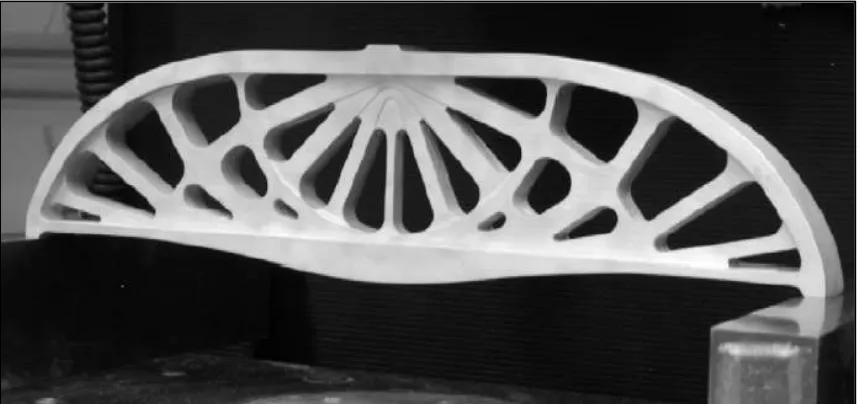
As described previously, the beam was machined with a CNC mill and the cross

section is similar to the one shown in Figure 5.1. A photograph of this beam is shown in

Figure 5.2. The depth is 25mm, the span of the entire beam is 350 mm, and the volume is 275

cm3. The beam was made of 6061 T6 Aluminum which has a yield strength of 276 MPa.

Tests conducted on this beam which was balanced on the two ends in order to restrain

the downward movement. A force was applied in the downward direction at the center. A

maximum stress of 260 MPa was assumed before yielding. It was calculated that in the

(37)

reports the overall volume of the optimized truss, but no specific thickness for each strut in

the truss is provided.

Figure 5.2 Image of Symmetrical Simply-Supported beam (28)

Reference (28) provides two important graphs to describe the properties of the

simply-supported beam. Figure 5.3 shows the strain as a function of the stress applied. This

graph shows non-linear behavior near and after 276 MPa which is the yield strength of the

material. The slope of the linear region is used to calculate the elastic modulus as 74265

(38)

Figure 5.3 Stress-Strain Curve of Simply-Supported Beam

The deflection is shown in Figure 5.4. The maximum deflection occurs close to the

bottom left of the beam and it is experimentally calculated. The experimental results were

obtained through a load test. The deflection was calculated for different loads. For a load of

98.5KN a deflection of 2.54 mm was expected. This was considered the maximum load

before non-linear behavior occurred. The test was halted at the onset of buckling.

(39)

In the following chapters, the optimum design of a Michell truss is found using the

optimization technique developed in this thesis. The optimum design is validated using the

results of Reference (28).

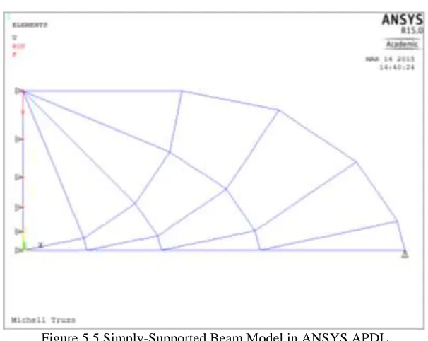
5.3 FEA Model of a Simply-Supported Beam

For the model described Reference (28), a finite element model of the symmetrical

simply-supported beam was created. The objective is to couple an optimization algorithm

with the FE model in the pre- and post-processing stage so that the mass of the beam can be

minimized. The ANSYS APDL software was used since it is a widely accepted industry

standard FE code. In the following section, the ANSYS model is explained in detail. The

details of coupling it with an optimization algorithm are discussed in Chapter 7.

(40)

The simply-supported beam is modeled as a linear elastic material using BEAM3

elements. The ANSYS model is shown in Figure 5.5. Half the beam is modelled and a

symmetric boundary condition is applied on the other half. The force applied is halved to

account for this symmetry. The Keypoints are defined at locations as described in Reference

(28) as shown in Table 5.1. For each unit length of 1, an equivalent distance of 72.91 mm

was taken in accordance with the dimensions listed in Reference (28). For the ANSYS

model, half-span of the beam is 175 mm. The Keypoints are connected by lines.

5.4 Boundary Conditions

Figure 5.2 shows constraints on the bottom right and left ends of the symmetrical

simply-supported beam which prevent it from moving down. This is modelled by applying a

constraint on the bottom right keypoint and preventing it from moving in the vertically. To

account for symmetry, the line on the left is not allowed to move horizontally. A downward

force is applied at the top left keypoint. A force of half the magnitude is applied to account

for the symmetry condition.

The ANSYS model is coupled with and controlled by an optimization algorithm. The

boundary conditions as well as other model parameters such as the depth, location of the

keypoints and the lines connecting these keypoints are held constant. The input for the

ANSYS model is defined in a text file. For a given design, the only variable in the model is

the thickness of each of the lines. The optimization algorithm will be used to determine the

optimal thickness of each of the lines. The moment of inertia and the cross section of each

(41)

section the results for this ANSYS model as well as other post-processing steps are

described.

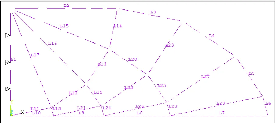
5.5 Validation of the Beam Model

The model was validated by comparing the internal forces of each of the members

with the published forces in Reference (28). The boundary conditions described in the

previous section were applied and a force of 0.5 N (half of a unit load to account for

symmetry) was used. The areas and thicknesses were set to unity as well. The line numbers

that will be used for comparison with Reference (28) are shown in Figure 5.6. The model was

then solved to determine the optimal member thicknesses.

(42)

Once the model was solved, the axial stress values across the model were obtained.

The axial stress shown in Table 5.3 is constant along a line.

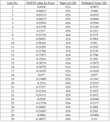
Table 5.3 Comparison of Internal Forces for ANSYS Model and Published Results (28)

Line No. ANSYS value for Force Paper ref (28) Published Value (28)

1 -0.0438 J11c -0.0875

2 -0.66613 J15c -0.666

3 -0.65333 J25c -0.6532

4 -0.60473 J35c -0.6046

5 -0.55943 J45c -0.5594

6 -0.51705 J55c -0.5169

7 0.1317 J55t 0.1321

8 0.32729 J44t 0.3275

9 0.59653 J33t 0.5965

10 0.98102 J22t 0.981

11 0.22429 J12t 0.2243

12 0.21396 J13t 0.2139

13 0.17873 J14t 0.1786

14 0.13016 J15t 0.1301

15 -0.30714 J14c -0.3072

16 -0.26752 J13c -0.2676

17 -0.16187 J12c -0.1618

18 -0.077 J22c -0.077

19 -0.19409 J23c -0.1941

20 -0.2514 J24c -0.2515

21 0.37217 J23t 0.3722

22 0.32336 J24t 0.3253

23 0.24712 J25t 0.2472

24 -0.0549 J33c -0.0548

25 -0.13756 J34c -0.1377

26 0.26065 J34t 0.2604

27 0.22645 J35t 0.2261

28 -0.0404 J44c -0.0406

(43)

For the joints shown in Table 5.3, a subscript ‘c’ denotes a compression member to

the left of the joint as shown by the dotted line in Figure 5.2. The subscript ‘t’ is used to

denote a member in tension as shown by a solid line in the same figure. The internal forces

in the numerical model show excellent agreement with the published results except for the

first line. This value is exactly half because the numerical model represents half the value of

the actual thickness of the line. Hence, it can be concluded that the ANSYS numerical model

is similar to the model described in Reference (28).

5.6 Post Processing of the Finite Element Model

The model described in the previous section was used to compute the following

results. For a constant thickness value of 10 mm for all struts of the beam, the deformed

(44)

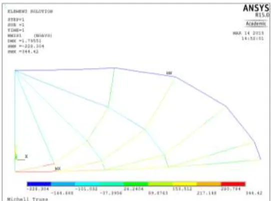
Figure 5.7 Deformed Shape of Simply-Supported Beam Model (blue)

The blue solid lines represent the deformed shape and the black line is the

un-deformed shape. As expected, the left side of the beam model deforms in the negative

y-direction because of the force applied at the top left corner in the downward y-direction. The

maximum deflection for this model is 1.93 mm. Note that the deflection for the constant

thickness of 10 mm are expected to be stiffer than the tested model. Since the beam is

represented by beam elements, some of the struts might have overlapping material.

The outputs of interest are the maximum and minimum stress of each strut. The

maximum stress is found by adding the axial and bending stresses and the minimum stress is

found by adding the two stresses as if they were compressive. Figure 5.8 shows the

maximum stress throughout the model. It is important to note that the stress numbers that

exceed the yield stress limit are inaccurate because the model is based on the assumption that

the material is linear elastic. Therefore, the only valid conclusion is that the stresses exceed

(45)

Figure 5.8 Maximum Stress in Simply-Supported Beam Model

As expected, the alpha lines are in tension and have tensile stresses. Some struts in

the beam are stressed above the yield limit as well. The element stresses are stored in a text

file and read back to MATLAB for each design evaluation in the optimization algorithm. The

initial thickness value of 10 mm is not optimized.

5.7 Summary

The Srithongchai paper (28) was reviewed and a finite element model of a

simply-supported beam was described. The deformed shape and maximum stress value was found

for a constant thickness of 10 mm for all struts. Note that the struts are represented by lines

for which the cross sectional area and moment of inertia are defined. The beam model was

validated by comparing the internal forces with the published values in Table 5.2. In the next

(46)

6. GENERAL STRUCTURAL LAYOUT OF A MICHELL TRUSS

6.1 Principal Stress Trajectories for a Simply-Supported Beam

To find the optimum topology for a given design, the layout of the Michell truss is

first determined by describing the location and direction of the slip lines throughout the field.

As described in Chapter Two, the slip lines represent the directions of the principal stresses

throughout the field. However, the slip line trajectories are tedious to find. Melchers (38)

recently described extending the range of Michell-like optimal topology structures by

showing slip line layouts for different loading conditions. To define complex equations,

numerical and analytical methods have been developed to find the slip lines for relatively

well-defined problems such as a simply-supported beam and a cantilever beam. The Matrix

method (39) and the Ewing Power Series (23) method are two such examples. These

techniques result in complex equations and a simpler method is needed to define the layout

of a Michell truss.

In a recent paper on optimum structural design, Barnett found that the members in an

optimum structure must lie along the lines of principal strain. Otherwise, a direction could be

found at a point on a member for which the direct strain had a magnitude greater than the

current strain (40). Timoshenko (41) also discusses the trajectories of principal stress for

plane stress applications. The trajectories of the principal stresses for a simply-supported

beam with uniform loading are shown in Figure 6.1. Note that the trajectories coincide with

the direction of the principal stress at a given point. The magnitude of the principal stress is

(47)

Figure 6.1 Principal Stress Trajectories for a Simply-Supported Beam (41)

6.2 Principal Stress Trajectories using Finite Element Analysis

As discussed in the previous section, it is known that the principal stress trajectories

for a given loading condition coincide with the direction of the slip lines. The topology of the

model and the exact placement of material is the central objective for optimization. These

slip lines which define the position of material can also be derived by creating a finite

element model of the outside periphery of the design. Once the principal stress trajectories

are obtained from such an analysis, the slip lines can be constructed to create the internal

geometry of the lattice structure. The simply-supported beam described in Chapter 5 is used

in this thesis to demonstrate this correlation. The Michell truss in Reference (28) is also used

(48)

6.3 CAD Model and FEA Model

A Computer Aided Design (CAD) model of the simply-supported beam was created

in SolidWorks using the dimensions described in Chapter 5. The outer boundary of the beam

was modeled while the interior region of the beam was treated as a complete solid.

Figure 6.2 Finite Element Model Showing Constraints and Loads for Simply-Supported Beam

Figure 6.2 shows the overall geometry of the beam. Only half of the beam is modeled

and a symmetry condition is used along the left edge. The right bottom point is fixed in the

vertical direction representing a constraint on the model. The left top most point is the

location of the force. To account for symmetry the left-most edge is not allowed to move

(49)

are used. The material is aluminum 6061 T6 which has a yield strength of 276 MPa, an

elastic modulus of 6.9e4 N/mm2, and a Poisson ratio of 0.33.

Figure 6.3 Original Michell Paper Example (3)

For a cantilever beam, the initial shape of the Michell truss is shown in Figure 6.3

(28). The force is applied at point A and point B is fixed. Figure 6.4 shows the geometry as

setup in SolidWorks Simulation. A force is applied on the left and the right face is fixed.

Triangular elements are used and the material is aluminum. The results for this model are

(50)

Figure 6.4 Finite Element Model Setup for 2nd Model

6.4 Plane Stress Model Results and Discussion

The principal stress trajectories for this finite element model are shown in Figure 6.5.

Based on the initial shape as described by the experimental results, a separate Michell truss

CAD model was created and this is superimposed in this figure. Note that the trajectories

align with the direction of the Michell truss struts and the slip lines. As shown, the principal

stress trajectories align with the alpha and beta lines of the internal lattice structure of the

model in Reference (28). There are large stresses near the support which is indicated with a

large arrow. These large stresses are ignored in this analysis. Note that the lines and

(51)

Figure 6.5 Maximum and Minimum Principal Stress Trajectories Superimposed on the CAD Model

The stress trajectories for the beam described in Michell 1904 (3) paper is shown in

Figure 6.6. The slip lines in Reference (3) align with the principal stress trajectories as found

(52)

Figure 6.6 Slip Lines Trajectories Superimposed for 2nd Model

As shown in the previous results, the principal stress trajectories are a positive

indication of the placement of struts on the interior of the beam. This method does not

(53)

manufacturing limitations. The thickness of each of the line is also unknown. This results in

the stiffest structure for a given mass. As explained in Chapter 2, Michell trusses have certain

limitation. The yield strength in compression and tension must be the same and plane stress

conditions must be satisfied. These assumptions are adhered to when creating the finite

element model used in the above examples.

Since the stress along each line can change, an optimization algorithm is needed to

find the appropriate thickness for each slip line. The next chapter describes the optimization

(54)

7. OPTIMIZATION ALGORITHM

7.1 Introduction

In Chapter 4, several common topology optimization techniques were reviewed. In

this thesis, a Michell truss is assumed to represent an optimum layout of a lattice structure.

This initial shape is found using directions of the principal stresses trajectories. It is

important to note that the stresses are not uniform along the principal stress trajectories. The

stress values are also dependent on the thickness and area of each strut in the lattice. The

mass is also dependent on the area of each strut. A heuristic technique called simulated

annealing is used to find the thickness of each strut in the lattice so that the mass is

minimized. In this chapter, the optimization problem is formulated and the parameters used

in the algorithm are described.

7.2 Method Formulation of the Optimization Problem

The objective of the optimization problem is to minimize the mass without violating

any of the constraints. One such constraint is that the maximum allowable stress for all struts

of the beam be less than the yield strength (𝜎_𝑦). ANSYS was used to calculate stress. A

description of the ANSYS model was provided in Chapter 5. The thicknesses of each strut in

the lattice constitute the design variables of the optimization problem. The optimization

(55)

Minimize: 𝑀𝑎𝑠𝑠 = 𝜌 ∗ 𝑑𝑒𝑝𝑡ℎ ∗ ∑(𝑙𝑒𝑛𝑔𝑡ℎ ( 𝑖 ) ∗ 𝑡ℎ𝑖𝑐𝑘𝑛𝑒𝑠𝑠 ( 𝑖 ))

Subject to: 𝑆𝑡𝑟𝑒𝑠𝑠 𝑣𝑎𝑙𝑢𝑒 ( 𝑖 ) − 𝜎_𝑦 <= 0

𝑇ℎ𝑖𝑐𝑘𝑛𝑒𝑠𝑠 ( 𝑖 ) > 0

Where ‘i’ represents the number of design variables and is equal to the number of

struts in the ANSYS model. The simply-supported ANSYS beam model has 29 struts. The

length of all lines is constant and static during the optimization. In Chapter 4, various

methods commonly employed for topology optimization were described. In this thesis, the

optimization algorithm is coupled with a finite element model.

7. 3 Method: Description of the Algorithm

To optimize the thickness of each strut a simulated annealing optimization algorithm

was developed using MATLAB and then coupled with the ANSYS finite element analysis

software. There are 29 lines in the ANSYS model and a uniform thickness is assumed along

each line. Hence, there are 29 thickness values to be determined using the optimization

(56)

Figure 7.1 Flowchart for Simulated Annealing Algorithm

An initial design of thickness values for all of the struts is entered. This initial design

is a constant thickness value of 5, 10, or 15 mm for all struts. Based on the length, depth and

density of each strut, the volume and mass of a current design can be calculated. The stress

values for the constraints are calculated in ANSYS as described earlier and read back into

MATLAB. The maximum and minimum stresses are determined and the absolute value is

found. Then, the maximum values of these two stresses are established. The difference of any

stress value and the yield strength is added as a penalty if it is above the yield strength. This penalty is multiplied by an ‘rp’ factor. The overall objective of the algorithm is to minimize

(57)

𝐹𝑖𝑡𝑛𝑒𝑠𝑠 = 𝑀𝑎𝑠𝑠 + 𝑃𝑒𝑛𝑎𝑙𝑡𝑦 ∗ 𝑟𝑝

The penalty and mass calculations are defined above. The ‘rp’ value changes as the

algorithm progresses and it will be explained in the following discussion.

7.4 Generating a New Design

Once the initial fitness is calculated, the counter for the number of iterations and

design evaluations per iteration begins. A new design is generated and the fitness values are

compared. To generate a new design a varied approach is used. If there are stress violations

(and subsequently penalty) in the previous fittest design held, a new design is created by

randomly selecting ten thickness values and perturbing it. For a selected thickness value, if

the corresponding stress in that strut in the previous design is above the yield strength, the

new thickness will increase in value between 0 and 1 of the previously held value.

𝑛𝑒𝑤 𝑡ℎ𝑖𝑐𝑘𝑛𝑒𝑠𝑠𝑣𝑎𝑙𝑢𝑒(𝑖) = 𝑡ℎ𝑖𝑐𝑘𝑛𝑒𝑠𝑠𝑣𝑎𝑙𝑢𝑒(𝑖) + 𝑟𝑎𝑛𝑑

Where ‘rand’ is a random number between 0 and 1. For the selected thickness, if the

corresponding stress is below the yield strength, the new thickness can be perturbed upwards

or downwards.

𝑛𝑒𝑤 𝑡ℎ𝑖𝑐𝑘𝑛𝑒𝑠𝑠𝑣𝑎𝑙𝑢𝑒(𝑖) = 𝑡ℎ𝑖𝑐𝑘𝑛𝑒𝑠𝑠𝑣𝑎𝑙𝑢𝑒(𝑖) − 0.5 + 𝑟𝑎𝑛𝑑

The thickness is allowed to increase or decrease because the stress values of all struts

(58)

may still be below the yield strength, but the stress of an adjoining strut might increase above

the allowable limit.

If all stress values are below yield for the previous fittest design, a different approach

for design creation is used. Only one thickness value is selected out of 29 and it is changed as

follows:

𝑛𝑒𝑤 𝑡ℎ𝑖𝑐𝑘𝑛𝑒𝑠𝑠𝑣𝑎𝑙𝑢𝑒(𝑖) = 𝑡ℎ𝑖𝑐𝑘𝑛𝑒𝑠𝑠𝑣𝑎𝑙𝑢𝑒(𝑖) − 0.7 + 𝑟𝑎𝑛𝑑

Since the stress values of all struts are below yield, the selected member has a higher

probability of decreasing in value based on the above equation. This approach was selected

based on parameters from research on topology optimization using simulated annealing (42).

7.5 Accepting a New Design

Once a new fitness is calculated based on the new design described above, it is

compared to the existing fittest design. If the fitness of the new design is lower, it replaces

the existing design as the new fittest design and its thickness values are stored.

If the new design does not have a lower fitness, its acceptance is dependent on a

probability density function (PDF). This value ‘p’ is determined by the following equation:

𝑝 = 𝑒

𝑑𝑒𝑙𝑡𝑎_𝑒𝑡

Where 𝑑𝑒𝑙𝑡𝑎_𝑒 = 𝑓𝑖𝑡𝑛𝑒𝑠𝑠 − 𝑛𝑒𝑤 𝑓𝑖𝑡𝑛𝑒𝑠𝑠

(59)

‘delta_e’ is a negative value when the new fitness is higher than the existing fittest

design. The value of ‘p’ is always between 0 and 1 when calculated as described above. This

value is compared to a random number generated by Matlab between 0 and 1. If ‘p’ is higher,

the bad design replaces the current fittest design; and if ‘p’ is lower, the algorithm continues

with the previously held fittest design. The process of accepting bad designs with higher

fitness values allows the algorithm to escape local minimums.

7.6 Cooling Schedule

The temperature ‘t’ for a given iteration determines the value of ‘p’ and subsequently

the probability of accepting a bad design. As the number of iterations increase, the

probability of accepting bad designs decreases. The temperature is initially set to 60 and

decreases by a factor of 0.990. Hence, for all designs evaluated at a given iteration, the

probability of accepting bad designs is held constant. Then, as the iteration number increases,

the temperature decreases. The probability of accepting a bad design for the next set of

design evaluations will decrease.

In this chapter, the optimization problem was presented and the procedure of the

simulated annealing algorithm was described. The objective of the algorithm is to reduce the

fitness or minimize mass with constraints being accounted for by using a penalty function. In

the following chapter, additive manufacturing constraints are discussed and how they are also

(60)

8. CONSTRAINTS FOR ADDITIVE MANUFACTURING

8.1 Introduction

In the previous chapter, an optimization algorithm was described for determining the

thickness for each strut in the symmetrical simply-supported beam. In this chapter,

constraints for additive manufacturing (AM) will be explained followed by the method for

incorporating these constraints into the algorithm.

Additive manufacturing gives a designer the freedom to design and manufacture

complex parts with higher stiffness and less mass as compared with parts that are made with

traditional manufacturing processes. As discussed in Chapter 2, additively manufactured

parts are successfully replacing multiple components in an assembly and transferring loads

within a structure with greater efficiency.

Constraints for additive manufactured parts are highly dependent on the specific

process. These manufacturing constraints need to be taken into account when designing a

part. Constraints vary based on the material, machine and processes. The design constraints

can also be affected by the use of support material in some machines. It is probable that AM

machines, materials and processes will continue to improve over time and this will further

reduce manufacturing constraints. There have been optimization algorithms in previous

research that investigate minimum member thickness constraints (43). However, there has

been no research on methods to incorporate specific AM constraints into the topology

optimization process. In this thesis, the algorithm described in Chapter 7 will be modified to