Qsparse-local-SGD: Communication Efficient Distributed SGD with Quantization, Sparsification, and Local Computations

(1)

UCLA

UCLA Electronic Theses and Dissertations

Permalink https://escholarship.org/uc/item/4215t5ht Author Basu, Debraj Publication Date 2019 Peer reviewed|Thesis/dissertation

(2)

UNIVERSITY OF CALIFORNIA Los Angeles

Qsparse-local-SGD:

Communication Efficient Distributed SGD with Quantization, Sparsification, and Local Computations

A thesis submitted in partial satisfaction of the requirements for the degree

Master of Science in Electrical and Computer Engineering by

Debraj Debashish Basu

(3)

(4)

ABSTRACT OF THE THESIS Qsparse-local-SGD:

Communication Efficient Distributed SGD with Quantization, Sparsification, and Local Computations

by

Debraj Debashish Basu

Master of Science in Electrical and Computer Engineering University of California, Los Angeles, 2019

Professor Suhas N. Diggavi, Chair

Large scale distributed optimization has become increasingly important with the emergence of edge computation architectures such as in the federated learning setup, where large amounts of data, possibly of a secure nature and generated in an online manner can be massively distributed across personal devices. A key bottleneck for many such large-scale problems is in the communication overhead of exchanging information between devices over bandwidth limited networks as well as in the unreliability of communication for distributed optimization. The existing approaches propose to mitigate these bottlenecks either by using different forms of compression or by computing local models and mixing them iteratively. In this thesis we first propose a novel class of highly communication efficient operators that em-ploy stochastic and deterministic quantization with aggressive sparsification such as Top-k

in the form of a composed operator. Furthermore, in federated learning one can use local computations to reduce communication. Using such a framework, we incorporate local it-erations into our algorithm which allows the communication to be infrequent and possibly asynchronous thereby enabling significantly reduced communication.

Putting them together we have distributed Qsparse-local-SGD for federated learning for

(5)

we observe that quantization and sparsification are almost for “free” for smooth functions, both non-convex and convex. We characterize the asymptotic allowable limits of local it-erations for synchronous and asynchronous implementations of Qsparse-local-SGD, so as to

harness both the distributed processing gains as well as the benefits of quantization, sparsifi-cation and local computations. Our numerics demonstrate thatQsparse-local-SGD combines

the bit savings of our composed operators, as well as local computations, thereby outper-forming the cases where these techniques are individually used. We use it to train ResNet-50 on ImageNet, as well as a softmax multi-class classifier on MNIST, resulting in significant savings over the state-of-the-art, in the number of bits transmitted to reach target accuracy.

(6)

The thesis of Debraj Debashish Basu is approved.

Christina Panagio Fragouli Lieven Vandenberghe

Suhas N. Diggavi, Committee Chair

University of California, Los Angeles 2019

(7)

(8)

TABLE OF CONTENTS 1 Introduction . . . 1 1.1 Related Work . . . 2 1.2 Contributions . . . 4 1.3 Organization . . . 5 1.4 Preliminaries . . . 6

1.4.1 Smoothness and Convexity . . . 6

1.4.2 Useful Vector Inequalities . . . 7

2 Communication Efficient Operators . . . 8

2.1 Quantization . . . 8

2.2 Sparsification . . . 10

2.3 Composed Operators . . . 11

2.4 Discussion . . . 14

3 Distributed Synchronous Operation . . . 15

3.1 Qsparse-local-SGD . . . 15

3.2 Assumptions . . . 17

3.3 Error Compensation . . . 17

3.3.1 Decaying Learning Rate . . . 18

3.3.2 Fixed Learning Rate . . . 19

3.4 Main Results . . . 19

3.5 Proof Outline . . . 21

(9)

3.5.2 Proof outline of Theorem 2 . . . 23

4 Distributed Asynchronous Operation . . . 25

4.1 Asynchronous Operation . . . 25

4.2 Main Results . . . 27

4.3 Proof Outline . . . 28

5 Communication Cost and Experiments . . . 31

5.1 Communication Cost . . . 31

5.2 Summary of Results . . . 33

5.3 Non Convex Objective . . . 34

5.3.1 Experiment setup . . . 34

5.3.2 Results . . . 34

5.4 Convex Objective . . . 35

5.4.1 Model Architecture . . . 36

5.4.2 Parameter selection and Learning rates . . . 36

5.4.3 Experiment Results . . . 37

6 Conclusion . . . 40

A Supplementary material for preliminaries in Chapter 1 . . . 41

B Supplementary material for Chapter 2 . . . 44

B.1 Proof of Lemma 1 . . . 44

(10)

B.3 Proof of Lemma 3 . . . 47

C Supplementary material for Chapter 3 . . . 50

C.1 Proof of Lemma 4 . . . 50

C.6 Smooth Objective: Proof of Theorem 1 . . . 56

C.7 Convex Objective: Proof of Theorem 2 . . . 59

D Supplementary material for Chapter 4 . . . 64

D.1 Proof of Lemma 9 . . . 64

E Supplementary material with additional results . . . 71

E.1 Synchronous . . . 71

E.2 Asynchronous . . . 71

E.3 Proof of Theorem 5 . . . 72

(11)

LIST OF FIGURES

5.1 Figures 5.1a-5.1c demonstrate the performance of our scheme in comparison with

ef-signSGD [KRS19], TopK-SGD [SCJ18,AHJ18] and local SGD [Sti19,YYZ18]

in a non convex setting. . . 35 5.2 Figures 5.2a-5.2c demonstrate the performance of our scheme in comparison with

ef-signSGD [KRS19] and TopK-SGD [SCJ18, AHJ18] in a convex setting for

synchronous updates. Here for H = 1,4,8,16, corresponds to the Algorithm 1

running with a synchronization period of at most H. . . 37

5.3 Figures 5.3a-5.3b demonstrate the performance of our scheme in comparison with

ef-signSGD [KRS19] and TopK-SGD [SCJ18, AHJ18] in a convex setting for

(12)

LIST OF TABLES

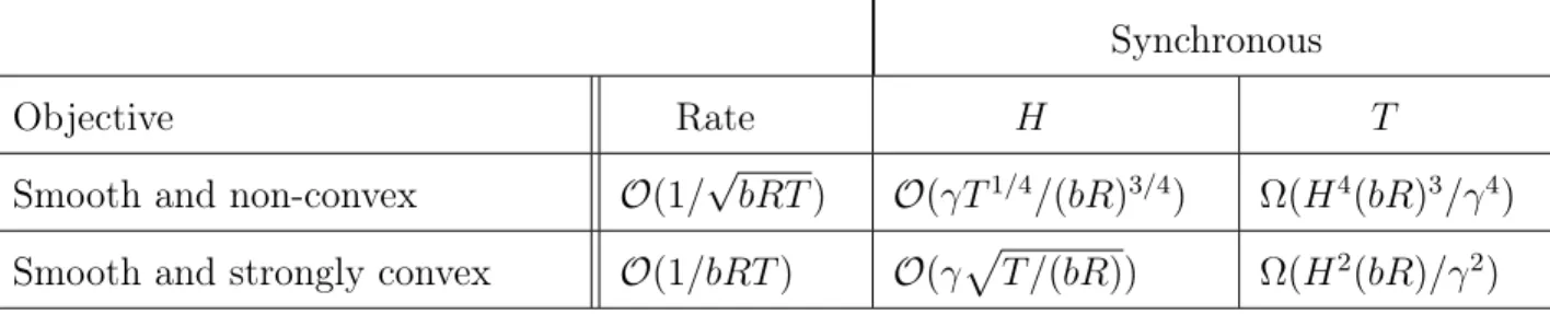
5.1 Summary of results for the synchronous setting with fixed learning rate in both the smooth and non-convex case and decaying learning rate in the smooth and strongly convex case. . . 33 5.2 Summary of results for the asynchronous setting with fixed learning rate in both

the smooth and non-convex case and decaying learning rate in the smooth and strongly convex case. . . 33

(13)

ACKNOWLEDGMENTS

My experience as a Masters student at UCLA has been exceedingly enriching, for which I am most grateful to my advisor, Professor Suhas Diggavi. I would like to thank him for his patience, generosity and unparalleled guidance over this duration. None of this would have been possible without his encouragement and support in many forms, for which I shall always remain indebted to him. Much of the contents of this thesis are a result of the foundations which were laid in classes offered by members of my thesis committee, Professor Diggavi, Professor Vandenberghe and Professor Fragouli, all of which truly inspired me and I thoroughly enjoyed them, both as a student, as well as a teaching assistant.

I have also had the privilege of enjoying the intellectual company of Dr. Deepesh Data and Dr. Can Karakus among many others, whose role has been critical in shaping this thesis. It has been an incredible journey undertaking research in collaboration with Deepesh, who has been a great mentor and friend, and whose expertise in several domains facilitated both our learning processes, eventually culminating in this thesis. I am also much obliged to Can, who not only introduced me to this area of research at the intersection of communication theory and machine learning, but always encouraged me to identify the right problem, and to make mistakes and learn from them. A special mention for Can, who has very kindly invested a lot of time around his other professional commitments without which this thesis would not have been possible.

I must admit that I have been very lucky throughout this journey. I would like to thank UCLA for the amazing curriculum that it offers which perfectly aligned with my interests in optimization, information theory and automated reasoning. As a teaching assistant, I have also had the opportunity of interacting with members of the faculty, as well as numerous graduate and undergraduate students, with different backgrounds. This diverse interaction, provided me with different perspectives for analyzing problems, and further enhanced my learning process. This is probably one of the things that I am going to miss the most about my time spent at UCLA.

(14)

I would like to also acknowledge several insightful discussions with Navjot in the early stages of this work, as well as the lunch and coffee breaks with Dhaivat, Navjot and Deepesh, which I would keep looking forward to each day. I must also mention all my labmates and friends, Deepesh, Mehrdad, Dhaivat, Navjot, Kenny, Sundar, Antonious, Osama, Yahya, Gaurav and Karmoose with whom I have had academic and friendly interactions and I wish them the very best for their current and future endeavors.

I would like to thank Sakshi, for her support, encouragement, and for being an amazing girlfriend. I am very proud of her. And finally I would like to thank my parents, Debashis and Areta who have been constant pillars of support throughout my life. Their immeasurable love and wisdom has been the driving force in my decisions and has always guided me well.

(15)

CHAPTER 1 Introduction

Stochastic Gradient Descent (SGD) [HM51] and its many variants have become the workhorse for modern large-scale optimization as applied to machine learning [Bot10,BM11]. We con-sider the setup in which SGD is applied to the distributed setting, where R different nodes

compute local stochastic gradients on their own datasets Dr. Co-ordination between them

is done by aggregating these local computations to update the overall parameter xt as,

xt+1 =xt− ηt R R X r=1 gr_t. where {g_tr}R

r=1 are the local stochastic gradients at the R machines for a local loss function

f(r)₍_x₎_{of the parameters, where} _f(r)_:

Rd→R and ηt is the learning rate.

The training of high dimensional models is done at a large scale over bandwidth limited networks. Therefore despite the distributed processing gains, it is well understood by now that exchange of full-precision gradients between nodes, causes communication to be the bot-tleneck for many large scale models [AHJ18,WXY17,BWA18,SYK17]. For example, consider training the ResNet 152 architecture [HZR16] which has about 60 million parameters, on the ImageNet dataset that contains 14 million images. Each full precision exchange between workers is around 0.24 GB. And this problem is at a much smaller scale in comparison to the real world platforms where data resides on personal devices such as laptops and tablets. Therefore the communication bottleneck could be significant in emerging edge computation architectures suggested by federated learning [Kon17, MMR17, ABC16]. To address this, many methods have been proposed recently, and these methods are broadly based on three major approaches:

(16)

1. Quantization of gradients, where nodes locally quantize the gradient (perhaps with

randomization) to a small number of bits [AGL17,BWA18,WHH18,WXY17,SYK17]. 2. Sparsification of gradients, e.g., where nodes locally selectTop_k values of the gradient

in absolute value and transmit these at full precision [Str15, AH17, SCJ18, AHJ18, WHH18,LHM18], while maintaining errors in local nodes for later compensation. 3. Skipping communication rounds whereby nodes average their models after locally

up-dating their models for several steps [YYZ18,Cop15,ZDW13,Sti19,CH16,WJ18]. In this work we proposeQsparse-local-SGDalgorithm, which combines aggressive

sparsifi-cation with quantization and local computations, along with error compensation, by keeping track of the difference between the true and compressed gradients. We propose both syn-chronous and asynsyn-chronous implementations of Qsparse-local-SGD in a distributed setting

where the nodes perform computations on their local datasets. In our asynchronous model, the distributed nodes’ iterates evolve at the same rate, but update the gradients at arbitrary times; see Chapter 4 for more details. We analyze convergence forQsparse-local-SGD in the distributed case, for smooth non-convex and convex objective functions. We demonstrate

that,Qsparse-local-SGD converges at the same rate as vanilla distributed SGD for many

im-portant classes of sparsifiers and quantizers. We implementQsparse-local-SGDfor ResNet-50

using the ImageNet dataset, and for a softmax multiclass classifier using the MNIST dataset, and show that we achieve target accuracies with about a factor of 15-20 savings over the state-of-the-art [AHJ18,SCJ18,Sti19], in the total number of bits transmitted.

1.1 Related Work

The use of quantization for communication efficient gradient methods has decades rich history [GMT73] and its recent use in training deep neural networks [SFD14, Str15] has re-ignited interest. Theoretically justified gradient compression using unbiased stochastic quantizers has been proposed and analyzed in [AGL17, WXY17, SYK17]. Though methods

(17)

in [WWL18, WSL18] use induced sparsity in the quantized gradients, explicitly sparsifying the gradients more aggressively by retaining Top_k components, e.g., k <1%, has been

pro-posed [Str15, AH17, LHM18, AHJ18, SCJ18], combined with error compensation to ensure that all co-ordinates do get eventually updated as needed. [WHH18] analyzed error compen-sation for QSGD, without Top_k sparsification and a focus on quadratic functions. Another

approach for mitigating the communication bottlenecks is by having infrequent communi-cation, which has been popularly referred to in the literature as iterative parameter mixing,

see [Cop15], and model averaging, see [Sti19, YYZ18, ZSM16] and references therein. With

the onset of powerful processing units such as graphics and tensor processing units, increas-ing the computation to communication ratio would enable distributed algorithms to converge faster. Furthermore, this would also be useful in applications where compression does not re-sult in significant gains, such as in cloud computing based frameworks where the data resides online and the computations are also performed online. Our work is most closely related to and builds on the recent theoretical results in [AHJ18,SCJ18,Sti19,YYZ18]. [SCJ18] consid-ered the analysis for the centralizedTop_k (among other sparsifiers), and [AHJ18] analyzed a

distributed version with the assumption of closeness of the aggregatedTop_k gradients to the

centralizedTop_kcase, see Assumption 1 in [AHJ18]. [Sti19,YYZ18] studied local-SGD, where

several local iterations are done before sending thefull gradients, and did not do any gradient

compression beyond local iterations. Our work generalizes these works in several ways. We prove convergence for thedistributed sparsification and error compensation algorithm,

with-out the assumption of [AHJ18], by using the perturbed iterate methods [MPP17, SCJ18]. We analyze non-convex (smooth) objectives as well as strongly convex objectives for the distributed case with local computations. [SCJ18] gave a proof of sparsified SGD, for convex objective functions and for centralized case, without local computations. Our techniques compose a (stochastic or deterministic 1-bit sign) quantizer with sparsification and local

computations using error compensation. While our focus has only been on mitigating the communication bottlenecks in training high dimensional models over bandwidth limited net-works, this technique works for any compression operator satisfying a regularity condition

(18)

(see Definition 7) including our composed operators. Operators satisfying this condition are becoming increasingly popular in several recent works such as in [KRS19, KSJ19], and our composed operators directly find application in such settings.

1.2 Contributions

We study a distributed set ofRworker nodes each of which perform computations on locally

stored data denoted byDr. Consider the empirical-risk minimization of the loss function

f(x) = 1 R R X r=1 f(r)(x). where f(r)(x) = _E

i∼Dr[fi(x)], wherei∼DrE [·] denotes expectation over a random sample chosen

from the local data set Dr. Our setup can also handle different local functional forms,

beyond dependence on the local data set Dr, which is not explicitly written for notational

simplicity. For f : Rd → R, we denote x∗ := argminx∈_Rdf(x) and f∗ := f(x∗). The

distributed nodes perform computations and provide updates to the master node that is responsible for aggregation and model update. We developQsparse-local-SGD, a distributed

SGD composing gradient quantization and explicit sparsification (e.g., Top_k components),

along with local iterations. We develop the algorithms and analysis for both synchronous as well as asynchronous operations, in which workers can communicate with the master at arbitrary time intervals. To the best of our knowledge, these are the first algorithms which combine quantization, aggressive sparsification and local computations for distributed optimization. With some minor modifications to Qsparse-local-SGD, it can also be used in

a peer to peer setting where the aggregation is done without any help from a master node, and each worker exchanges its updates with all other workers.

Our main theoretical results are the convergence analysis of Qsparse-local-SGD for both

(smooth) non-convex objectives as well as for the strongly convex case. See Theorem 1, 2 for the synchronous case, as well as Theorem 3, 4, for the asynchronous operation. Our analysis also demonstrates natural gains in convergence that distributed, mini-batch

(19)

opera-tion affords, and has convergence similar to equivalent vanilla SGD with local iteraopera-tions (see Corollary 2, 3), for both the non-convex case (with convergence rate ∼ _√1

T for fixed

learn-ing rate) as well as the strongly convex case (with convergence rate ∼ 1

T, for diminishing

learning rate); demonstrating that quantizing and sparsifying the gradient, even after local iterations asymptotically yields an almost “free” efficiency gain (also observed numerically in Chapter 5 non-asymptotically). The numerical results on ImageNet dataset implemented for a ResNet-50 architecture and for the convex case for multi-class logistic classification on MNIST [LBB98] dataset demonstrates that one can get significant communication savings, while retaining equivalent state-of-the art performance. The combination of quantization, sparsification and local computations poses several challenges for theoretical analysis, includ-ing the analysis of impact of local iterations (block updates) of parameters on quantization and sparsification (see Lemma 4-5 in Chapter 3); as well as asynchronous updates and its combination with distributed compression (see Lemma 9-12 in Chapter 4).

1.3 Organization

Chapter 2 introduces a novel class of operators that help mitigate the communication bot-tlenecks in distributed optimization. Distributed SGD when run in combination with such operators motivates a highly communication efficient algorithm for large scale distributed optimization that combines quantization, sparsification and local computations in Chapter 3. Chapter 3 and Chapter 4 outline the main technical results and skeleton of the proofs for both non-convex and convex functions. Finally, Chapter 5 compares the gains in commu-nication achieved by Qsparse-local-SGD and numerically demonstrates the performance of

the schemes for both non-convex and convex distributed optimization. A short discussion in Chapter 6 concludes the thesis.

(20)

1.4 Preliminaries

The scope of this work is limited to functions that are continuously differentiable and unless explicitly mentioned,k·kis used to denote the euclidean normk·k2. The convergence analyses

of our algorithm Qsparse-local-SGD, is from first principles with the basic analytical tools

for non-convex and convex optimization provided below. The corresponding explanations for this toolset are provided in Appendix A.

Definition 1 (Continuously Differentiable Function). A continuously differentiable function f :_Rd →_R is a function whose gradient denoted by ∇f(x) exists for all x∈_Rd_.

1.4.1 Smoothness and Convexity

Definition 2 (Convex Function). A function f : _Rd _→

R is convex if Jensen’s inequality holds i.e. for all x,y∈_Rd_,

f(λx+ (1−λ)y)≤λf(x) + (1−λ)f(y) ∀λ∈[0,1].

Remark 1. For continuously differentiable f :_Rd →_R, a first order condition for convexity is that for all x,y∈_Rd

f(y)≥f(x) +h∇f(x),y−xi.

Definition 3 (Smooth Function). A differentiable function f : _Rd _→

R is L-smooth for parameterL≥0if the gradients are Lipschitz continuous, i.e., for all x,y∈_Rd _{the following}

holds

k∇f(x)− ∇f(y)k2 ≤Lkx−yk2.

Together with the Taylor expansion, the following holds f(y)≤f(x) +h∇f(x),y−xi+L

2ky−xk

2 2.

Remark 2. If a differentiable function f :_Rd_→

R isL-smooth and convex with minimizer x∗ such that ∇f(x∗) = 0, then

k∇f(x)k2 2 =k∇f(x)− ∇f(x ∗ )k2 2 ≤2L(f(x)−f(x ∗ )).

(21)

Definition 4(Strongly Convex Function).A differentiable functionf :_Rd_→

Risµ-strongly convex for parameter µ≥0 if for all x,y∈_Rd _{the following holds}

f(y)≥f(x) +h∇f(x),y−xi+ µ

2ky−xk

2 2.

Remark 3. If a differentiable function f :_Rd _→

R is µ-strongly convex with minimizer x∗ such that ∇f(x∗) = 0, then

k∇f(x)k2₂ =k∇f(x)− ∇f(x∗)k2₂ ≥2µ(f(x)−f(x∗)).

1.4.2 Useful Vector Inequalities

Remark 4. For n arbitrary vectors {ui}ni=1,ui ∈Rd, the following holds by the convexity of

k · k2 and Jensen’s inequality,

n X i=1 ui 2 2 ≤n n X i=1 kuik22.

Remark 5. For n arbitrary vectors {ui}ni=1,ui ∈ Rd, with u = _n1

Pn i=1ui, the following holds, 1 n n X i=1 kui−uk2₂ = 1 n n X i=1 kuik2₂− kuk2₂ ≤ 1 n n X i=1 kuik22.

Remark 6. For any two vectors u,v ∈_Rd _and _{γ >}₀_{, the following holds,}

2hu,vi ≤γkuk₂2+γ−1kvk2₂.

As a consequence we will also have ku+vk2

2 ≤(1 +γ)kuk22+ (1 +γ

−1₎_k_v_k2 2

(22)

CHAPTER 2 Communication Efficient Operators

Traditionally distributed Stochastic Gradient Descent affords to send full precision (32 or 64 bits per floating point value) unbiased gradient updates across workers to peers, or to a central server that helps with aggregation. However communication bottlenecks that arise in bandwidth limited networks, limit the applicability of such an algorithm at a large scale, when the parameter size is massive or when the data is widely distributed on a very large number of worker nodes. In such a setting one could think of updates which not only result in convergence, but also require less bandwidth thus making the training process faster. In the following sections we discuss several useful operators from literature and further enhance their usage by proposing a novel class of composed operators.

We first consider two different techniques used in the literature for mitigating the commu-nication bottleneck in distributed optimization, namely, quantization and sparsification. In quantization, we reduce precision of the gradient vector by mapping each of its components using a deterministic [BWA18,KRS19] or randomized [AGL17,WXY17,SYK17,ZDJ13] map to a finite number of quantization levels. In sparsification, we sparsify the gradients vector before using it to update the parameter vector, by taking its Top_k components or choosing

k components uniformly at random, denoted by Randk, [SCJ18,KSJ19].

2.1 Quantization

SGD computes an unbiased estimate of the gradient which can be used to update the model iteratively and is extremely useful in large scale applications. It is well known that the first

(23)

order terms in the rate of convergence are affected by the variance of the gradients which have an upper bound of σ2_{. While stochastic quantization of gradients could result in a variance} blow up, it preserves the unbiasedness of the gradients at low precision, and therefore when training over bandwidth limited networks, the convergence would be much faster.

Definition 5 (Randomized Quantizer [AGL17, WXY17, SYK17, ZDJ13]). We say that Qs :

Rd→Rd is a randomized quantizer withsquantization levels, if the following holds for every x ∈ _Rd_: _(i)

EQ[Qs(x)] = x; (ii) EQ[kQs(x)k2] ≤ (1 +βd,s)kxk2, where βd,s > 0 could be a

function of d and s. Here expectation is taken over the randomness of Qs.

Examples of randomized quantizers include

1. QSGD [AGL17,WXY17], which independently quantizes components ofx∈_Rd _into_s

levels, with βd,s= min(_sd2, √

d s ));

2. Stochastic s-level Quantization [SYK17, ZDJ13], which independently quantizes every

component of x∈_Rd _into _s _{levels between argmax}

ixi and argminixi, withβd,s = ₂d_s2;

3. Stochastic Rotated Quantization [SYK17], which is a stochastic quantization,

prepro-cessed by a random rotation, withβd,s = 2 log_s22(2d).

Instead of quantizing randomly into s levels, we can take a deterministic approach and

round off to the nearest level. In particular, we can just take the sign, which has shown promise in [BWA18,KRS19].

Definition 6 (Deterministic Sign Quantizer [BWA18, KRS19]). A deterministic quantizer Sign : _Rd → {+1,−1}d _{is defined as follows: for every vector} _x _∈

Rd, i ∈ [d], the i’th component of Sign(x) is defined as 1{xi ≥0} −1{xi <0}.

Such methods drew interest since Rprop [RB93] which only used the temporal behavior

of the sign of the gradient. This is an example where the biased 1-bit quantizer as in Definition 6 is used. This further inspired optimizers such as RMSprop[TH12], andAdam

[KB15], which incorporate appropriate adaptive scaling with momentum acceleration and have demonstrated empirical superiority in non-convex applications.

(24)

2.2 Sparsification

As mentioned earlier, we consider two important examples of sparsification operators: Top_k

and Randk, For any x∈Rd,Topk(x)is equal to a d-length vector, which has at most k

non-zero components whose indices correspond to the indices of the largest k components (in

absolute value) of x. Similarly, Randk(x) is a d-length (random) vector, which is obtained

by selecting k components of x uniformly at random. Both of these satisfy a so-called

“contraction” property as defined below, with γ =k/d [SCJ18]. Few other examples of such

operators can be found in [KRS19,KSJ19].

Definition 7 (Contraction Operator [SCJ18]). A (randomized) function Compk :Rd →Rd is called a contraction operator, if there exists a constant γ ∈ (0,1] (that may depend on k and d), such that for every x ∈ _Rd_{, we have}

EC[kx−Compk(x)k22] ≤ (1−γ)kxk22, where

expectation is taken over Compk.

Note that stochastic quantizers as in Definition 5 also satisfy this regularity condition in Definition 7 for βd,s ≤1. Now we give a simple but important corollary, which allows us to

apply different contraction operators to different coordinates of a vector. For example, in the case of training neural networks, we can apply different operators to different layers.

Corollary 1(Piecewise Contraction).LetCi :Rdi →Rdi fori∈[L]denote possibly different

contraction operators with contraction coefficients γi. Letx= [x1x2 . . .xL], where xi ∈Rdi

for all i ∈ [L]. Then C(x) := [C1(x1)C2(x2) . . . CL(xL)] is a contraction operator with the

contraction coefficient being equal to γmin = min i∈[L]γi.

Proof. Fix an arbitraryx∈_Rd_.

ECkx−C(x)k22 = L X i=1 ECikxi −Ci(xi)k 2 2 (a) ≤ L X i=1 (1−γi)kxik22 ≤(1−γmin)kxk22

(25)

Inequality (a) follows because each Ci is a contraction operator with the contraction

coeffi-cientγi.

Corollary 1 allows us to apply different contraction operators to different coordinates of the updates which can based upon their dimensionality and sparsity patterns.

2.3 Composed Operators

Now we show that we can compose deterministic/randomized quantizers with sparsifiers and the resulting operator is a contraction operator. First we compose a general stochastic quan-tizer with an explicit sparsifier such as Topk(x) and Randk(x) and show that the resulting

operator is a “contraction” operator. A proof is provided in Appendix B.1.

Lemma 1 (Contraction of the Composed Operator). Let Compk ∈ {Topk,Randk}. Let

Qs : Rd → Rd be a quantizer with parameter s that satisfies Definition 5. Let QsCompk :

Rd→Rd be defined asQsCompk(x) := Qs(Compk(x))for everyx∈Rd. Ifk, sare such that

βk,s <1. then QsCompk :Rd→Rd is a contraction operator with the contraction coefficient

being equal to γ = (1−βk,s)k_d, i.e., for every x∈Rd, we have

EC,Q[kx−QsCompk(x)k22]≤ 1−(1−βk,s) k d kxk2 2,

where expectation is taken over the randomness of the contraction operator Compk as well

as the quantizer Qs.

For the different quantizers mentioned earlier, the conditions when their composition with

Compk, gives βk,s <1 are:

1. QSGD: for k < s2_{, we get} _γ _{= 1}₋ k s2

k

d

2. Stochastic k-level Quantization: for k < 2s2, we get _γ _{= 1}₋ k

2s2

_k

d

3. Stochastic Rotated Quantization: For k <2s2/2−1, we get γ =

1− 2 log2(2k) s2 k d

(26)

Observe that for a given stochastic quantizer that satisfies Definition 5, we have a prescribed operating regime of βk,s < 1. This results in an upper bound on the coarseness of the

quantizer, which happens because the quantization leads to a blow-up of the second moment; see condition (ii) of Definition 5. However, by employing Corollary 1, we show that this can

be alleviated to some extent via an example.

Remark 7. Consider an operator as described in Lemma 1, where the quantizer,Qs :Rd→

Rd in use is QSGD [AGL17, WXY17], and the sparsifier, Compk is T opk [AHJ18, SCJ18].

Apply it to a vector x= [x1x2 . . .xL]∈Rd in a piecewise manner, i.e., QsiCompki :R

di → Rdi _{to smaller vectors} _x

i ∈ Rdi as prescribed in Corollary 1. Define βki,si =

ki

s2 i

as the coefficient of the variance bound as in Definition 5 for the quantizer Qsi, used for xi and k :=PL

i=1ki. Observe that the regularity condition in Definition 7 can be satisfied by having

ki < s2i. Therefore the piecewise contraction operator allows a coarser quantizer than when

the operator is applied to the entire vector together, where we require βk,s = _sk2 < 1, thus

providing a small gain in communication efficiency. For example, consider the composed operator being applied on a per layer basis to a deep neural network. We can now afford to have a much coarser quantizer than when the operator is applied to all parameters at once.

As discussed earlier, stochastic quantization results in a variance blow-up which limits our regime of operation. However we can scale the quantized vector,QsCompk(x), appropriately

as presented in Lemma 2, so as to mitigate the variance blow up. A proof is provided in Appendix B.2

Lemma 2 (Composing sparsification with stochastic quantization). Let operator Compk ∈

{Top_k,Randk}. Let Qs : Rd → Rd be a stochastic quantizer with parameter s that satisfies

Definition 5. Let QsCompk : Rd → Rd be defined as QsCompk(x) := Qs(Compk(x)) for

every x ∈ _Rd_{. Then} QsCompk(x)

1+βk,s is a contraction operator with the contraction coefficient being equal to γ = _d₍₁₊k_β

k,s), i.e., for every x∈R

d EC,Q " x− QsCompk(x) 1 +βk,s 2 2 # ≤ 1− k d(1 +βk,s) kxk2 2,

(27)

Remark 8. Note that, unlike QsCompk(x), the scaled version QsComp₁₊_β k(x)

k,s is always a con-traction operator for all values of βk,s >0. Furthermore, observe that, if βk,s < 1, then we

have (1−βk,s)k_d < _d₍₁₊k_β

k,s), which implies that even in the operating regime of βk,s < 1, which is required in Lemma 1, the scaled composed operator QsCompk(x)

1+βk,s of Lemma 2 gives better contraction than what we get from the unscaled composed operator QsCompk(x) of

Lemma 1. So, scaling a composed operator properly is always a better choice for contraction.

We can also compose adeterministicquantizer withCompk. For that we need some notations

first. For Compk∈ {Topk,Randk} and given vector x∈Rd, let SCompk(x) ∈

[d]

k

denote the set ofkindices chosen for definingCompk(x). For example, ifCompk = Topk, thenSCompk(x)

denote the set of k indices corresponding to the largest component of x; ifCompk = Randk,

then SCompk(x) denote a set of random set of k indices in [d]. For any x ∈ R we define Sign(x) := 1{x ≥ 0} −1{x < 0} as in Definition 6. The composition of Sign with Compk ∈ {Topk,Randk} is denoted by SignCompk : Rd → Rd, and for i ∈ [d], the i’th

component of SignCompk(x)is defined as

(SignCompk(x))i :=        1{xi ≥0} −1{xi <0} if i∈ SCompk(x), 0 otherwise.

Now we show that the composition of Sign with Compk ∈ {T opk, Randk} is a contraction

operator. A proof is provided in Appendix B.3.

Lemma 3(Composing sparsification with deterministic quantization). For operatorCompk∈

{Top_k,Randk}, the composed operator

kCompk(x)kmSignCompk(x)

k

for any m∈_Z+ is a contraction operator with the contraction coefficient γm being equal to

γm =        max 1 d, k d _k_Comp k(x)k1 √ dkCompk(x)k2 2 if m= 1, km2−1 d if m≥2.

(28)

Remark 9. Observe that for m= 1, depending on the value of k, either of the terms inside the max can be bigger than the other term. For example, if k = 1, then kCompk(x)k1 =

kCompk(x)k2, which implies that the second term inside the max is equal to 1/d2, which is

much smaller than the first term. On the other hand, if k = d and the vector x is dense, then the second term may be much bigger than the first term.

2.4 Discussion

In Chapter 2 we propose a novel class of composed operators that combine the bit savings of existing powerful techniques for compression. Operators satisfying such regularity conditions have shown promise in [SCJ18, KRS19, KSJ19] and our composed operators directly find application in such settings. In fact, in Chapter 3 and 4 we lay the foundations of our algorithm for empirical risk minimization over distributed nodes, Qsparse-local-SGD that

further incorporates infrequent and possibly asynchronous communication which when used in combination with our composed operators results in significant savings in the number of bits exchanged while converging at rates matching vanilla distributed SGD.

(29)

CHAPTER 3 Distributed Synchronous Operation

Chapter 2 combines stochastic and deterministic quantization with highly aggressive spar-sification. Chapter 1 refers to literature on local computations in which workers perform multiple local iterations between two round of communication. In a distributed setup where communication is the major bottleneck, skipping communication rounds would significantly mitigate this bottleneck. What remains to be seen is whether we can achieve this at rates matching vanilla SGD as well.

Section 3.1 provides an algorithm that combines three different techniques of improv-ing the communication efficiency of distributed SGD. Namely, Qsparse-local-SGD combines

quantization, sparsification and local computations to result in fast convergence at a highly reduced communication cost. The updates are performed in a synchronized manner and that is further relaxed in Section 4.1 where every worker maintains a local sequence as earlier but has its own update schedule. Both in the synchronous and asynchronous setup each worker performs a finite number of local iterations before synchronizing its parameter with the mas-ter. These algorithms are useful for performing empirical risk minimization both in the case of non-convex and convex loss functions.

3.1 Qsparse-local-SGD

Let I_T(r) ⊆ [T] := {1, . . . , T} with T ∈ I_T(r) denote a set of indices for which worker r ∈ [R]

synchronizes with the master. In a synchronous setting, I_T(r) is same for all the workers.

Let IT := I

(r)

T for any r ∈ [R]. Every worker r ∈ [R] maintains a local parameter bx

(r)

(30)

which is updated in each iteration t. If t ∈ IT, the sparsified error-compensated update

g_t(r) computed on the net progress made since the last synchronization is sent to the master

node, and updates its local memory m(_tr). Upon receiving g(_tr)’s from every worker, master

aggregates them, updates the global parameter vector, and sends the new model xt+1 to all the workers; upon receiving which, they set their local parameter vectorxb

(r)

t+1 to be equal to the global parameter vectorxt+1. Our algorithm is summarized in Algorithm 1.

Algorithm 1 Qsparse-local-SGD

1: Initializex0 =bx

(r) 0 =m

(r)

0 =0, ∀r ∈[R]. Supposeηtfollows a certain learning rate schedule.

2: fort= 0 toT −1 do 3: On Workers: 4: forr= 1 toR do 5: x_b(r) t+1₂ ←bx (r) t −ηt∇f_i(r) t b

x_t(r);i_t(r) is a mini-batch of sizeb uniformly inDr

6: if t+ 1∈ I/ _T then 7: xt+1 ←xt,m(tr+1) ←m (r) t andxb (r) t+1←xb (r) t+1₂ 8: else 9: g_t(r)←Q Compk m(_tr)+xt−bx (r) t+1₂

, sendg_t(r) to the master.

10: m(_t₊₁r) ←m_t(r)+xt−xb

(r)

t+1₂ −g (r)

t

11: Receivext+1 from the master and set xb

(r) t+1←xt+1 12: end if 13: end for 14: At Master: 15: if t+ 1∈ I/ T then 16: xt+1←xt 17: else

18: Receiveg_t(r) fromR workers and compute xt+1=xt−_R1 PRr=1g (r)

t

19: Broadcast xt+1 to all workers. 20: end if

21: end for

22: Comment: _bx(r)

(31)

3.2 Assumptions

The analysis follows in the following Chapters and we make the following standard assump-tions with references to prior art.

1. Smoothness: The local function f(r) _:

Rd → R at each worker r ∈ [R] is L-smooth,

i.e., for every x,y∈_Rd_{, we have} _f(r)₍_y₎_≤_f(r)₍_x_{) +}_h∇_f(r)₍_x₎_,_y₋_x_i₊ L

2ky−xk 2 2. 2. Bounded second moment: For every _bx(_tr) ∈ _Rd_{, r} _∈ _[_R_]_{, t} _∈ _[_T_] and for some

con-stant 0 ≤ G < ∞, we have _E

i∼Dr

[k∇fi(xb

(r)

t )k22] ≤ G2. This is a standard assumption in [SSS07, NJL09, RRW11, HK14, RSS12, SCJ18, Sti19, YYZ18, KSJ19, AHJ18]. Relax-ation of the uniform boundedness of the gradient allowing arbitrarily different gradients of local functions in heterogenous settings as done for SGD in [NND18, WJ18] is left as future work. This also imposes a bound on the variance: _E

i∼Dr[k∇fi(xb (r) t )− ∇f(r)₍ b x(_tr))k2

2]≤σr2, whereσr2 ≤G2 for every r∈[R].

In this section we present our main convergence results with synchronous updates, obtained by running the Algorithm 1 for smooth functions, both non-convex and strongly convex. To state our results, we need the following definition from [Sti19].

Definition 8 (Gap [Sti19]). Let IT ={t0, t1, . . . , tk}, where ti < ti+1 for i= 0,1, . . . , k−1.

The gap of IT is defined asgap(IT) := maxi∈[k]{(ti−ti−1)}, which is equal to the maximum

difference between any two consecutive synchronization indices.

3.3 Error Compensation

Sparsified gradient methods where the workers send the top-k coordinates of the updates

based on their magnitudes have been investigated in the literature, and serves as a com-munication efficient strategy for distributed training of learning models. However the con-vergence rates are subpar to distributed vanilla SGD. Together with some form of error compensation, these methods have been empirically observed to converge as fast as vanilla

(32)

SGD in [Str15,AH17,LHM18,AHJ18,SCJ18]. In [AHJ18,SCJ18], sparsified SGD with such feedback schemes has been carefully analyzed. Under analytic assumptions [AHJ18], proves the convergence of parallel Topk SGD with error feedback. The net error in the system is

accumulated by each worker locally on a per iteration basis and this is used as feedback for generating the future updates. [SCJ18] did the analysis for the centralized Topk SGD for

convex objectives.

In algorithm 1 the historical error is accumulated into the memory of each worker which is compensated for in the future rounds of communication. This feedback is the key to recovering to convergence rates matching vanilla SGD. The operators employed provide a controlled way of using both the current update as well as the compression errors from the previous rounds of communication. Under the assumption of the uniform boundedness of the gradient we analyze the controlled evolution of memory through the optimization process in Lemma 4 and Lemma 5.

3.3.1 Decaying Learning Rate

Lemma 4 (Memory Contraction). Let I_T(r) ∈ [T] be a set of time instances in which the worker r updates and synchronizes with the master. For a > 4_γH, ηt = _a₊ξ_t, gap(IT) ≤ H

and t∈_Z+_{, there exists a} _C _≥ 4aγ(1−γ2₎

aγ−4H such that

Ekm(tr)k22 ≤4

η2

t

γ2CH

2_G2_. _(3.1)

Therefore we see that the memory decays as O(η_t2).This is a result of the “contraction”

property Definition 7, and a proof is provided in Appendix C.1. This implies that the net error in the algorithm from the compression of updates in each round of communication is compensated for in the end. Similarly, as a result of the regularity condition we also have a bound for when the learning rate is fixed. The corresponding proof is provided in Appendix C.2

(33)

3.3.2 Fixed Learning Rate

Lemma 5 (Bounded Memory). Let I_T(r)∈[T]be a set of time instances in which the worker r updates and synchronizes with the master. For ηt =η, gap(IT)≤H and t∈Z+ we have

Ekm(tr)k22 ≤4

η2₍₁₋_γ2₎

γ2 H

2_G2_. _(3.2)

For a fixed learning rate we observe that the memory is upper bounded by a constant

O(η2). Since the memory captures the historical errors due to compression, in order to

asymptotically reduce the error to zero, the learning rate would have to be reduced once in a while throughout the training process.

3.4 Main Results

We leverage the perturbed iterate analysis as in [MPP17,SCJ18] to provide convergence guar-antees for Qsparse-local-SGD. Under assumptions (i) and (ii), the following theorems hold

when Algorithm 1 is run with any contraction operator (including our composed operators).

Theorem 1 (Convergence in the smooth (non-convex) case with fixed learning rate). Let f(r)(x) be L-smooth for every i ∈ [R]. Let QCompk : Rd → Rd be a contraction operator whose contraction coefficient is equal to γ ∈ (0,1]. Let {x_b(_tr)}T−1

t=0 be generated according to

Algorithm 1 withQCompk, for step sizes η= √Cb_T (where Cb is a constant such that

b C √ T ≤ 1 2L)

and gap(IT)≤H. Then we have

Ek∇f(zT)k22 ≤ E[f(x0)]−f∗ b C +CLb PR r=1σr2 bR2 !! 4 √ T + 8 4(1−γ 2₎ γ2 + 1 b C2L2G2H2 T . (3.3)

HerezT is a random variable which samples a previous parameterbx

(r)

t with probability1/RT.

Classical SGD requires knowing an upper bound onkx0−x∗kin order to choose the learning rate. Smoothness of f translates this to the difference of the function values. With this in

mind, see Corollary 2 below.

Corollary 2. Let _E[f(x0)]−f∗ ≤J2, where J <∞ is a constant, σmax = maxr∈[R]σr, and

b

C2 ₌ bR(E[f(x0)]−f∗)

σ2

(34)

Ek∇f(zT)k22 ≤ O J σ_√max bRT +O J2bRG2H2 σ2 maxγ2T . (3.4)

In order to ensure that the compression does not affect the dominating terms while converging at a rate of O1/√bRT

, we would require H =O γT1/4/(bR)3/4.

Here we characterize the reduction in communication that can be afforded; however, for a constant H, we get the same rate of convergence after T = Ω ((bR)3_/γ4₎ _iterations. Analo-gous statements hold for Theorem 2-4 and are summarized in Section 5.2.

Theorem 1 is proved in Appendix C and provides non-asymptotic guarantees, where we observe that compression does not affect the first order term. Here we must decide the horizonT before running the algorithm, therefore for converging to a fixed point the learning

rate needs to follow a piecewise schedule, which is also the case in our numerics in Section 5.3. The corresponding asymptotic result (with decaying learning rate), with a convergence rate of O(_log1_T), is provided in Theorem 5 in Appendix E.

Theorem 2 (Convergence in the smooth and strongly convex case with a decaying learning

rate). Let f(r)₍_x₎ _be _{L-smooth and} _{µ-strongly convex. Let}_QComp

k:Rd →Rd be a contrac-tion operator whose contraccontrac-tion coefficient is equal to γ ∈ (0,1]. Let {x_b(_tr)}T−1

t=0 be generated

according to Algorithm 1 with QCompk, for step sizesηt=8/µ(a+t) withgap(IT)≤H, where

a >1 is such that we have a >max{4H_/_γ_,₃₂_{κ, H}_}_, _κ₌L_/_µ_{. Then the following holds}

E[f(xT)]−f∗ ≤ La3 4ST kx0−x∗k22+ 8LT(T+ 2a) µ2_S T A+128LT µ3_S T B. (3.5) Here (i) A = PR r=1σr2 bR2 , B = 4 3µ 2 + 3L _CG2_H2 γ2 + 3L2G2H2

, where C ≥ 4aγ_aγ(1₋−₄_Hγ2); (ii) xT := _S1_T PT−1 t=0 h wt 1 R PR r=1xb (r) t i , where wt= (a+t) 2 ; and (iii) ST = PT−1 t=o wt≥ T 3 3 .

Corollary 3. For a >max{4H

γ ,32κ, H}, σmax = maxr∈[R]σr, and using Ekx0−x

∗_k2 2 ≤ 4G

2

µ2

from Lemma 2 in [RSS12], we have E[f(xT)]−f∗≤ O G2H3 µ2_γ3_T3 +O σ2_max µ2_bRT + Hσ2_max µ2_bRγT2 +O G2H2 µ3_γ2_T2 . (3.6) In order to ensure that the compression does not affect the dominating terms while converging at a rate of O(1/(bRT)), we would require H =OγpT /(bR).

(35)

Theorem 2 is proved in Appendix C. For no compression and only local computations, i.e., for γ = 1, and under the same assumptions, we recover/generalize a few recent results

from literature with similar convergence rates:

1. We recover [YYZ18, Theorem 1], which does local SGD for the non-convex case; 2. We generalize [Sti19, Theorem 2.2], which does local SGD for a strongly convex case

and requires that each worker has identical datasets, to the distributed case.

3.5 Proof Outline

Maintain virtual sequences for every worker

e x(₀r) :=x_b(₀r) and x_e_t(₊₁r) :=_ex_t(r)−ηt∇f_i(r) t b x(_tr) (3.7) Define 1. pt:= _R1 PR r=1∇fi(tr) b x(_tr), p_t:=_Eit[pt] = 1 R PR r=1∇f (r) b x(_tr); 2. ext+1 := 1 R PR r=1ex (r) t+1 =ext−ηtpt, xbt:= 1 R PR r=1bx (r) t .

3.5.1 Proof outline of Theorem 1

Proof. Since f is L-smooth we have from (3.7) that

f(x_et+1)−f(ext)≤ −ηth∇f(ext),pti+

η_t2L

2 kptk

2

2. (3.8)

With some algebraic manipulations provided in Appendix C.6 for ηt ≤1/2L we arrive at

ηt 4R R X r=1 Ek∇f(xb (r) t )k22 ≤E[f(ext)]−E[f(ext+1)] +η 2 tLEkpt−ptk 2 2+ 2ηtL2Ekext−bxtk 2 2 + 2ηtL2 1 R R X r=1 Ekbxt−bx (r) t k22. (3.9)

Under Assumptions 1 and 2 provided in Section 3.2 we have

Ekpt−ptk 2 2 ≤ PR r=1σr2 R2 . (3.10)

(36)

To bound the third term on the RHS of (3.9) we first prove Lemma 6 following which we can use memory bounds in Section 3.3 to bound it.

Lemma 6 (Memory). The memory is maintained so as to capture the distance between the true sequence and virtual sequence.

b xt−xet= 1 R R X r=1 m(_tr). (3.11)

In Lemma 6 we show that the difference of the true and the virtual parameter vectors is equal to the average memory. A proof of Lemma 6 is provided in Appendix C.3. Using Lemma 5, we get Ekext−bxtk 2 2 ≤ 1 R R X r=1 Ekm(tr)k 2 2 ≤4 η2₍₁₋_γ2₎ γ2 H 2_G2_.

The fourth term on the RHS of (3.9) depicts the deviation of the local sequences which can be bounded as shown in Lemma 7. The details are provided in Appendix C.4.

Lemma 7 (Bounded Deviation of Local Sequences). With ηt = η we have the following

bound 1 R R X r=1 Ekbxt−bx (r) t k 2 2 ≤η 2_G2_H2_. _(3.12)

Using (3.10), Lemma 6, Lemma 5 and Lemma 7 in (3.9) we get

η 4R R X r=1 Ek∇f(xb (r) t )k22 ≤E[f(ext)]−E[f(ext+1)] + η2L bR2 R X r=1 σ_r2+ 8η 3₍₁₋_γ2₎ γ2 L 2_G2_H2 + 2η3L2G2H2. (3.13)

Finally performing a telescopic sum from t= 0 to T −1 we get 1 RT T−1 X t=0 R X r=1 Ek∇f(xb (r) t )k 2 2 ≤ 4 (_E[f(x_e0)]−f∗) ηT + 4ηL bR2 R X r=1 σ_r2+ 32η 2₍₁₋_γ2₎ γ2 L 2_G2_H2 + 8η2L2G2H2. (3.14) Forη =C/b √

(37)

3.5.2 Proof outline of Theorem 2

Proof. Using the definition of virtual sequences we have

kx_et+1−x∗k22 =kext−x ∗ ₋ ηtptk 2 2+η 2 tkpt−ptk 2 2−2ηthext−x ∗₋ ηtpt,pt−pti (3.15)

On taking expectation with respect to the sampling at time t the third term on the RHS

vanishes. With some algebraic manipulations provided in Appendix C.7, using the µ-strong

convexity and L-smoothness of f for ηt ≤1/4L and lettinget =E[f(bxt)]−f

∗_{, we arrive at} Ekext+1−x ∗_k2 2 ≤ 1− µηt 2 Ekext−x ∗_k2 2− ηtµ 2Let+ηt 3µ 2 + 3L Ekxbt−extk 2 2 +3ηtL R R X r=1 Ekxbt−xb (r) t k 2 2+η 2 t PR r=1σ 2 r bR2 . (3.16)

The fourth term on the RHS of (3.16) is the deviation of local sequences and can be bounded as in Lemma 8 for decaying learning rates. The details are provided in Appendix C.5.

Lemma 8 (Contracting Deviation of Local Sequences). Similar to Lemma 3.3 in [Sti19] we bound the deviation of the local sequences.

1 R R X r=1 Ekxbt−xb (r) t k22 ≤4η 2 tG 2_H2_. _(3.17)

Using (3.10), Lemma 6, Lemma 4 and Lemma 8 in (3.16) we get

Ekext+1−x ∗_k2 2 ≤ 1− µηt 2 Ekext−x ∗_k2 2− µηt 2Let+ηt 3µ 2 + 3L C4η 2 t γ2 G 2_H2 + (3ηtL)4ηt2LG 2 H2+η_t2 PR r=1σ 2 r bR2 . (3.18)

Employing a slightly modified Lemma 3.3 from [SCJ18] withat=Ekxet−x

∗_k2 2, A= PR r=1σ2r bR2 and B = 4 3₂µ+ 3LCG_γ22H2 + 3L 2_G2_H2_{, we have} at+1 ≤ 1− µηt 2 at− µηt 2Let+η 2 tA+ηt3B. (3.19) Forηt= _µ₍_a8₊_t₎ and wt= (a+t)2, ST =PT −1 t=o ≥ T3 3 we have µ 2LST T−1 X t=0 wtet ≤ µa3 8ST a0+ 4T (T + 2a) µST A+ 64T µ2_S T B. (3.20)

(38)

From convexity we can finally write Ef(xT)−f∗ ≤ La3 4ST a0+ 8LT (T + 2a) µ2_S T A+128LT µ3_S T B. (3.21) Where xT := _S1_T PT−1 t=0 h wt 1 R PR r=1xb (r) t i = _S1 T PT−1 t=0 wtbxt

3.6 Discussion

Qsparse-local-SGD asymptotically converges as fast as distributed vanilla SGD for H =

O γT1/4_/₍_bR₎3/4

in the smooth and non-convex case and H = OγpT /(bR) for the

strongly convex case. Therefore this algorithm provides a lot of flexibility in terms of different ways of mitigating the communication bottleneck. For example, by increasing the batch size on each node, or by increasing the maximum synchronization periodHup to allowable limits.

Furthermore, one could also choose to opt for different values ofk for the Top_k sparsifier, as

well as adjust the parameter configurations of the quantizer, or in the most communication efficient case one could opt for the SignT opk composed operator. We present numerics in

Chapter 5 demonstrating significant savings by a factor of 15-20 times over the state-of-the-art, in the number of bits exchanged. In our case, communication is of interest however one could present other operators satisfying the regularity condition, in Definition 7, and the analysis would still hold. For example in the extreme case, i.e., without compression, this generalizes to guarantees for local SGD.

(39)

CHAPTER 4 Distributed Asynchronous Operation

4.1 Asynchronous Operation

In a distributed setup, worker nodes may choose to update the master at arbitrary time intervals. It is also possible that the update schedule is decided by the master. In such a setup the worker nodes continuously perform updates on their local sequences and the master chooses a subset of workers to update from in each iteration. This is also useful when the data is generated at the worker nodes in a online manner which would require the master to synchronize with the corresponding workers only. We propose a general framework for such a setting where the workers are evolving sequences at the same rate and the extension to different processing speeds has been left as future work.

We propose and analyze a particular form of asynchronous operation where the workers synchronize with the master at arbitrary times decided locally or by master picking a subset of nodes as in federated learning [Kon17,MMR17]. However, the local iterates evolve at the same rate, i.e. each worker takes the same number of steps per unit time according to a global clock. The asynchrony is therefore that updates occur after different number of local iterations but the local iterations are synchronous with respect to the global clock. This is different from asynchronous algorithms studied for stragglers [WYL18,RRW11], where only one gradient step is taken but occurs at different times due to delays.

In this asynchronous setting, I_T(r)’s may be different for different workers. However, we

assume that gap(I_T(r)) ≤ H holds for every r ∈ [R], which means that there is a uniform

(40)

Algorithm 1 is that, in this case, a subset of workers (including a single worker) can send

their updates to the master at their synchronization time steps; master aggregates them, updates the global parameter vector, and sends that only to those workers. Our algorithm is summarized in Algorithm 2

Algorithm 2 Qsparse-local-SGD with asynchronous updates

1: Initialize x0 = ¯x¯0 = x(₀r) = bx

(r) 0 = m

(r)

0 =0, ∀r ∈[R]. Suppose ηt follows a certain learning

rate schedule. 2: fort= 0 toT −1 do 3: On Workers: 4: forr= 1 toR do 5: x_b(r) t+1₂ ←bx (r) t −ηt∇f_i(r) t b

x_t(r);i_t(r) is a mini-batch of sizeb uniformly inD_r

6: if t+ 1∈ I/ _T(r) then 7: x(_tr₊₁) ←x_t(r),m(_tr₊₁) ←m_t(r) and _bx_t(₊₁r) ←x_b(r) t+1₂ 8: else 9: g_t(r)←Q Compk m_t(r)+x_t(r)−x_b(r) t+1₂

and send g(_tr) to the master

10: m(_t₊₁r) ←m_t(r)+x(_tr)−_bx(r)

t+1₂ −g (r)

t

11: Receivex¯¯t+1 from the master and set x(t+1r) ←x¯¯t+1 and bx

(r)

t+1 ←¯¯xt+1 12: end if

13: end for 14: At Master:

15: if t+ 1∈ I/ _T(r) for all r∈[R]then 16: x¯¯_t₊₁←x¯¯_t

17: else

18: LetS ⊆[R]be the set of all workersr such that master receivesg(_tr) from r.

19: Compute x¯¯t+1 ←x¯¯t− _R1 P_r∈Sg

(r)

t and broadcast x¯¯t+1 to all the workers in S. 20: end if

21: end for

In this section we present our main convergence results with asynchronous updates, ob-tained by running the Algorithm 2 for smooth objectives, both non-convex and strongly

(41)

convex. All our results are under the smoothness assumption.

4.2 Main Results

Under the same assumption as in the synchronous setting, which are provided in Section 3.2, the following theorems hold even if Algorithm 2 is run with an arbitrary contraction operator whose contraction coefficient is equal to γ.

Theorem 3(Convergence in the smooth (non convex) case with fixed learning rate). Under the same conditions as in Theorem 1 with gap(I_T(r)) ≤ H and C1 = (_γ82 −6)(4 −2γ), if

{_bx(_tr)}T−1

t=0 is generated according to Algorithm 2, the following holds.

Ek∇f(zT)k22 ≤ E[f(x0)]−f∗ b C +CLb PR r=1σ 2 r bR2 !! 4 √ T + 8 12(1−γ 2₎ γ2 + (2 + 8C1H 2 ) b C2_L2_G2_H2 T . Here (i) zT is a random variable which samples a previous parameter bx

(r)

t with probability

1/RT; and (ii) Cb is a constant such that

b C √ T ≤ 1 2L.

Corollary 4. Under the same conditions as in Theorem 1 with gap(I_T(r))≤H, if {_bx(_tr)}T_t₌₀−1

is generated according to Algorithm 2, the following holds, where _E[f(x0)]−f∗ ≤J2, σmax =

maxr∈[R]σr, and Cb2 =bR(E[f(x0)]−f ∗₎ /σ2 max. Ek∇f(zT)k22 ≤ O J σmax √ bRT +O J2_bRG2 σ2 maxγ2T (H2+H4) , (4.1)

where zT is a random variable which samples a previous parameter bx

(r)

t with probability

1/RT. In order to ensure that the compression does not affect the dominating terms while converging at a rate of O1/√bRT, we would require H =O √γT1/8_/₍_bR₎3/8

.

Theorem 3 provides non asymptotic guarantees where we also observe that the compression comes for “free". The corresponding asymptotic result has been omitted to Appendix E.

Theorem 4 (Convergence in the smooth and strongly convex case with decaying learning

(42)

generated according to Algorithm 2, the following holds. E[f(xT)]−f∗ ≤ La3 4ST kx0−x∗k22+ 8LT (T + 2a) µ2_S T A+128LT µ3_S T D. (4.2)

Here(i) C≥ 4aγ_aγ(1₋−₄_Hγ2), C1 = 192(4−2γ)

1 + _γC2 , C2 = 8(4−2γ)(1 +_γC2); (ii) A= PR r=1σr2 bR2 , D= 3₂µ+ 3L

(12CG_γ22H2+C1ηt2H4G2) + 24(1 +C2H2)LG2H2; and(iii)xT, ST are as defined

in Theorem 2.

Corollary 5. Under the same conditions as in Theorem 2 with gap(I_T(r)) ≤ H, a >

max{4H

γ ,32κ, H}, σmax = maxr∈[R]σr, if {bx

(r)

t }T

−1

t=0 is generated according to Algorithm 2,

the following holds: E[f(xT)]−f∗ ≤ O G2_H3 µ2_γ3_T3 +O σ2 max µ2_bRT + Hσ2 max µ2_bRγT2 +O G2 µ3_γ2_T2(H 2₊_H4₎ . (4.3)

where xT, ST are as defined in Theorem 2. In order to ensure that the compression does

not affect the dominating terms while converging at a rate of O(1/(bRT)), we would require H =O √γ(T /(bR))1/4

.

4.3 Proof Outline

Our proofs of Theorem 3 and Theorem 4 follow exactly along the lines of the proofs of Theorem 1 and Theorem 2 in the synchronous setting, but some technical details change significantly, which arise because, in our asynchronous setting, workers are allowed to update the global parameter vector in between two consecutive synchronization time steps of other workers.

In this asynchronous implementation, for a given worker r, I_T(r) = {t(₍r_i₎) : i ∈ _Z+_{, t}(r) (i) ∈

[T], |t(₍r_i₎)−t(₍_jr₎)| ≤ H∀|i−j| ≤ 1}. Following the same proof outlines as earlier, both (3.9)

and (3.16) hold for smooth (non-convex) and strongly convex settings respectively. Now we provide the bounds for the deviation of local sequences in Lemma 9-10, as well as the difference between the virtual and true sequences in Lemma 11-12 for our asynchronous operation.

(43)

In Lemma 9-10, we show a bound on 1 R PR r=1Ekxbt−bx (r) t k22 ≤ O(ηt2G2(H2+H 4 /γ2₎, which

is weaker than the corresponding boundO(η2

tG2H2)for the synchronous setting. The proofs

are provided in Appendix D.1 and D.2.

Lemma 9 (Contracting Local Sequence Deviation). For _bxt,bx

(r)

t generated according to

Al-gorithm 2 and gap(I_T(r))≤H the following holds

1 R R X r=1 Ekbxt−bx (r) t k22 ≤8(1 +C 00 H2)η_t2G2H2. (4.4) Here C00= 8(4−2γ)(1 + C γ2). and C ≥ 4aγ(1−γ2₎ aγ−4H

Lemma 10 (Bounded Local Sequence Deviation). For _bxt,bx

(r)

t generated according to

Algo-rithm 2 with ηt=η the following holds

1 R R X r=1 Ekbxt−bx (r) t k22 ≤(2 +H 2_C0 )η2G2H2. (4.5) Here C0 = (_γ162 −12)(4−2γ).

Now fix a time t and consider any worker r ∈ [R]. Let tr ∈ I

(r)

T denote the last

syn-chronization step until time t for the r’th worker. Define t0₀ := minr∈[R]tr. We want to

bound Ekxbt−extk

2

2. Note that in the synchronous case, we have shown in Lemma 6 that

b xt−bxt= 1 R PR r=1m (r)

t . This does not hold in the asynchronous setting, which makes

upper-bounding Ekbxt−extk

2

2 a bit more involved. By definition bxt−xet =

1 R PR r=1 b x(_tr)−_ex(_tr).

By the definition of virtual sequences and the update rule for bx

(r) t , we also have xbt−xet = 1 R PR r=1 b x(_tr_r)−x_e(_t_rr)

. This can be written as

b xt−ext = " 1 R R X r=1 b x(_tr_r)−_x¯_¯_t0 0 # +x¯¯t0₀ −x¯¯t + " ¯ ¯ xt− 1 R R X r=1 e x(_tr_r) # (4.6) In (4.6), the third term on the RHS is equal to the average memory as shown in (D.25) in Appendix D.3. Therefore unlike the synchronous setting, Lemma 6, i.e., xbt − xet =

1

R

PR

r=1m (r)

t does not hold here; however, we show that xbt − ext is equal to the sum of

1

R

PR

r=1m (r)

t and an additional term, which leads to potentially a weaker boundEkbxt−extk

2 2 ≤

O(η2

t/γ2_G2₍_H2₊_H4₎₎, proved in Lemma 11-12 in Appendix D.3 and D.4, in comparison

(44)

Lemma 11 (Contracting distance between Virtual and True Sequence). Let I_T(r) ∈[T] be a set of time instances in which the worker r updates and synchronizes with the master. For a > 4_γH, ηt = _a₊ξ_t, gap(I

(r)

T ≤H) and t∈Z+, there exists a C ≥

4aγ(1−γ2)

aγ−4H such that

Ekbxt−extk 2 2 ≤C 0 η2_tH4G2+ 12Cη 2 t γ2G 2_H2_. _(4.7) Here C0 = 192(4−2γ)1 + _γC2 .

Lemma 12 (Bounded Distance between Virtual and True Sequence). Let I_T(r) ∈ [T] be a set of time instances in which the worker r updates and synchronizes with the master. For ηt=η, gap(I (r) T ≤H) and t ∈Z+ we have Ekbxt−extk 2 2 ≤6C 0 η2H4G2+ 12η 2₍₁₋_γ2₎ γ2 G 2 H2. (4.8) Here C0 = (4−2γ) 8 γ2 −6 .

4.4 Discussion

In our model of asynchrony we capture the arbitrary synchronization schedule decided by each worker node. The nodes evolve iterates locally which are synchronized with a global clock and the master chooses a subset of nodes to synchronize with, every once in a while. This model is relevant to the federated optimization setting, and as we did for the syn-chronous operation, we characterize the allowable limits of local computation while ensuring convergence at the rate of distributed vanilla SGD.

(45)

CHAPTER 5 Communication Cost and Experiments

5.1 Communication Cost

Infrequent communication as proposed in Algorithms 1 and 2 and their analysis provided in Chapter 3 and 4 characterizes the reduction in the amount of exchanges required between workers. What remains to be seen, is the bit expenses when workers communicate with the server in a parameter server framework, or among themselves when training over peer to peer networks. For our composed operators we observe significant reduction in bit expenditure, not only in comparison with full precision SGD or compressed versions of the same such as QSGD [AGL17], and signSGD [BWA18], but in fact it consumes less bandwidth than sparse methods that select Topk coordinates [AHJ18, SCJ18]. This is because of the composition

of stochastic and deterministic quantizers with a highly aggressive sparsifier such as Topk.

We focused on the communication cost of gradient updates rather than aggregate broad-cast. This is because the “broadcast” of updated parameters can be virtual in ring archi-tectures (used in our numerics), where each node maintains the latest iterates internally, and exchanges the compressed gradient updates with other workers. The broadcast can also be inexpensive if the parameter server aggregates the sparse quantized updates and broadcasts it. Yet another scenario is one where the broadcast routine is implemented in a tree-structured manner (such as in many MPI implementations), relaxing the network bottleneck at the parameter server.

Besides the 32 bit scalar overhead required for the quantizer, the only expenses incurred are corresponding to the locations of the support of the updates and the number of levels of

(46)

quantization. We discuss the expenses corresponding to different quantizers and sparsifiers. The number of bits that are sent by a worker node to the master in a round of communication of the proposed algorithms when a composed operator QTopk as in Lemma 1 is in use are:

1. QSGD: (dlog₂(d)e+dlog₂(s+ 1)e+ 1)·k+ 32 which can be as low as (dlog₂(d)e+

dlog₂(√k + 1)e+ 1)·k+ 32. For simplicity this is stated without the recursive Elias

coding, as it is sufficient for us to comment on the gains via quantization [AGL17]. 2. Stochastic k-level Quantization: (dlog₂(d)e+dlog₂(s+ 1)e)·k+ 32which can be as low

as(dlog₂(d)e+dlog₂(

q

k

2 + 1)e)·k+ 32

3. Stochastic Rotated Quantization: (dlog₂(d)e+dlog₂(s+ 1)e)·k+ 32 which can be as

low as (dlog₂(d)e+dlog₂(p2 log₂(2k) + 1)e)·k+ 32.

4. No quantizer: (dlog₂(d)e+ 32)·k.

For the scaled operatorQTopk/1+βk,s as in Lemma 2, there are no restrictions on the operating

regime in fact this also works for a very coarse quantizer (i.e., βk,s 1), though the

con-vergence could be slow numerically. This is because the scaling factor 1 +βk,s is O(p(k))

where p(·) is polynomial or log polynomial usually. Maximum savings are observed for the

sign based operator in Lemma 3 when composed with Compk ∈ {Topk,Randk}. That is per

round of communication the expenses incurred per worker is(dlog₂(d)e+ 1)·k+ 32 bits.

For the Randk sparsifier, the parameter server can decide the random seeds for each

worker and communicate them to each worker right after synchronization. While this op-erator is not as effective as Topk, it asymptotically matches the rates of TopkSGD, while

at the same time affords less communication as the support locations need not be encoded with the updates. Therefore for theSignRandk operator, the expenses would be reduced to

k+ 32 bits.

Note that the counting provided here is for when a single contraction operator is applied on the entire update. However from Corollary 1 we know that this would have to be more granular when different contraction operators are being used on different parts of the update.