(Under the direction of Dr, Jung-Ying Tzeng and Dr. Daowen Zhang).
Current focus of genetic association studies for complex disease has been shifted from assessing the genetic main effect to interaction effect among genes. Gene-Gene interactions (GxG) are believed to play an important role in complex diseases. Detecting GxG would help us to reveal the underlying mechanisms of complex disease, explain the missing heritability and understand the inconsistency among different studies.
Many proposed GxG methods considered interactions among SNPs instead of interactions among genes. We believe that there are several advantages to assess GxG at gene level instead of SNP level. Also, when the number of candidate genes increases, the corresponding number of GxG increases dramatically. Thus, a follow-up question is how to efficiently map GxG among large gene set. Using exhausting search would be time consuming and loss power. Reducing the searching space is a promising solution to find the casual GxG. Once we find the important disease genes, how to use them to predict patients’ status with probability estimates is another interesting topic in both statistics and bioinformatics research.
by Xin Wang
A dissertation submitted to the Graduate Faculty of North Carolina State University
in partial fulfillment of the requirements for the degree of
Doctor of Philosophy
Bioinformatics and Statistics
Raleigh, North Carolina 2013
APPROVED BY:
_______________________________ ______________________________
Dr. Jung-Ying Tzeng Dr. Daowen Zhang
Co-Chair of Advisory Committee Co-Chair of Advisory Committee
________________________________ ________________________________ Dr. Alison Motsinger-Reif Dr. Nadia Singh
BIOGRAPHY
ACKNOWLEDGMENTS
I would like to express my deepest gratitude to my advisor Dr. Jung-Ying Tzeng, for her influence both academically and personally. She is always patient and provides very helpful suggestions for the problems I encountered during my research. I also thank Dr. Daowen Zhang for his advice on my research. I also would like to thank Dr. Zhao-Bang Zeng for his extremely generous support in the last several years. I would like to thank my other committee members. Dr. Alison Motsinger-Reif is always happy to explain the questions I have in my research, Dr. Yichao Wu helps me a lot when I started my research and Dr. Nadia Singh gives me lots of help in understanding the biological knowledge.
I also appreciate the support from the staffs at the Bioinformatics Research Center. Siarra Dickey helped address many issues I had about the graduate school regulations. Chris Smith helped solve many HPC problems I encountered during my research. Kevin Dudley gave me many support for IT issues. Many thanks to all the nice people I met here! Without their kind help, I would not be able to complete my doctoral study so smoothly.
A special thanks to Zhi Wang, Jing Zhao, Kuangyu Wang, Yuelong Guo, Ronglin Che, Wenjing Lu, ‘Ginger’ Monnat Pongpanich, Oyindamola Oki, Gunjan Hariani, and Alexander Griffing for all their help and wonderful friendship.
TABLE OF CONTENTS
LIST OF TABLES ... vii
LIST OF FIGURES ... viii
Chapter 1 ... 1
Definition of Gene-Gene interaction (GxG) and its importance ... 1
Current methods for GxG detections ... 3
SNP-based GxG method. ... 3
Gene-based GxG method ... 6
GxG detection for large gene set ... 8
Multiclass soft classification using Support vector machine ... 11
Topic Addressed in this dissertation. ... 13
References ... 15
Chapter 2 ... 19
Introduction ... 19
Method ... 22
The Gene-Trait Similarity Model ... 22
The Interaction Test ... 23
The Joint Test ... 25
The Conditional Main Effect Test ... 25
Simulation study ... 26
Design for Simulation Study ... 26
Simulation result ... 28
Real Data Analysis ... 30
Discussion ... 31
Appendix A. Derivation of the score tests and their distributions ... 33
Appendix B. The adaptive EM algorithm to obtain the maximum REML estimates... 35
References ... 38
Chapter 3 ... 47
Introduction ... 49
Method ... 53
Obtaining gene-level genetic information ... 53
Variable selection guided by biological supports ... 54
Simulation ... 58
Simulation I ... 58
Designs of Simulation I ... 58
Results of Simulation I... 60
Simulation II ... 63
Designs of Simulation II ... 63
Results of Simulation II ... 65
Real Data Analysis ... 65
Discussion ... 67
References ... 69
Chapter 4 ... 82
Abstract ... 83
Introduction ... 84
Main Methodology... 87
Background: Binary Classification and Probability Estimation ... 87
New Method for Multiclass Probability Estimation ... 89
Implementation ... 92
Kernel learning... 92
Tuning parameter selection ... 93
Merging pairwise conditional probabilities ... 95
Result ... 95
Real Example ... 100
𝒑 ≫ 𝒏. ... 100
𝒏 > 𝒑. ... 101
LIST OF TABLES
Table 2 1. LD and MAF information for Gene RBJ and GPRC5B. ... 41
Table 2.2 Causal SNPs used in power analysis ... 42
Table 2.3 Type I error rate for different tests ... 43
Table 2.4 Power analysis for different tests ... 44
Table 2.5 p-values of four approaches in analysis Warfarin data ... 45
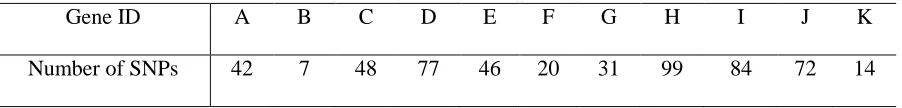
Table 3.1 Gene information for Simulation I. ... 73
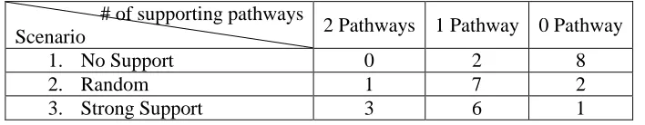
Table 3.2 The biological supports under four scenarios. ... 74
Table 3.3 Different level of biological supports considered in Simulation II... 75
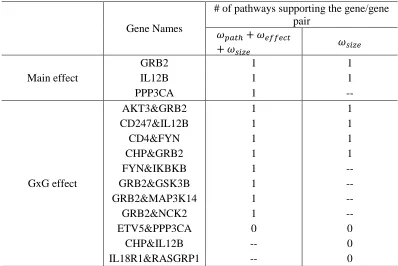
Table 3.4 Real data analysis result ... 76
Table 4.1 Simulation result from Example 1 ... 105
Table 4.2 Simulation result from Example 2 ... 106
Table 4.3 Simulation result from Example 3 ... 107
Table 4.4 Simulation result from Example 4. ... 108
Table 4.5 Simulation result from Example 5. ... 109
Table 4.6 Simulation result from Example 6 ... 110
Table 4.7 Class distribution of the mircoarray data ... 111
Table 4.8 Classification error of the microarray data ... 112
Table 4.9 Real data information. ... 113
LIST OF FIGURES
Figure 2.1 LD pattern of the two genes ... 46
Figure 3.1 Assessment of size weight ... 77
Figure 3.2 Assessment of pathway weight ... 78
Figure 3.3 Assessment of effect weight ... 79
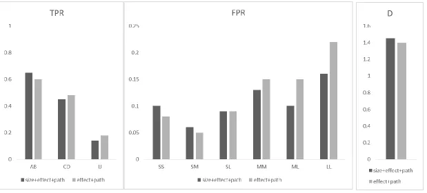
Figure 3.4 Simulation II: quantitative phenotypes ... 80
Figure 3.5 Simulation II: binary phenotype ... 81
Figure 4.1 Data distribution of example 1 ... 115
Figure 4.2 Data distribution of example 2. ... 116
Figure 4.3 Data distribution of example 3 ... 117
Figure 4.4 Data distribution of example 4 ... 118
Figure 4.5 Data distribution of example 5 ... 119
Chapter 1 Introduction
Definition of Gene-Gene interaction (GxG) and its importance
There has been a long-standing interest in the investigation of interactions in genetics, including gene-environment and gene-gene interactions, based on the assumption that they play an important role in the etiology of complex diseases or traits. Biological interaction means physical interaction among biomolecules in gene regulatory networks and biochemical pathways. GxG makes the effect of a gene on a phenotype be dependent on one or more other genes (Bateson, 1909; Moore and Williams, 2005). From the statistical view, interaction means deviation from additivity in a linear model that describes the relationship between multilocus genotype and phenotype variation at the population level (Fisher, 1918). Although there were debates about the relationship between biological interaction and statistical interactions, evidences showed that statistical interactions and biological interactions can converge to the same scientific process (Bush et al., 2009). For example, Bridge used statistical model to identify genes with interaction effects on Drosophila eye color (Bridge, 1919), and the corresponding biological mechanism that depicts how these genes influence biological pathways was understood many years later (Lloyd et al., 1998). Thus, the statistical interaction evidences can be used to infer the biological interactions.
Understanding GxG may also help to uncover the missing heritability (Marchini et al., 2005; Evans et al., 2006) and explain the inconsistent findings from main-effect analyses (Hirschohorn et al., 2002). Even if GxG explains only a tiny fraction of “missing heritability”, the importance of revealing the specific interactions that underlie that fraction would also give us the unique type of biological insight. From such insight, we can having a better understanding of biological mechanisms on both gene level and pathway level.
Current methods for GxG detections
Many methods have been proposed for GxG detection. They can be divided into 2 groups according to whether they consider the interaction at the SNP level or gene level. SNP-based GxG method.
An SNP set may contain just 2 SNPs or all available SNPs. One potential disadvantage of logic regression is that it needs to try all possible SNP combinations and this can be time consuming. Similarly, multivariate adaptive regression splines (MARS) (Friedman 1991; Cook et al., 2004) uses SNP set indicator to represent SNP information rather than using the genotype values of 0, 1, and 2. MARS can also select variables so it is more efficient to find the important GxG. Lin et al. (2008) showed that MARS has a better performance in finding GxG than traditional logistic regression.
Besides the regression models, recursive partitioning approaches are also used to detect GxG interaction by building classification trees. For example, Breiman et al. (1984) proposed classification and regression tree (CART) to find the important genes for the trait. Each SNP can be used as a node in the classification tree to split the population. Important SNPs are first selected and set (?) as parental nodes since they have better abilities to differentiate the observations. Less important SNPs are selected later and set (?) as child nodes to further grow the tree. The tree stops growing until all SNPs are used. The importance of each SNP is measured through the process of tree building.
Many other data-mining approaches have been proposed for mapping GxG interactions, such as genetic programming (Nunkesser et al., 2007), neural networks (Motsinger et al., 2006; Motsinger et al., 2008), pattern-mining (Li et al., 2007; Long et al., 2009), and multifactor dimensionality reduction (MDR) (Ritchie et al., 2001; Hahn et al., 2003; Moore, 2004). MDR was first proposed for case-control data, but later it was extend to quantitative data and adjustment for covariates (Lee et al., 2007; Lou et al., 2007). Similar to random forest, MDR also consider small SNP subsets to find the GxG pattern. Each SNP subset has a pre-specified set size, e.g., each subset contain n SNPs. MDR classifies the genotype combinations of each
n-SNP subset into “high risk” and “low risk” by the ratio of case number and control number under the corresponding genotype combination. An n-SNP set may have many possible genotype combinations but MDR reduce them into 2 possible value. Cross validation is then used to find the best SNP subset with the minimum classification error. MDR has been used to identify GxG in many complex disease, such as breast cancer (Ritchie et al., 2001), type 2 diabetes (Cho et al., 2004), rheumatoid arthritis (Julia et al., 2007) and coronary artery disease (Tsai et al., 2007).
Gene-based GxG method
Hence the gene-level results can be more biologically insightful, easier to interpret, more informative in revealing underlying mechanisms. Second, most genetic variants have different allele frequencies, LD structure, and heterogeneity across diverse human populations while the gene itself is highly consistent across populations. Thus, gene-based method may lead to more consistent results across different studies. Third, modeling the multi-SNPs information within a gene also incorporates the LD among SNPs in the downstreaming analysis. Forth, the polygenic nature of the complex diseases suggests moderate effect size for individual variants. SNPs in aggregate tend to result in more detectable main effects due to the amplification of individual moderate effects Finally, via appropriate dimension reduction to summarize the multi-SNP information, gene-level GxG methods are able to use less degrees of freedom, which further help to gain power improvement over the SNP-level analyses.
component from Principle Component analysis (PCA) to summarize genetic information so that the LDof SNPs within a gene is taken into account. The other way is to use the 1st lead component from Partial Least Square (PLS) analysis to summarize gene information so that not only the LD information but also the correlations between gene and trait are considered. From the simulation study, the PCA or PLS based method have a better performance than the Tukey’s 1-df method, especially when the causal SNP has no or little marginal effect.
GxG detection for large gene set
unimportant genes (Richie, 2011). In current practice, the GxG search space is reduced either in a trait-supervised fashion or using prior biological information.
A widely used trait-supervised method for reducing the search space is the 2-stage method (screen and clean). For the screen step, it would first apply main-effect association tests on each gene|SNP to remove unimportant ones and then model interactions among the remaining ones (Wu et al., 2010). Two interaction mechanisms for Ayotrophic Lateral Sclerosis (ALS) have been identified by such method (Sha et al., 2009). However, filtering out genes/SNPs through main-effect screening would have low power if the casual genes only have strong interaction effect but no main effect.
Recently, some improvements have been made for the 2-stage approach. Boolean Operation-based Screening and Testing (BOOST) and its modified version GBOOST (Wan et al., 2010; Yung et al., 2011) first examines all two-locus interactions in the screening step where promising SNP pairs are determined through a Kulback–Leibler divergence screen. In the following testing stage, likelihood ratio and 𝜒2 tests are performed to check if an interactive
effect is significant.
him/her. Note that the two individuals in one pair may have totally different outcomes, e.g., control vs. case. If a gene is important to the trait, sharing the same genotype would make the paired individuals have no or little trait difference and vice versa. Reliefs sums up all the weighted trait differences to test whether one gene is important to the trait.
Two-stage RF-MARS (TRM) uses RF to screen for important genes and MARS to test the GxG significance. An advantage of TRM is that both RF and MARS automatically select the suitable model based on the data, this feature makes the interaction search more effectively and efficiently.
Instead of directly detecting the significant important GxG, Biofilter (Bush et al., 2009) builds the list of potential important genes based on database such as KEGG, Protein interaction database (PID), Biocarter etc. Its underlying rationale is that if more biological evidences exist to support the interactions among a group of genes, the corresponding statistical evidence for GxG is more credible. Biofilter uses an implication index, which is the number of databases supporting certain GxG, to quantify the strength of biological support. If no databases provide support to certain GxG, it would be removed from the search space. Recent studies (Pendergrass et al., 2013; Turner et al., 2011; Bush et al., 2011) showed that Biofilter can effectively reduce the GxG search space and result in biologically meaningful GxG findings. However, directly filtering out genes without incorporating trait information can be too arbitrary. It is not trait-specific and may limit the chance of finding novel GxG.
There are several advantages to perform statistical analyses coupled with biological guidance. It leads to credible findings with both biological and statistical supports. The results may have higher chances to shed insights in forming follow-up biological hypotheses for further cellular and molecular studies.
Multiclass soft classification using Support vector machine
of tumors, it is usually critical to divide them into several subgroups based on their histopathological type, grade, stage, and genetic information. The knowledge of a specific subtype helps to tailor the treatment approaches and dose levels for increased efficacy and drug sensitivity, low toxicity, and the best outcome. Generally speaking, it’s a multiclass classification problem.
Depending on what the ultimate goal is, classification can be generally divided into hard classification and soft classification. In hard classification, one is only interested in estimating a classification rule (or classifier) which shall be used to assign a label to a new input vector. Popular examples of hard classifiers include support vector machines, nearest neighbor classifiers, and classification trees. On the other hand, the goal of soft classification is to estimate the conditional probabilities of the response belonging to different subclasses. The probability functions are usually more complex than the classification boundary, so in some sense soft classification aims to solve a more difficult problem than hard classification. However, the probability estimates from soft classification provide valuable measure of uncertainty in classification and hence more informative for decision makings.
The traditional SVMs have shown high classification accuracy for many applications in assorted scientific areas such as cancer diagnosis, handwritten digits recognition, junk email detection. However, it does not directly featured with soft classification.
Recently, some methods have been proposed to use SVM to estimate the probabilities for multi-class problem. Wang et al. (2008) demonstrated that soft classification can be achieved by training a series of weighted SVM and then aggregating decision rules to form conditional class probabilities. Wu et al. (2010) generalized this method from the binary case to the multiclass case by training weighted multiclass classifiers. However, the number of weighted multi-category classifiers to be trained increases exponentially fast when the number of classes gets larger or the weight grid becomes finer. The computational cost increases dramatically with the number of classes. In addition, when the overall classification problem changes by adding another class, the results for the original problem cannot be used any more and one needs to start over by training all weighted hard classifiers.
Topic Addressed in this dissertation.
in most cases, the proposed method has a better performance than the other methods. Although in the real data analysis the GxG between the two candidate genes is not significant, one candidate gene is found to be significant important using the conditional main effect test.
In Chapter 3, I give a comprehensive description of how to find GxG among a large number of candidate genes. I use a new penalized L1 regression model that incorporates both biological information and supervision from traits. Specifically, I first apply the principal component (PC) analysis to summarize the multi-SNP genotypes and SNPxSNP design matrix at gene level, and perform gene selections for important main and interaction effects using L1 penalty regression model. The penalty incorporates supports from known pathways related to the trait and trait-supervised adaptive weights. Simulations and real data analysis are used to demonstrate the utility of the pathway-guided penalized regression for GxG identification.
References
Agresti, A. and Coull, B. A. (1998). Approximate is better than 'exact' for interval estimation of binomial proportions. The American Statistician, 52 119-126.
Bateson W. Mendel's Principles of Heredity. Cambridge University Press, Cambridge, UK (1909).
Breiman L, Freidman JH, Olshen RA, Stone CJ. Classification and regression trees. Chapman and Hall/CRC; New York: 1984
Cho YM, Ritchie MD, Moore JH, Park JY, Lee KU, Shin HD, Lee HK, Park KS. Multifactor-dimensionality reduction shows a two-locus interaction associated with Type 2 diabetes mellitus. Diabetologia. 2004;47:549–554.
Combarros, O., et al. Epistasis in sporadic Alzheimer's disease. Neurobiology of Aging, e-publication ahead of print (2008)
Corder, E. H., et al. Gene dose of apolipoprotein E type 4 allele and the risk of Alzheimer's disease in late onset families. Science 261, 921–923 (1993)
Cook NR, Zee RY, Ridker PM (2004) Tree and spline based association analysis of gene–gene interaction models for ischemic stroke. Stat Med 23:1439–1453
Cox, N. J., et al. Loci on chromosomes 2 (NIDDM1) and 15 interact to increase susceptibility to diabetes in Mexican Americans. Nature Genetics 21, 213–215 (1999)
Fisher RA. The correlation between relatives on the supposition of Mendelian inheritance. Trans. R. Soc. Edinb. 52, 399–433 (1918)
Florez, J. C., et al. The inherited basis of diabetes mellitus: Implications for the genetic analysis of complex traits. Annual Review of Genomics and Human Genetics 4, 257–291 (2003). Friedman JH (1991) Multivariate adaptive regression splines. Ann Stat 19:1–66
Hahn LW, Ritchie MD, Moore JH. Multifactor dimensionality reduction software for detecting gene-gene and gene-environment interactions. Bioinformatics. 2003;19:376–382.
Julia A, Moore J, Miquel L, Alegre C, Barcelo P, Ritchie M, Marsal S. Identification of a two-loci epistatic interaction associated with susceptibility to rheumatoid arthritis through reverse engineering and multifactor dimensionality reduction. Genomics. 2007;90:6–13.
Kam-Thong T, Czamara D, Tsuda K, Borgwardt K, Lewis CM, Erhardt-Lehmann A, Hemmer B, Rieckmann P, Daake M, Weber F, et al. EPIBLASTER-fast exhaustive two-locus epistasis detection strategy using graphical processing units. Eur. J. Hum. Genet. 2011;19:465–471. Lee SY, Chung Y, Elston RC, Kim Y, Park T. Log-linear model based multifactor-dimensionality reduction method to detect gene-gene interactions. Bioinformatics. 2007;23:2589–2595. [PubMed]
Li Z, Zheng T, Califano A, Floratos A.. Pattern-based mining strategy to detect multi-locus association and gene environment interaction. BMC Proceedings. 2007
Lin HY, Wang W, Liu YH, Soong SJ, York TP, Myers L, Hu JJ. Comparison of multivariate adaptive regression splines and logistic regression in detecting SNP-SNP interactions and their application in prostate cancer. J Hum Genet. 2008;53(9):802-11.
Long Q, Zhang Q, Ott J. Detecting disease-associated genotype patterns. BMC Bioinformatics. 2009;10
Lou XY, Chen GB, Yan L, Ma JZ, Zhu J, Elston RC, D LM. A generalized combinatorial approach for detecting gene-by-gene and gene-by-environment interactions with application to nicotine dependence. Am J Hum Genet. 2007;80:1125–1137.
Moore JH, Williams SM. Traversing the conceptual divide between biological and statistical epistasis: systems biology and a more modern synthesis. Bioessays. 2005 Jun;27(6):637-46. Moore JH. Computational analysis of gene-gene interactions using multifactor dimensionality reduction. Expert Rev Mol Diagn. 2004;4:795–803.
Motsinger A, Lee S, Mellick G, Ritchie M. GPNN: power studies and applications of a neural network method for detecting gene-gene interactions in studies of human disease. BMC Bioinformatics. 2006;7:39.
Nunkesser R, Bernholt T, Schwender H, Ickstadt K, Wegener I. Detecting high-order interactions of single nucleotide polymorphisms using genetic programming. Bioinformatics. 2007;23:3280–3288.
Ritchie MD, Hahn LW, Roodi N, Bailey LR, Dupont WD, Parl FF, Moore JH. Multifactor-dimensionality reduction reveals high-order interactions among estrogen-metabolism genes in sporadic breast cancer. Am J Hum Genet. 2001;69:138–147.
Saunders, A. M., et al. Association of apolipoprotein E allele epsilon 4 with late-onset familial and sporadic Alzheimer's disease. Neurology 43, 1467–1472 (1993)
Schupbach T, Xenarios I, Bergmann S, Kapur K. FastEpistasis: a high performance computing solution for quantitative trait epistasis. Bioinformatics. 2010;26:1468–1469.
Strittmatter, W. J., et al. Apolipoprotein E: High-avidity binding to beta-amyloid and increased frequency of type 4 allele in late-onset familial Alzheimer disease. Proceedings of the National Academy of Sciences 90, 1977–1981 (1993).
Tsai CT, Hwang JJ, Ritchie MD, Moore JH, Chiang FT, Lai LP, Hsu KL, Tseng CD, Lin JL, Tseng YZ. Renin-angiotensin system gene polymorphisms and coronary artery disease in a large angiographic cohort: detection of high order gene-gene interaction. Atherosclerosis. 2007;195:172–180.
Wan X, Yang C, Yang Q, Xue H, Fan X, Tang NLS, Yu W. BOOST: a fast approach to detecting gene-gene interactions in genome-wide case-control studies. Am.J. Hum. Genet. 2010;87:325–340.
Wang, J., Shen, X. and Liu, Y. (2008). Probability estimation for large margin classifiers. Biometrika, 95 149-167.
Wiltshire, S., et al. Epistasis between type 2 diabetes susceptibility loci on chromosomes 1q21– 25 and 10q23–26 in northern Europeans. Annals of Human Genetics 70, 726–737 (2006) Wu, Y., Zhang, H. H. and Liu, Y. (2010). Robust model-free multiclass probability estimation. Journal of the American Statistical Association., 105 424-436.
Zhang Y, Liu JS. Bayesian inference of epistatic interactions in case-control studies. Nat Genet. 2007;39:1167–1173.
Chapter 2
Gene-Gene Interactions Using Gene-Trait Similarity Regression
Introduction
Gene-Gene Interactions (GxG) are believed to be ubiquitous in biology system (Moore, 2003; Carlborg and Haley, 2004) and to play an important role in gene regulation, signal transduction, biochemical networks, and many other physiological and developmental pathways (Moore, 2003; Greenspan, 2001; Phenix et al., 2013; Barkoulas et al., 2013). Identifying GxG may improve the ability to find the susceptible genes and provide insights into biological mechanisms for complex disease, such as Alzheimer’s disease, diabetes, cardiovascular and cancer (Lin et al., 2013; Pillai et al., 2013; Koh-Tan et al., 2013; Howson et al., 2012; Ziyab et al., 2013). It may also help to explain the missing heritability and the inconsistent findings in many genetic association studies (Marchini et al., 2005; Evans et al., 2006).
Sham, 2004; Wang et al., 2009). First,genes are the basic units in the biological mechanism and SNPs within a gene tend to work concordantly. Thus gene-level results may be more biologically insightful, easier to interpret or more informative in revealing underlying mechanisms. Second, the correlations between SNPs are considered when modeling multi-SNP information. Third, multi-SNPs in aggregate tend to result in more detectable main effects due to the amplification of individual moderate effects. We expect a similar amplification effect to exist for GxG effects. Finally, because gene-level GxG methods tend to use less degree of freedom, it is expected to gain potential more power than SNP level analysis.
traits are considered. From the simulation study, the PCA or PLS based method have a better performance than the Tukey’s 1-df method, especially when the causal SNP has no or little marginal effect.
Here we propose a new method using the gene-trait similarity regression (SimReg) to detect GxG at gene level. This regression model correlates trait similarity with gene level genetic similarity. Compare to the PCA/PLS based methods, the proposed method provide the following improvement. First, PCA/PLS tend to suffer from information lose in the dimension reduction process by using only the first component, or encounter curse of dimensionality if multiple components are used. In contrast, SimReg incorporates all SNP information within a gene while performing GxG test with a small degrees of freedom. Second, first component from PCA or PLS is actually a sum of weighted SNP genotypes. The interaction term formed by multiplying the two linear combinations would only capture limited forms of non-additive effect. In contrast, as we describe in the method section, SimReg is capable to model a variety of effects by selecting different metrics to quantify gene similarity. Finally, the GxG test under the SimReg framework is computationally efficient because the permutations are not required.
present the simulation study (Section 3) and a real data application on the warfarin study of Wysowski et al. (2007) (Section 4). Finally, we discuss the limitations and future research directions.
Method
The Gene-Trait Similarity Model
Denote 𝑌𝑖 as the trait value, 𝑋𝑖 the 𝐾 × 1 covariant vector including the intercept term, and 1 × 𝑙𝑚 vector 𝐺𝑚,𝑖 records genotypes at marker 𝑚 for 𝑖th individual. Define 𝑆𝑖𝑗𝐴 to be the
genetic similarity of gene A between subjects 𝑖 and 𝑗 (𝑖 ≠ 𝑗). There are many ways to describe the genetic similarity between individuals. Here, we consider the weighted IBS sum across the 𝑀𝐴 loci in gene A, i.e., for subjects 𝑖 and 𝑗, the similarity level is 𝑆𝑖𝑗𝐴 = ∑𝑀𝐴
𝑚=1𝑤𝑚𝑠𝑚,𝑖𝑗 where
𝑠𝑚,𝑖𝑗 = 𝑥/2 if 𝐺𝑚,𝑖 and 𝐺𝑚,𝑗 have 𝑥 alleles in common. The similarity level in gene B, 𝑆𝑖𝑗𝐵, can
be defined in the same manner. The trait similarity between individual 𝑖 and 𝑗, denoted by 𝑍𝑖𝑗, is computed by
𝑍𝑖𝑗 = (𝑌𝑖 − 𝜇𝑖)(𝑌𝑗− 𝜇𝑗),
where 𝜇𝑖 = 𝐸(𝑌𝑖|𝑋𝑖, 𝐺𝑖) = 𝑋𝑖𝛾, which is the conditional trait mean given covariate
information but assuming no genotype effect and 𝛾 is the effect of the covariates. The gene-trait similarity regression for gene-gene interactions is given as
𝐸(𝑍𝑖𝑗|𝑋, 𝐺) = 𝜏𝐴𝑆𝑖𝑗𝐴+ 𝜏
In Model (1), we use the product of the similarity scores, 𝑆𝑖𝑗𝐴𝑆𝑖𝑗𝐵, to model the GxG effect. Note that the regression model has zero intercept because the covariates have been incorporated when quantifying trait similarity (Tzeng et al., 2009).
The Interaction Test
The interaction test examines the hypothesis 𝐻0,𝐼𝑛𝑡: 𝜏𝐴𝐵 = 0. Direct derivation of a test statistic under Model (1) can be burdensome because Model (1) is a regression whose observation unit is pairs of individuals. Consequently, the observations are correlated when two pairs share a common individual. The variance-covariance matrix for 𝑍 is a non-sparse matrix with dimension ( )𝑛2 by ( )
2
𝑛 , which is computationally challenging to inverse so to obtain
the test statistics. To bypass these issues, we derive the score test based on the equivalence between the similarity regression and a mixed effect model (Tzeng et al., 2009; Tzeng et al., 2011). To see this, consider the following working mixed model:
𝑌𝑖 = 𝑋𝑖𝛾 + 𝑔𝐴,𝑖+ 𝑔𝐵,𝑖+ 𝑔𝐴𝐵,𝑖 + 𝑒𝑖, (2)
where 𝑒𝑖 ∼ 𝑁(0, 𝜎), and 𝑔𝐴,𝑖, 𝑔𝐵,𝑖 and 𝑔𝐴𝐵,𝑖 are subject-specific genetic effects for gene A, gene B and interaction between genes A and B, respectively. Let 𝑔𝐴T = [𝑔
𝐴,1, ⋯ , 𝑔𝐴,𝑛],
𝑔𝐵T = [𝑔
𝐵,1, ⋯ , 𝑔𝐵,𝑛], and 𝑔𝐴𝐵T = [𝑔𝐴𝐵,1, ⋯ , 𝑔𝐴𝐵,𝑛], and assume that
𝑔𝐴 ∼ 𝑀𝑁(0, 𝑣𝐴𝑆𝐴), 𝑔𝐵 ∼ 𝑀𝑁(0, 𝑣𝐵𝑆𝐵), 𝑔𝐴𝐵 ∼ 𝑀𝑁(0, 𝑣𝐴𝐵𝑆𝐴𝐵),
where matrix 𝑆𝐴 = {𝑆𝑖𝑗𝐴}
𝑛×𝑛, 𝑆𝐵 = {𝑆𝑖𝑗 𝐵}
𝑛×𝑛, and 𝑆𝐴𝐵 = {𝑆𝑖𝑗 𝐴× 𝑆
𝑖𝑗𝐵}𝑛×𝑛. In other words,
is governed by the genetic similarity between the two individuals in gene A (𝑆𝑖𝑗𝐴). Then the marginal trait covariance in Model (2) can be obtained by
𝑐𝑜𝑣(𝑌𝑖, 𝑌𝑗|𝑋, 𝐺) = 𝑐𝑜𝑣𝑔⋅{𝐸(𝑌𝑖|𝑿, 𝐺, 𝑔𝐴, 𝑔𝐵, 𝑔𝐴𝐵), 𝐸(𝑌𝑖|𝑿, 𝐺, 𝑔𝐴, 𝑔𝐵, 𝑔𝐴𝐵)} (3) = 𝑐𝑜𝑣𝑔⋅{𝑋𝑖𝛾 + 𝑔𝐴,𝑖+ 𝑔𝐵,𝑖+ 𝑔𝐴𝐵,𝑖, 𝑋𝑗𝛾 + 𝑔𝐴,𝑗 + 𝑔𝐵,𝑗+ 𝑔𝐴𝐵,𝑗}
= 𝑣𝐴𝑆𝑖𝑗𝐴+ 𝑣
𝐵𝑆𝑖𝑗𝐵+ 𝑣𝐴𝐵𝑆𝑖𝑗𝐴𝑆𝑖𝑗𝐵.
Comparing (3) with (1), we have 𝜏𝐴 = 𝑣𝐴, 𝜏𝐵 = 𝑣𝐵, and 𝜏𝐴𝐵 = 𝑣𝐴𝐵. That is, the regression coefficients in the similarity regression model are variance components in the working linear mixed effect model.
We derive the score function of the REML log-likelihood function of Model (2) in Appendix A, and obtain the score statistic under 𝐻0,𝐼𝑛𝑡 as
𝑇𝐼𝑛𝑡 = 12𝒀′𝑃
𝐼𝑛𝑡𝑆𝐴𝐵𝑃𝐼𝑛𝑡𝒀|𝜏
𝐴=𝜏̂𝐴,𝜏𝐵=𝜏̂𝐵,𝜎=𝜎̂ ,
where the trait value 𝒀T = (𝑌1, . . . , 𝑌𝑛), 𝑿 = (𝑋1; 𝑋2; ⋯ ; 𝑋𝑛) 𝑃𝐼𝑛𝑡 = 𝑉𝐼𝑛𝑡−1− 𝑉𝐼𝑛𝑡−1𝑿(𝑿′−1𝑉
𝐼𝑛𝑡−1𝑿)−1𝑿′𝑉𝐼𝑛𝑡−1 , 𝑉𝐼𝑛𝑡 = 𝜏𝐴𝑆𝐴+ 𝜏𝐵𝑆𝐵+ 𝜎𝐼 and (𝜏̂𝐴, 𝜏̂𝐵, 𝜎̂) are the maximum
REML estimates obtained under 𝐻0,𝐼𝑛𝑡: 𝜏𝐴𝐵 = 0. We describe an adaptive EM algorithm to obtain (𝜏̂𝐴, 𝜏̂𝐵, 𝜎̂) in Appendix B.
Under the alternative hypothesis 𝜏𝐴𝐵 ≠ 0, 𝑇𝐼𝑛𝑡 is a strictly increasing function of 𝜏𝐴𝐵.
Therefore larger values of 𝑇𝐼𝑛𝑡 provides stronger evidence against 𝐻0,𝐼𝑛𝑡. This suggests that
the testing procedure should be one sided. As shown in Appendix A, the distribution of 𝑇𝐼𝑛𝑡 follows a weighted 𝜒2 distribution. That is, define 𝐶
𝑇𝐼𝑛𝑡 has the same distribution as ∑𝑐
𝑗=1 𝜆𝑗,𝐼𝑛𝑡𝜒12 , where 𝜆𝑗,𝐼𝑛𝑡 is the ordered none zero
eigenvalues of matrix 𝐶𝐼𝑛𝑡. The p-values can be calculated using moment-matching approximations (Liu et al., 2009; Duchesne et al., 2010).
The Joint Test
Instead of evaluating the GxG effects between two genes, one may be interested in assessing the overall effect from the two genes, regardless the main effects or interaction effects. To do so, we construct a joint test to examine the null hypothesis of 𝐻0,𝐽𝑜𝑖𝑛𝑡: 𝜏𝐴 =
𝜏𝐵 = 𝜏𝐴𝐵 = 0 under the full model 𝐸(𝑍𝑖𝑗|𝑋, 𝐺) = 𝜏𝐴𝑆𝑖𝑗𝐴+ 𝜏𝐵𝑆𝑖𝑗𝐵+ 𝜏𝐴𝐵𝑆𝑖𝑗𝐴𝑆𝑖𝑗𝐵. As shown in Appendix A, the test statistic is given as
𝑇𝐽𝑜𝑖𝑛𝑡 =12𝒀′𝑃
𝐽𝑜𝑖𝑛𝑡(𝑆𝐴+ 𝑆𝐵+ 𝑆𝐴𝐵)𝑃𝐽𝑜𝑖𝑛𝑡𝒀| 𝜎=𝜎̆,
where 𝑃𝐽𝑜𝑖𝑛𝑡 = 𝜎−1{𝐼 − 𝑿(𝑿′𝑿)−1𝑿′} and 𝜎̆ = 𝒀
′{𝐼−𝑿(𝑿′𝑿)−1𝑿′}𝒀
(𝑛−𝐾) , where 𝐾is number
of covariates. The distribution of 𝑇𝐽𝑜𝑖𝑛𝑡 also follows a weighted 𝜒2 distribution, i.e., 𝑇𝐽𝑜𝑖𝑛𝑡 has
the same distribution as ∑𝑐𝑗=1 𝜆𝑗,𝐽𝑜𝑖𝑛𝑡𝜒12 with 𝜆𝑗,𝐽𝑜𝑖𝑛𝑡 the ordered nonzero eigenvalues of 𝐶𝐽𝑜𝑖𝑛𝑡 =12𝑉𝐽𝑜𝑖𝑛𝑡1/2 𝑃𝐽𝑜𝑖𝑛𝑡(𝑆𝐴+ 𝑆𝐵+ 𝑆𝐴𝐵)𝑃𝐽𝑜𝑖𝑛𝑡𝑉𝐽𝑜𝑖𝑛𝑡1/2 .
The Conditional Main Effect Test
interacting variables. Consider the full model: 𝐸(𝑍𝑖𝑗) = 𝜏𝐴𝑆𝐴,𝑖𝑗+ 𝜏𝐵𝑆𝐵,𝑖𝑗. The effect of Gene
A accounting for the effect of Gene B can be assessed by examining the hypothesis of 𝐻0,𝐴:
𝜏𝐴 = 0. Similar to previous two tests, the score test statistic for gene A is given as: 𝑇𝐴 = 12𝒀′𝑃
𝐴𝑆𝐴𝑃𝐴𝒀|
𝜏𝐵=𝜏̃𝐵,𝜎=𝜎̃ ,
where 𝑃𝐴 = 𝑉𝐴−1− 𝑉𝐴−1𝑿(𝑿′−1𝑉𝐴−1𝑿)−1𝑿′𝑉𝐴−1, 𝑉𝐴 = 𝜏𝐵𝑆𝐵+ 𝜎𝐼, and (𝜏̃𝐵, 𝜎̃) are the maximum REML estimates obtained under 𝐻0,𝐴: 𝜏𝐴 = 0. We describe the adaptive EM
algorithms to obtain (𝜏̃𝐵, 𝜎̃) in Appendix B. As shown in Appendix A, 𝑇𝐴 has the same distribution as ∑𝑐𝑗=1 𝜆𝑗,𝐴𝜒12 with 𝜆𝑗,𝐴 the ordered nonzero eigenvalues of 𝐶𝐴 =
1 2𝑉𝐴
1/2𝑃
𝐴𝑆𝐴𝑃𝐴𝑉𝐴1/2. The test statistic for assessing the conditional main effect of gene B, 𝑇𝐵,
can be defined similarly. Simulation study
Design for Simulation Study
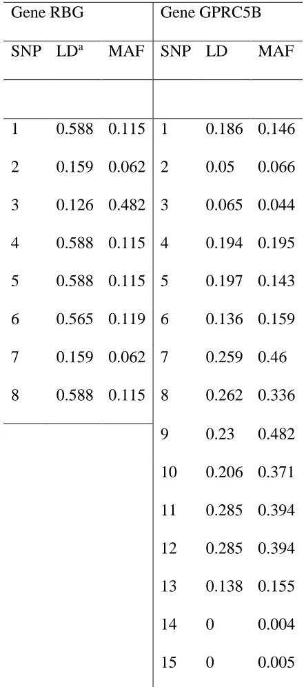
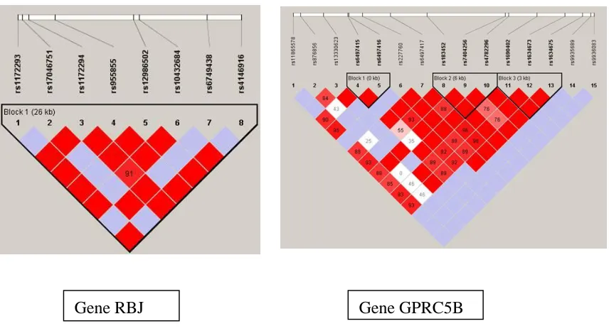
To simulate genotype data with realistic LD patterns, we use genotype data of Gene RBJ (8 SNPs) and Gene GPRC5B (15 SNPs) downloaded from HapMap (http://hapmap.ncbi.nlm.nih.gov/). The LD structure of the two genes are given in Figure 1.
For each SNP in a given gene, we list in Table 2.1 its minor allele frequency (MAF) and LD, which is quantified by the average of 𝑅2 between the target SNP and the remaining
SNPs in the same gene. We considered two causal SNPs from each gene and simulate the trait values based on the model:
𝑌 = 𝛽𝐴× (𝑆𝑁𝑃1𝐴+ 𝑆𝑁𝑃2𝐴+ 𝑆𝑁𝑃1𝐴× 𝑆𝑁𝑃2𝐴)
+𝛽𝐵× (𝑆𝑁𝑃1𝐵+ 𝑆𝑁𝑃
2𝐵+ 𝑆𝑁𝑃1𝐵× 𝑆𝑁𝑃2𝐵)
+𝛽𝐴𝐵× (𝑆𝑁𝑃1𝐴× 𝑆𝑁𝑃
1𝐵+ 𝑆𝑁𝑃2𝐴× 𝑆𝑁𝑃2𝐵) + 𝑒, (4)
where 𝑆𝑁𝑃1𝐴 and 𝑆𝑁𝑃
2𝐴 are the number of the minor alleles carried by a subject at the
first and second causal loci in Gene A; 𝑆𝑁𝑃1𝐵 and 𝑆𝑁𝑃
2𝐵 are defined similarity; 𝑒 follows a
normal distributed variable with mean 0 and variance 1. The trait value 𝑌 depended on three components: the gene effect from Gene A, the gene effect from Gene B and the interaction effect between Gene A and Gene B. There is no LD between RBJ and GPRC5B because the genotypes of a person for the two genes were sampled independently.
0); (3) both Gene A and Gene B have main effect to the trait (𝛽𝐴 ≠ 0, 𝛽𝐵≠ 0, 𝛽𝐴𝐵 = 0). For the conditional main effect (𝐻0: 𝜏𝐵 = 0), we consider two scenarios of no gene B effect: (1) both gene have no genetic effect (𝛽𝐴 = 𝛽𝐵= 𝛽𝐴𝐵 = 0); (2) Gene A has a main effect to the trait (𝛽𝐴 ≠ 0, 𝛽𝐵 = 0, 𝛽𝐴𝐵 = 0). For each scenario, we ran the simulation for 1,000 replications
and each replication consisted of 300 subjects to compute the type I error rates.
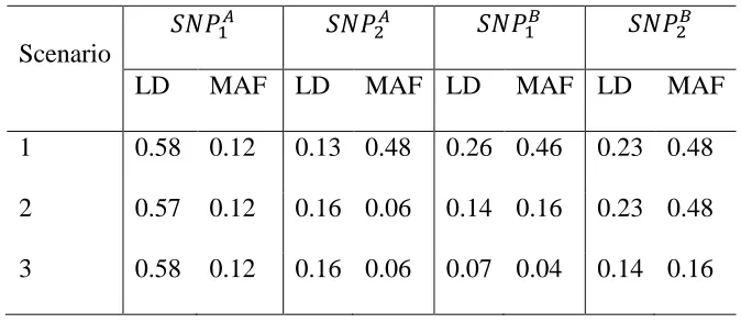
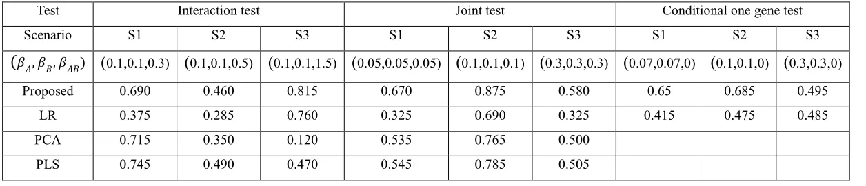
For power analysis, we considered three different scenarios based on the genetic architecture of the causal SNPs. Specifically, we selected three SNP pairs with certain LD and MAF as causal SNPs (Table 2.2). When generating trait values using the Model (4), we considered different 𝛽 values so that power of different methods are between 20%~80%. Simulation result
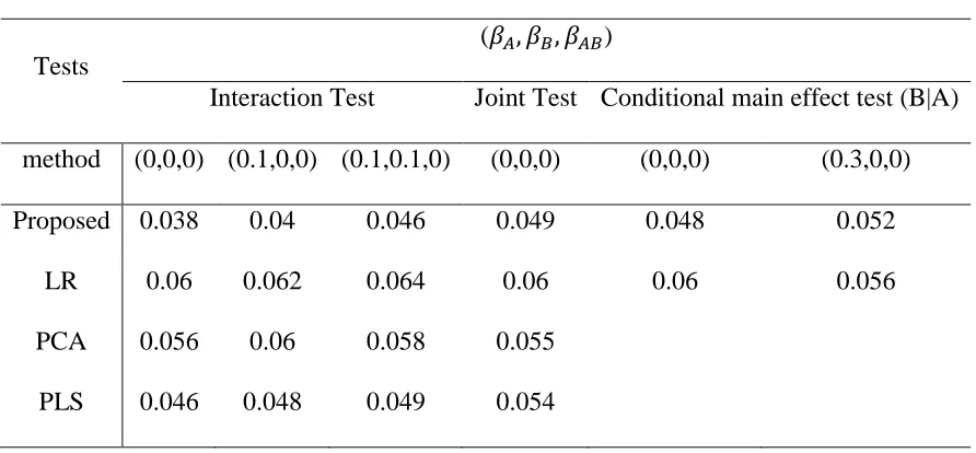
Table 2.3 shows the type I error rates for different methods at a significance level of 𝛼 = 0.05. The type I error rates of all approaches are around the nominal level in all different
settings except in some scenarios for interaction test. The type I error rates of the proposed interaction tests were conservative when 𝛽𝐴 = 𝛽𝐵 = 0 (and hence 𝜏𝐴 = 𝜏𝐵 = 0). As one or both of 𝜏𝐴 and 𝜏𝐵 became further away from 0, e.g., 0.1, the type I error rates get better. As
For joint test, we see that proposed method always gain the best power, followed by PLS and PCA. PLS and PCA performed similarly but PLS always had a better power than PCA. The observation is consistent with Wang et al. (2009) since first component from PLS considers both LD and correlation between trait and gene information. All the three methods performed better than LR, as it may lose power due to large degree of freedoms. In joint test, the proposed method had the best performance while in interaction test, PLS/PCA may had better power gain in some scenarios. Possible reason is that the proposed approach needs to estimate nuisance under the 𝐻0 in the interaction test. The corresponding EM estimates can be biased when the true values are 0 or close to 0. This may lead to too conservative results and cause power loss.
For conditional main effect test, proposed method always has a better power than linear model, but the difference between proposed method and linear model gets smaller as the LD and MAF of causal SNP is smaller. The finding is consistent with the finding in the interaction test: LR has a robust performance against LD and MAF.
Real Data Analysis
consequence such as bleeding, swelling of face, throat. Extensive researches have been conducted to develop method for predicting the appropriate dose.
We have conducted a genetic analysis using the data from the Warfarin study (The International Warfarin Pharmacogenetics Consortium, 2009). In this data set, 2 genes are involved, gene VKORC1 contains 7 SNPs and gene CYP2C9 is a tri-allelic locus. After quality control, this data set involves 301 individuals and records their stable warfarin dose. Also available are 4 detected covariates associated with warfarin therapy: age, sex, height and weight for each individuals in the study.
We apply the proposed method and the benchmark methods to detect the association between the warfarin dose and the genes. The results are summarized in Table 2.5. All methods identify significant association between trait and the two genes. But the proposed method exhibits the strongest evidence of association among all the approaches, which is consistent with the simulation results that the proposed method is more powerful than other methods. These results also suggest that there are no interactions between the two genes, and Gene VKORC1 has more significant impact on the warfarin dose.
Discussion
of the underlying mechanisms for complex diseases. Although the majority of GxG methods focus on SNP-SNP interactions, gene-based GxG methods may hold great promises in biological interpretation and power gain. In this paper, we propose a similarity regression model for studying GxG at gene level. We provide three tests to evaluate the effect of interest: interaction test, joint test and conditional main effect test. The simulation results showed that the proposed method had a consistent satisfactory performance under different genetic architectures. In contrast, PLS, PCA, and LR performed quite differently depending the LD and MAF of the causal SNPs.
In the proposed model, we used an adaptive EM algorithm to estimate the nuisance parameters 𝜏𝐴 and 𝜏𝐵. Directly applying the traditional EM algorithm without any adjustment
may lead to sizable biases and is time-consuming for converge when the true values of 𝜏𝐴 and
𝜏𝐵 were zero. The adaptive EM algorithm reduces the bias and computational time, and improves the type I rates although they are still conservative when true 𝜏𝐴 and 𝜏𝐵 equal to 0. How to improve the variance estimation when the true value is at the zero boundary would be an interesting topic for further research.
applying a LD analysis first, then splitting the large gene into several smaller blocks to do the GxG interaction detection.
Appendix A. Derivation of the score tests and their distributions Consider the matrix presentation of model (2):
𝐘 = 𝐗𝛾 + 𝑔𝐴+ 𝑔𝐵+ 𝑔𝐴𝐵+ 𝑒.
The corresponding REML log-likelihood function, denoted as 𝐿(𝜏𝐴, 𝜏𝐵, 𝜏𝐴𝐵, 𝜎), is: 𝐿(𝜃) = −12[log|𝑉| + log|𝐗′−1𝑉𝐗| + 𝐘′𝑃𝐘],
where 𝑉 = 𝑉𝑎𝑟(𝑌) = 𝜏𝐴𝑆𝐴+ 𝜏𝐵𝑆𝐵+ 𝜏𝐴𝐵𝑆𝐴𝐵+ 𝜎𝐼 is the marginal variance of 𝐘 and 𝑃 = 𝑉−1− 𝑉−1𝐗(𝐗′−1𝑉−1𝐗)−1𝐗′𝑉−1 is the projection matrix for the model. The score
functions of 𝜏𝐴, 𝜏𝐵, and 𝜏𝐴𝐵 based on 𝐿(𝜃) are
𝑈𝜏𝐴(𝜏𝐴, 𝜏𝐵, 𝜏𝐴𝐵, 𝜎) =∂𝐿(𝜏𝐴,𝜏∂𝜏𝐵,𝜏𝐴𝐵,𝜎)
𝐴 =
1
2[𝐘′𝑃𝑆𝐴𝑃𝐘 − 𝑡𝑟(𝑃𝑆𝐴)],
𝑈𝜏𝐵(𝜏𝐴, 𝜏𝐵, 𝜏𝐴𝐵, 𝜎) =∂𝐿(𝜏𝐴,𝜏∂𝜏𝐵,𝜏𝐴𝐵,𝜎)
𝐵 =
1
2[𝐘′𝑃𝑆𝐵𝑃𝐘 − 𝑡𝑟(𝑃𝑆𝐵)], and
𝑈𝜏𝐴𝐵(𝜏𝐴, 𝜏𝐵, 𝜏𝐴𝐵, 𝜎) =∂𝐿(𝜏𝐴,𝜏𝐵,𝜏𝐴𝐵,𝜎) ∂𝜏𝐴𝐵 = 1 2[𝐘 ′𝑃𝑆 𝐴𝐵𝑃𝐘 − 𝑡𝑟(𝑃𝑆𝐴𝐵)].
We construct the statistics based on the first terms of the score functions. Here after we define matrices 𝑃ℎ and 𝑉ℎ as 𝑃 and 𝑉 evaluated under 𝐻0,ℎ. Then for the interaction test 𝐻0,𝐼𝑛𝑡: 𝜏𝐴𝐵 = 0, we set the test statistic as
𝑇𝐼𝑛𝑡 = 12𝐘′𝑃𝐼𝑛𝑡𝑆𝐴𝐵𝑃𝐼𝑛𝑡𝐘|
𝜏𝐴=𝜏̂𝐴,𝜏𝐵=𝜏̂𝐵,𝜎=𝜎̂ ,
For the conditional main effect test 𝐻0,𝐴: 𝜏𝐴 = 0 under the constrain of no interaction
(i.e., 𝜏𝐴𝐵 = 0), we set the test statistic as
𝑇𝐴 = 12𝐘′𝑃𝐴𝑆𝐴𝑃𝐴𝐘|
𝜏𝐵=𝜏̃𝐵,𝜎=𝜎̃ ,
where 𝑃𝐴 = 𝑉𝐴−1− 𝑉𝐴−1𝐗(𝐗′−1𝑉𝐴−1𝐗)−1𝐗′𝑉𝐴−1, 𝑉𝐴 = 𝜏𝐵𝑆𝐵+ 𝜎𝐼, and (𝜏̃𝐵, 𝜎̃) are the maximum REML estimates obtained under 𝐻0,𝐴: 𝜏𝐴 = 0 . The test statistic 𝑇𝐵 can be defined similarily for examining 𝐻0,𝐵: 𝜏𝐵 = 0 under the constrain of 𝜏𝐴𝐵 = 0.
We describe the EM algorithms that we use to obtain (𝜏̂𝐴, 𝜏̂𝐵, 𝜎̂) and (𝜏̃𝐵, 𝜎̃) in Appendix B.
For the joint test 𝐻0,𝐽𝑜𝑖𝑛𝑡: 𝜏𝐴 = 𝜏𝐵= 𝜏𝐴𝐵 = 0, because 𝜏's are non-negative variance components, 𝜏𝐴 = 𝜏𝐵 = 𝜏𝐴𝐵 = 0 if and only if 𝜏𝐴+ 𝜏𝐵+ 𝜏𝐴𝐵 = 0. This motivates us to
construct the test statistic based on the sum of the three score functions. That is, 𝑇𝐽𝑜𝑖𝑛𝑡 =12𝐘′𝑃
𝐽𝑜𝑖𝑛𝑡(𝑆𝐴+ 𝑆𝐵+ 𝑆𝐴𝐵)𝑃𝐽𝑜𝑖𝑛𝑡𝐘|𝜎=𝜎̆,
where the 𝑃𝐽𝑜𝑖𝑛𝑡 = 𝑉𝐽𝑜𝑖𝑛𝑡−1 − 𝑉𝐽𝑜𝑖𝑛𝑡−1 𝐗(𝐗′−1𝑉𝐽𝑜𝑖𝑛𝑡−1 𝐗)−1𝐗′𝑉𝐽𝑜𝑖𝑛𝑡−1 , 𝑉𝐽𝑜𝑖𝑛𝑡 = 𝜎𝐼 and 𝜎̆ = 𝐘′{𝐼 − 𝐗(𝐗′𝐗)−1𝐗′}𝐘/(𝑛 − 𝐾).
The distributions of the test statistics can be shown to follow a weighted chi-squared distribution via the fact that these statistics are quadratic form of 𝐘. To illustrate, consider 𝑇𝐼𝑛𝑡 =12𝐘′𝑃
𝐼𝑛𝑡𝑆𝐴𝐵𝑃𝐼𝑛𝑡𝐘. Because 𝑃𝐼𝑛𝑡 is a projection matrix, 𝑃𝐼𝑛𝑡𝐗𝛾 = 0. Therefore,
𝑇𝐼𝑛𝑡 =12𝐘′𝑃𝐼𝑛𝑡𝑆𝐴𝐵𝑃𝐼𝑛𝑡𝐘 = 12(𝐘 − 𝐗𝛾)′𝑃𝐼𝑛𝑡𝑆𝐴𝐵𝑃𝐼𝑛𝑡(𝐘 − 𝐗𝛾) =12(𝐘 −
𝐗𝛾)′𝑉
Define 𝐳 = 𝑉𝐼𝑛𝑡−1/2(𝐘 − 𝐗𝛾) and 𝐶𝐼𝑛𝑡 = 12𝑉𝐼𝑛𝑡1/2𝑃𝐼𝑛𝑡𝑆𝐴𝐵𝑃𝐼𝑛𝑡𝑉𝐼𝑛𝑡1/2, we have 𝑇𝐼𝑛𝑡 = 𝐳′𝐶
𝐼𝑛𝑡𝐳 ~ ∑𝑐𝑗=1 𝜆𝑗,𝐼𝑛𝑡𝜒12, where 𝜆𝑗,𝐼𝑛𝑡 is the ordered none zero eigenvalues of matrix 𝐶𝐼𝑛𝑡. By
the same mannar, one can obtain that 𝑇𝐴 ~ ∑𝑐𝑗=1 𝜆𝑗,𝐴𝜒12 with 𝜆𝑗,𝐴 the ordered nonzero eigenvalues of 𝐶𝐴 =12𝑉𝐴1/2𝑃𝐴𝑆𝐴𝑃𝐴𝑉𝐴1/2, and 𝑇𝐽𝑜𝑖𝑛𝑡 ~ ∑𝑐𝑗=1 𝜆𝑗,𝐽𝑜𝑖𝑛𝑡𝜒12 with 𝜆𝑗,𝐽𝑜𝑖𝑛𝑡 the ordered
nonzero eigenvalues of 𝐶𝐽𝑜𝑖𝑛𝑡 = 12𝑉𝐽𝑜𝑖𝑛𝑡1/2 𝑃𝐽𝑜𝑖𝑛𝑡(𝑆𝐴+ 𝑆𝐵+ 𝑆𝐴𝐵)𝑃𝐽𝑜𝑖𝑛𝑡𝑉𝐽𝑜𝑖𝑛𝑡1/2 .
Appendix B. The adaptive EM algorithm to obtain the maximum REML estimates In interaction test and conditional one gene test, we use EM algorithm to estimate the nuisance parameter under the corresponding 𝐻0. The regular EM algorithm has caused too conservative results since it provides non-negative estimates for the nuisance variance components 𝜏𝐴, 𝜏𝐵 and 𝜎. Thus, when 𝜏𝐴 and/or 𝜏𝐵 are 0 or close to 0, the EME can be biased
as 𝐸( 𝜏̂ ) > 𝜏𝐴 𝐴 and 𝐸(𝜏̂) > 𝜏𝐵 𝐵. This motived us to use and adaptive procedure to address this problem. We first apply conditional main effect tests for 𝐻0: 𝜏𝐴 = 0 and 𝐻0: 𝜏𝐵= 0. If we fail to reject the null hypothesis, the corresponding 𝜏̂ is set to 0. If 𝜏 is significant different from 0, EM algorithm is used to estimate 𝜏. By applying this adaptive EM, 𝐸(𝜏̂) would be closer to 0 when the 𝜏 is 0 or close to 0. When 𝜏 are relative large, the conditional main effect test would reject 𝐻0: 𝜏 = 0 and the estimate from t he adaptive EM is the same as the original EME.
For interaction test, when we do the type I error analysis, we found that the statistics 𝑇𝐼𝑛𝑡 does not fit the estimated weighted 𝜒2 distribution perfectly if the true value of 𝜏
𝐴 and 𝜏𝐵
estimated weighted 𝜒2 well. The main reason for this scenoraio is that the estimated 𝜏 𝐴
̂ and 𝜏̂ are always biased to the true value since EM algorithm could only give us positive estimates 𝐵 for 𝜏̂𝐴 and 𝜏̂𝐵. Thus, it is always true that 𝐸(𝜏̂𝐴) > 𝜏𝐴 and 𝐸(𝜏̂𝐵) > 𝜏𝐵, and the difference between 𝐸(𝜏̂) and 𝜏 would be huge when 𝜏𝐴 are 0 or close to 0.
We first describe the EM algorithm for (𝜏̂𝐴, 𝜏̂𝐵, 𝜎̂), i.e., the maximum REML estimates
under 𝐻0,𝐼𝑛𝑡: 𝜏𝐴𝐵 = 0. Under 𝐻0,𝐼𝑛𝑡, the LMM is
𝐘 = 𝐗𝛾 + 𝑔𝐴+ 𝑔𝐵+ 𝑒,
where 𝑒~𝑁(0, 𝜎𝐼), 𝑔𝐴~𝑁(0, 𝜏𝐴𝑆𝐴) and 𝑔𝐵~𝑁(0, 𝜏𝐵𝑆𝐵) as 𝜏𝐴 = 𝜈𝐴 and 𝜏𝐵= 𝜈𝐵. Define 𝑈 = 𝐴𝑇𝐘 with the restriction that 𝐴𝑇𝐴 = 𝐼𝑛−𝐾 and 𝐴𝐴𝑇 = 𝐼 − 𝐗(𝐗′𝐗)−1𝐗. Then 𝑈|𝑔𝐴, 𝑔𝐵 ~𝑁(𝐴′𝑔𝐴 + 𝐴′𝑔𝐵, 𝜎𝐼𝑛−𝐾) , which is independent of the fixed effect 𝛾̂ =
(𝑋𝑇𝑋)−1𝑋𝑇𝑌. Therefore the maximum REML estimates can be obtained by maximizing the
marginal distribution of 𝑈, i.e., 𝑓(𝑈) = ∫ 𝑓(𝑈|𝑔𝐴, 𝑔𝐵)𝑓(𝑔𝐴)𝑓(𝑔𝐵)𝑑𝑔𝐴𝑑𝑔𝐵. This motivated
an expectation-maximization algorithm based on 𝑈 (i.e., the observed data) and (𝑔𝐴, 𝑔𝐵) (i.e., the missing data). The complete-data log likelihood is based on 𝑓(𝑈, 𝑔𝐴, 𝑔𝐵) is
log𝑓(𝑈, 𝑔𝐴, 𝑔𝐵; 𝜏𝐴, 𝜏𝐵, 𝜎)
= log𝑓(𝑈|𝑔𝐴, 𝑔𝐵; 𝜏𝐴, 𝜏𝐵, 𝜎) + log𝑓(𝑔𝐴;𝜏𝐴,𝜏𝐵,𝜎) + log𝑓(𝑔𝐵; 𝜏𝐴, 𝜏𝐵, 𝜎)
= −𝑛 − 𝐾
2 log𝜎 − 1
2𝜎(𝑈 − 𝐴′𝑔𝐴− 𝐴′𝑔𝐵)′(𝑈 − 𝐴′𝑔𝐴 − 𝐴′𝑔𝐵) −𝑞𝐴
2 log𝜏𝐴− 1
2log(|𝑆𝐴|+) − 1
2𝜏𝐴𝑔𝐴𝑇𝑆𝐴−𝑔𝐴 −𝑞𝐵
2 log𝜏𝐵− 1
2log(|𝑆𝐵|+) − 1
where 𝑞𝐴 and 𝑞𝐵 are the rank for matrix 𝑆𝐴 and 𝑆𝐵 respectively, |𝑆𝐴|+ is the pseudo-determinant, and 𝑆𝐴− is the generalized inverse (as 𝑆
𝐴 and 𝑆𝐵 may be singular).
In the expectation step, we compute 𝑄(𝜏𝐴, 𝜏𝐵, 𝜎; 𝜏̂𝐴(𝑡), 𝜏̂𝐵(𝑡), 𝜎̂(𝑡)) ≡ 𝐸{log𝑓(𝑈, 𝑔
𝐴, 𝑔𝐵; 𝜏𝐴, 𝜏𝐵, 𝜎)|𝑈; 𝜏̂𝐴(𝑡), 𝜏̂𝐵(𝑡), 𝜎̂(𝑡)}
= −𝑛 − 𝐾
2 log𝜎 − 1
2𝜎𝐸{(𝑈 − 𝐴′𝑔𝐴− 𝐴′𝑔𝐵)′(𝑈 − 𝐴′𝑔𝐴− 𝐴′𝑔𝐵)|𝑈; 𝜏̂𝐴
(𝑡), 𝜏̂
𝐵(𝑡), 𝜎̂(𝑡)}
−𝑞𝐴
2 log𝜏𝐴− 1
2log(|𝑆𝐴|+) − 1
2𝜏𝐴𝐸(𝑔𝐴 𝑇𝑆
𝐴−𝑔𝐴|𝑈; 𝜏̂𝐴(𝑡), 𝜏̂𝐵(𝑡), 𝜎̂(𝑡))
−𝑞𝐵
2 log𝜏𝐵− 1
2log(|𝑆𝐵|+) − 1
2𝜏𝐵𝐸(𝑔𝐵𝑇𝑆𝐵−𝑔𝐵|𝑈; 𝜏̂𝐴(𝑡), 𝜏̂𝐵(𝑡), 𝜎̂(𝑡)).
In the maximization step, we solve for ∂𝑄/ ∂𝜏𝐴 = 0, ∂𝑄/ ∂𝜏𝐵 = 0 and ∂𝑄/ ∂𝜎 = 0, and obtain
𝜏̂𝐴 = 𝑞1 𝐴𝐸(𝑔𝐴 𝑇𝑆 𝐴−𝑔𝐴|𝑈; 𝜏̂𝐴(𝑡), 𝜏̂𝐵(𝑡), 𝜎̂(𝑡)) = 1 𝑞𝐴{𝐠̃𝐴 (𝑡)′𝑆 𝐴−𝐠̃𝐴(𝑡)+ 𝑡𝑟(𝑆𝐴−𝐯̃𝐴(𝑡))},
where 𝐠̃𝐴(𝑡) ≡ 𝐸(𝑔𝐴|𝑔𝐵, 𝑈; 𝜏̂𝐴(𝑡), 𝜏̂𝐵(𝑡), 𝜎̂(𝑡)) = 𝜏𝐴𝑆𝐴𝑃𝐼𝑛𝑡𝑌|𝜏̂
𝐴(𝑡),𝜏̂𝐵(𝑡),𝜎̂(𝑡), and 𝐯̃𝐴 (𝑡) ≡
𝑉𝑎𝑟(𝑔𝐴|𝑔𝐵, 𝑈; 𝜏̂𝐴(𝑡), 𝜏̂𝐵(𝑡), 𝜎̂(𝑡)) = 𝜏𝐴𝑆𝐴 − 𝜏𝐴2𝑆𝐴𝑃𝐼𝑛𝑡𝑆𝐴|𝜏̂
𝐴(𝑡),𝜏̂𝐵(𝑡),𝜎̂(𝑡). Similary, we have 𝜏̂𝐵= 𝑞1
𝐵𝐸(𝑔𝐵 𝑇𝑆
𝐵−𝑔𝐵|𝑈; 𝜏̂𝐴(𝑡), 𝜏̂𝐵(𝑡), 𝜎̂(𝑡)) =𝑞1𝐵{𝐠̃𝐵(𝑡)′𝑆𝐵−𝐠̃𝐵(𝑡) + 𝑡𝑟(𝑆𝐵−𝐯̃𝐵(𝑡))}
Finally, 𝜎̂(𝑡)= 1
𝑛−𝐾𝐸{(𝑈 − 𝐴 ′𝑔
𝐴− 𝐴′𝑔𝐵)′(𝑈 − 𝐴′𝑔𝐴− 𝐴′𝑔𝐵)|𝑈; 𝜏̂𝐴(𝑡), 𝜏̂𝐵(𝑡), 𝜎̂(𝑡)}
= 𝑌∗𝑇𝐴𝐴′𝑌∗+ 𝑡𝑟[𝐴𝐴′(𝜏̂
𝐴(𝑡)𝑆𝐴 − (𝜏̂𝐴(𝑡))2𝑆𝐴𝑃𝑆𝐴 + 𝜏̂𝐵(𝑡)𝑆𝐵− (𝜏̂𝐵(𝑡))2𝑆𝐵𝑃𝑆𝐵
−2𝜏̂𝐴(𝑡)𝜏̂𝐵(𝑡)𝑆𝐴𝑃𝑆𝐵)]
References
Barkoulas M, van Zon JS, Milloz J, van Oudenaarden A, Félix MA. Robustness and epistasis in the C. elegans vulval signaling network revealed by pathway dosage modulation. Dev Cell. 2013 Jan 14;24(1):64-75.
Bussey, H., Wittkowsky, A., hylek, E., and Walker, M. Genetic testing for warfarin dosing?
Pharmacotherapy, 28:141-3, 2008.
Carlborg, O., & Haley, C. S. Epistasis: Too often neglected in complex trait studies? Nature Reviews Genetics 5, 618–62, 2004.
The International Warfarin Pharmacogenetics Consortium. Estimation of the warfarin dose with clinical and pharmacogenetic data. The new England journal of medicine, 360:753-764, 2009.
Duchesne, P. and de Micheaux, P. L. Computing the distribution of quadratic forms: Further comparisons between the liu-tang-zhang approximation and exact methods. Computational Statistics and Data Analysis, 54:858-862, 2010.
Evans, D. M., Marchini, J., Morris, A. P., and Cardon, L. R. (2006). Two-Stage Two-Locus Models in Genome-Wide Association. PLoS Genetics, 2(9), e157.
Howson JM, Cooper JD, Smyth DJ, Walker NM, Stevens H, She JX, Eisenbarth GS, Rewers M, Todd JA, Akolkar B, Concannon P, Erlich HA, Julier C, Morahan G, Nerup J, Nierras C, Pociot F, Rich SS; Type 1 Diabetes Genetics Consortium. 2012. Evidence of gene-gene interaction and age-at-diagnosis effects in type 1 diabetes. Diabetes. 11: 3012-3017.
Jorgenson E, Witte JS.A gene-centric approach to genome-wide association studies. Nat Rev Genet 7(11):885–891, 2006.
Koh-Tan HH, McBride MW, McClure JD, Beattie E, Young B, Dominiczak AF and Graham D. 2013. Interaction between chromosome 2 and 3 regulates pulse pressure in the stroke-prone spontaneously hypertensive rat. Hypertension. 62, 33-40
Kooperberg C, Ruczinski I. Identifying interacting SNPs using Monte Carlo logic regression. Genet. Epidemiol. 28: 157–170, 2005.
Moore, J. H. The ubiquitous nature of epistasis in determining susceptibility to common human diseases. Human Heredity 56, 73–82, 2003.
Lin X, Hamilton-Williams EE, Rainbow DB, Hunter KM, Dai YD, Cheung J, Peterson LB, Wicker LS and Sherman LA. 2013. Genetic interactions among Idd3, Idd5.1, Idd5.2, and Idd5.3 protective loci in the nonobese diabetic mouse model of type 1 diabetes. J Immunol. 7, 3109-3120.
Liu, H., Tang, Y., and Zhang, H. H. A new chi-square approximation to the distribution of nonnegative definite quadratic forms in non-central normal variables. Computational Statistics; Data Analysis, 53(4):853 -856, 2009.
Neale BM, Sham PC. The future of association studies: gene-based analysis and replication. Am J Hum Genet 75(3):353–362. 2004.
Phenix H, Perkins T, Kærn M. Identifiability and inference of pathway motifs by epistasis analysis. Chaos. 2013 Jun;23(2).
Pillai R, Waghulde H, Nie Y, Gopalakrishnan K, Kumarasamy S, Farms P, Garrett MR, Atanur SS, Maratou K, Aitman TJ and Joe B. 2013. Isolation and high-throughput sequencing of two-closely linked epistatic hypertension susceptibility loci with a panel of bicongenic strains. Physiol Genomics. June 11.
Sheriff A, Ott J. Applications of neural networks for gene finding. 2001. Adv. Genet. 42287– 297.
Tzeng, J.-Y., Zhang, D., Chang, S.-M., Thomas, D. C., and Davidian, M. Gene-trati similarity regression for multimarker-based association analysis. Biometrics, 65:822-832, 2009.
Wang, T., Ho, G., Ye, K., Strickler, H., and Elston, R. C. A partial least-square approach for modeling gene-gene and gene-environment interactions when multiple markers are genotyped.
Genet. Epidemiol., 33(1):6-15, 2009.
Zhang H, Bonney G. Use of classification trees for association studies. Genet. Epidemiol. 19: 323–332. 2000
Table 2 1. LD and MAF information for Gene RBJ and GPRC5B. Gene RBG Gene GPRC5B
SNP LDa MAF SNP LD MAF
1 0.588 0.115 1 0.186 0.146 2 0.159 0.062 2 0.05 0.066 3 0.126 0.482 3 0.065 0.044 4 0.588 0.115 4 0.194 0.195 5 0.588 0.115 5 0.197 0.143 6 0.565 0.119 6 0.136 0.159 7 0.159 0.062 7 0.259 0.46 8 0.588 0.115 8 0.262 0.336
9 0.23 0.482 10 0.206 0.371 11 0.285 0.394 12 0.285 0.394 13 0.138 0.155 14 0 0.004 15 0 0.005
Table 2.2 Causal SNPs used in power analysis under different scenarios
Scenario
𝑆𝑁𝑃1𝐴 𝑆𝑁𝑃
2𝐴 𝑆𝑁𝑃1𝐵 𝑆𝑁𝑃2𝐵
Table 2.3 Type I error rate for different tests at significance level 0.05 for 3 tests. interaction test, joint test and Conditional main effect test
Tests
(𝛽𝐴, 𝛽𝐵, 𝛽𝐴𝐵)
Interaction Test Joint Test Conditional main effect test (B|A) method (0,0,0) (0.1,0,0) (0.1,0.1,0) (0,0,0) (0,0,0) (0.3,0,0) Proposed 0.038 0.04 0.046 0.049 0.048 0.052
LR 0.06 0.062 0.064 0.06 0.06 0.056
Table 2.4 Power analysis for different tests at significance level 0.05 For each test, 3 scenarios are used to test the proposed method and other method. In each scenario, 𝛽𝐴, 𝛽𝐵 and 𝛽𝐴𝐵 are tuned so that the power are from 20%-80%
Test Interaction test Joint test Conditional one gene test
Scenario S1 S2 S3 S1 S2 S3 S1 S2 S3
(𝛽𝐴, 𝛽𝐵, 𝛽𝐴𝐵) (0.1,0.1,0.3) (0.1,0.1,0.5) (0.1,0.1,1.5) (0.05,0.05,0.05) (0.1,0.1,0.1) (0.3,0.3,0.3) (0.07,0.07,0) (0.1,0.1,0) (0.3,0.3,0)
Proposed 0.690 0.460 0.815 0.670 0.875 0.580 0.65 0.685 0.495
LR 0.375 0.285 0.760 0.325 0.690 0.325 0.415 0.475 0.485
PCA 0.715 0.350 0.120 0.535 0.765 0.500
Table 2.5 p-values of four approaches in analysis Warfarin data Methods Joint test Interaction test
Conditional main effect test Gene 1 Gene 2 Proposed 5.6 × 10⁻²⁰ 0.45 1.67 × 10⁻²⁰ 1.02 × 10⁻⁷
LR 1.92 × 10⁻¹⁶ 0.753 1.94 × 10⁻¹⁶ 2.65 × 10⁻⁸
PCA 8.07 × 10⁻⁵ 0.53 - -
Figure 2.1 LD pattern of the two genes : Gene RBJ and Gene GPRC5B
Chapter 3
Pathway-guided Identification of Gene-Gene Interaction
Xin Wang1,2, Daowen Zhang2, Jung-Ying Tzeng1,2,3*
1 Bioinformatics Research Center, North Carolina State University, Raleigh, NC, USA 2 Department of Statistics, North Carolina State University, Raleigh, NC, USA
3 Department of Statistics, National Cheng-Kung University, Tainan, Taiwan
Abstract
Assessing gene-gene interactions (GxG) at gene level can examine epistasis at biologically functional units with amplified interaction signals from marker-marker pairs. Current gene-based GxG methods tend to be designed for studying interactions among two or a few genes. For complex traits, it is often to have a list of many candidate genes to explore GxG. In this work, we propose a pathway-guided approach based on penalized regression for detecting interactions among genes. Specifically, we apply the principal component (PC) analysis to summarize the multi-SNP genotypes and SNP-SNP interaction between a gene pair, and identify important main and interaction effects using L1 penalty, which incorporates adaptive weights based on biological guidance and trait supervision. Our approach aims to combine the advantages of biological guidance and data adaptiveness, and yields credible findings that have both biological and statistical supports and may have higher chances to shed insights in forming follow-up biological hypotheses for further cellular and molecular studies. The proposed approach can be used to explore the gene-gene interactions with a list of many candidate genes and is applicable even when sample size is smaller than the number of predictors studied. We evaluate the utility of the pathway-guided penalized GxG
Introduction
Current focus of genetic association studies for complex diseases has been shifted from assessing the genetic main effect to interaction effect among genes [1]. Complex diseases, such as hypertension, cancer, diabetes, and psychiatric disorders are believed to have a polygenic basis and gene-gene interaction (GxG) may play significant roles in the disease etiology [2-6]. Understanding GxG may also help to uncover the missing heritability [7, 8] and to explain the inconsistent findings from main-effect analyses [9].
GxG can be defined from biological view and statistical view. Biologically, GxG refers to the physical interactions between biomolecules such as DNA, RNA or protein at the cellular level [10]. On the other hand, statistical GxG refers to deviation from additive main effects of genes. Although there were debates about the relationship between biological interaction and statistical interactions, evidences showed that statistical interactions and biological interactions can converge to the same scientific process [11]. For example, Bridge used statistical model to identify genes with interaction effects on Drosophila eye color [12], and the corresponding biological mechanism that depicts how these genes influence
biological pathways was understood many years later [13].
Most of the methods available for studying GxG interactions are for two or a few genes. However, for complex traits, it is often to have a list of many candidate genes to explore GxG. Even with a moderate size gene set, there can be a huge number of GxG terms even at gene level, e.g., a set of 10 genes would lead to 45 pairwise GxG interaction terms. Directly modeling all GxG would be inefficient due to computational challenge and lack of power. The arising solution is to reduce the search space of GxG by filtering out potentially
unimportant genes [17]. In current practice, the GxG search space is reduced either in a trait-supervised fashion or using prior biological information.
To reduce the GxG search space supervised by the trait information, one would first apply main-effect association tests on each gene/SNP to remove unimportant ones and then model interactions among the remaining ones [22]. Two interaction mechanisms for